Pointwise Optimality of Wavelet Density Estimation for Negatively Associated Biased Sample

Abstract

This paper focuses on the density estimation problem that occurs when the sample is negatively associated and biased. We constructed a block thresholding wavelet estimator to recover the density function from the negatively associated biased sample. The pointwise optimality of this wavelet density estimation is shown as $L^p$ ($1\le p<\infty$) risks over Besov space. To validate the effectiveness of the block thresholding wavelet method, we provide some examples and implement the numerical simulations. The results indicate that our block thresholding wavelet density estimator is superior in terms of the mean squared error (MSE) when comparing with the nonlinear wavelet density estimator.

1. Introduction

Let $X_1,X_2,\cdots ,X_n$ be the unobserved realizations of random variable X with the density function g, and $Y_1,Y_2,\cdots ,Y_n$ be the recorded observations of random variable Y with the density function:

$$f\left(y\right)=\frac{\eta \left(y\right)g\left(y\right)}{\mu }$$

(1)

where $\eta \left(y\right)$ represents a biasing function and its corresponding expectation is $\mu =E\left(\eta \left(X\right)\right)={\int }_0^1\eta \left(y\right)g\left(y\right)dy$ ($0<\mu <\infty$).

To achieve the goal that recovers the density function $g\left(y\right)$ in Model (1) from the sample $Y_1,Y_2,\cdots ,Y_n$, some statisticians have conducted thorough explorations [1,2,3,4]. The wavelet method, which can be adapted to represent the local features of the density function, has been widely used in their researches. For instance, Ramirez and Vidakovic [2] estimated the density from the stratified size-biased sample using a linear wavelet method and proved the consistency of their wavelet estimator on the $L^2$ risk over Besov space. Chesneau [3] considered a pointwise wavelet estimation on the $L^P$ ($1\le p<\infty$) risks [4] and extended this univariate wavelet estimation to the multivariate case. However, the above results rely on the independence assumption of the size-biased sample, which is a serious restriction in practical applications. As the size-biased sample is dependent, many researchers modelled the dependence of the sample as being negatively associated (NA), the definition of which is as follows.

Definition 1. 

Let A and B be an arbitrary pair of disjoint nonempty subsets of $\left\{1,2,\cdots ,n\right\}$. Assume that $f_1$ and $f_2$ are real-valued coordinate-wise nondecreasing functions. For a sequence of random variables $Y_1,Y_2,\cdots ,Y_n$, if the covariances of the random variable functions exist and satisfy

$$Cov\left(f_1\left(Y_k,k\in A\right),f_2\left(Y_m,m\in B\right)\right)\le 0,$$

(2)

then $Y_1,Y_2,\cdots ,Y_n$ are said to be NA.

The concept of negative association, was first proposed by Alam and Saxena [5] and its basic properties were investigated by Joag-Dev and Proschan [6]. Negative association has been widely applied to multivariate statistical analysis and systems reliability since it contains many multivariate distributions, such as: (a) multinomial, (b) convolution of unlike multinomial, (c) Dirichlet, (d) negatively correlated normal distribution, and (e) random sampling without replacement. Some studies investigated the fundamental and asymptotic properties for an NA sample ([7,8,9,10,11,12]). Recently, the NA sequence has been introduced into the Model (1), and the wavelet density estimation of NA size-biased sample was studied. For example, Chesneau [13] obtained the optimal convergence rate of the linear wavelet method for a NA size-biased sample on the $L^2$ risk. As the linear wavelet method is not adaptive, Liu and Xu [14] and Guo and Kou [15] considered a nonlinear wavelet method to estimate the density function from a NA (stratified) size-biased sample. This nonlinear wavelet density estimation has been shown to be adaptive, and a pointwise convergence rate over $L^p$ risks was established.

As far as we know, a good density estimation procedure should simultaneously achieve two objectives: computational efficiency and adaptivity [16,17]. Although the nonlinear method in [14,15] is adaptive, the convergence rate of the nonlinear estimation is nearly optimal (up to one logarithmic factor). Cai and Chicken [16] proposed a block thresholding method that can remove the logarithmic factor from the convergence rate of the wavelet density estimation. The block thresholding method provides spatial adaptivity to relatively subtle changes in the underlying density function. More specifically, it considers the wavelet coefficients of blocks of length L, but not the term by term; thus, it produces a degree of graduated smoothing, which amounts to choosing an appropriate bandwidth in kernel estimation. In contrast, the hard thresholding method in Liu and Xu [14] applied to density estimation involves using a global bandwidth in kernel estimation.

We aimed to remove the logarithmic factor in the convergence rate of wavelet density estimation and thus enhance computational efficiency. We selected the block thresholding technique [16,18] and allowed the sample to be NA size-biased. We structured an $L^p$ version of the block thresholding wavelet estimator for the density function $g\left(y\right)$ in Model (1). This estimator is adaptive and simultaneously achieves the pointwise optimal convergence rate over Besov space. Some examples are provided and the corresponding simulations were conducted using R software. The result indicated that the block thresholding wavelet density estimator is better than the nonlinear wavelet density estimator in terms of the mean squared error (MSE).

2. Notations and Assumptions

Denote the scaling function and its associated wavelet function by $\phi$ and $\psi$, respectively. We assume both $\phi$ and $\psi$ are r-regularity and have periodic boundary conditions on [0, 1]. Let ${\phi }_{i_{0}j}\left(y\right)=2^{i_0/2}\phi \left(2^{i_0}y-j\right),\begin{array}{c}{\psi }_{ij}\left(y\right)\end{array}=2^{i/2}\psi \left(2^{i}y-j\right).$ We define an orthonormal basis (ONB) of $L^2[0,1]$ as:

$$\Omega =\left\{{\phi }_{i_{0}j},j=0,1,\cdots ,2^{i_0-1};{\psi }_{ij},i\ge i_0\ge 0,j=0,1,\cdots ,2^{i-1}\right\}.$$

Then, a function $g\in L^2[0,1]$ can be reconstructed as:

$$g\left(y\right)=\sum _{j=0}^{2^{i_0}-1}{\alpha }_{i_{0}j}{\phi }_{i_{0}j}\left(y\right)+\sum _{i\ge i_0}\sum _{j=0}^{2^i-1}{\beta }_{ij}{\psi }_{ij}\left(y\right),$$

(3)

where ${\alpha }_{i_{0}j}={\int }_0^{1}g\left(y\right){\phi }_{i_{0}j}\left(y\right)dy$, ${\beta }_{ij}={\int }_0^{1}g\left(y\right){\psi }_{ij}\left(y\right)dy.$

Besov space $B_{h,q}^s$ includes the common Sobolev ($B_{2,2}^s$) and Hölder ($B_{\infty ,\infty }^s$) spaces, so they offer a flexible collection of smooth functions. For a function $g\left(y\right)$ that belongs to the Besov space, the Besov sequence norm $b_{h,q}^s$ of the wavelet coefficients is bounded [19], which implies that a positive constant K exists, such that:

$${∥\beta ∥}_{b_{h,q}^s}={\left|{\alpha }_{i_0}\right|}_h+{\left\{{\displaystyle \sum _{i=i_0}^{\infty }}{2}^{iq\eta }{∥{\beta }_i∥}_h^q\right\}}^{1/q}\le K,$$

where $\beta$ and ${\alpha }_{i_0}$ denote the vectors, s is an index of regularity that satisfies $0<s<r$, $\theta$ and q satisfy $1\le h,q\le \infty$, $\gamma =s+1/2-1/h$, and $s>1/h$.

To establish our theorem, we list some assumptions that were necessary in our proofs.

(A1)

The function $g\left(y\right)$ is bounded; that is, a positive constant $c_1$ exists, such that:

$$g\left(y\right)\le c_1.$$

(A2)

The biasing function $\eta \left(y\right)$ is non-increasing and for all $y\in \left[0,1\right]$, two positive constants $c_2$ and $c_3$ exist, i.e.,

$$c_2\le \eta \left(y\right)\le c_3.$$

Remark 1. 

The assumptions (A1) and (A2) are reasonable to obtain the pointwise adaptivity [3,15]. From the definition of $g\left(y\right)$, the assumption (A2) implies that:

$$\mu ={\int }_0^1\eta \left(y\right)f\left(y\right)dy\ge c_2{\int }_0^{1}f\left(y\right)dy=c_2.$$

(4)

3. Estimator and Main Result

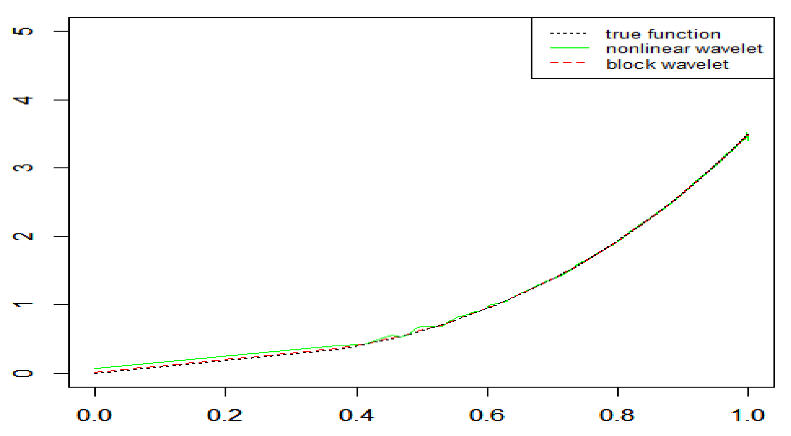
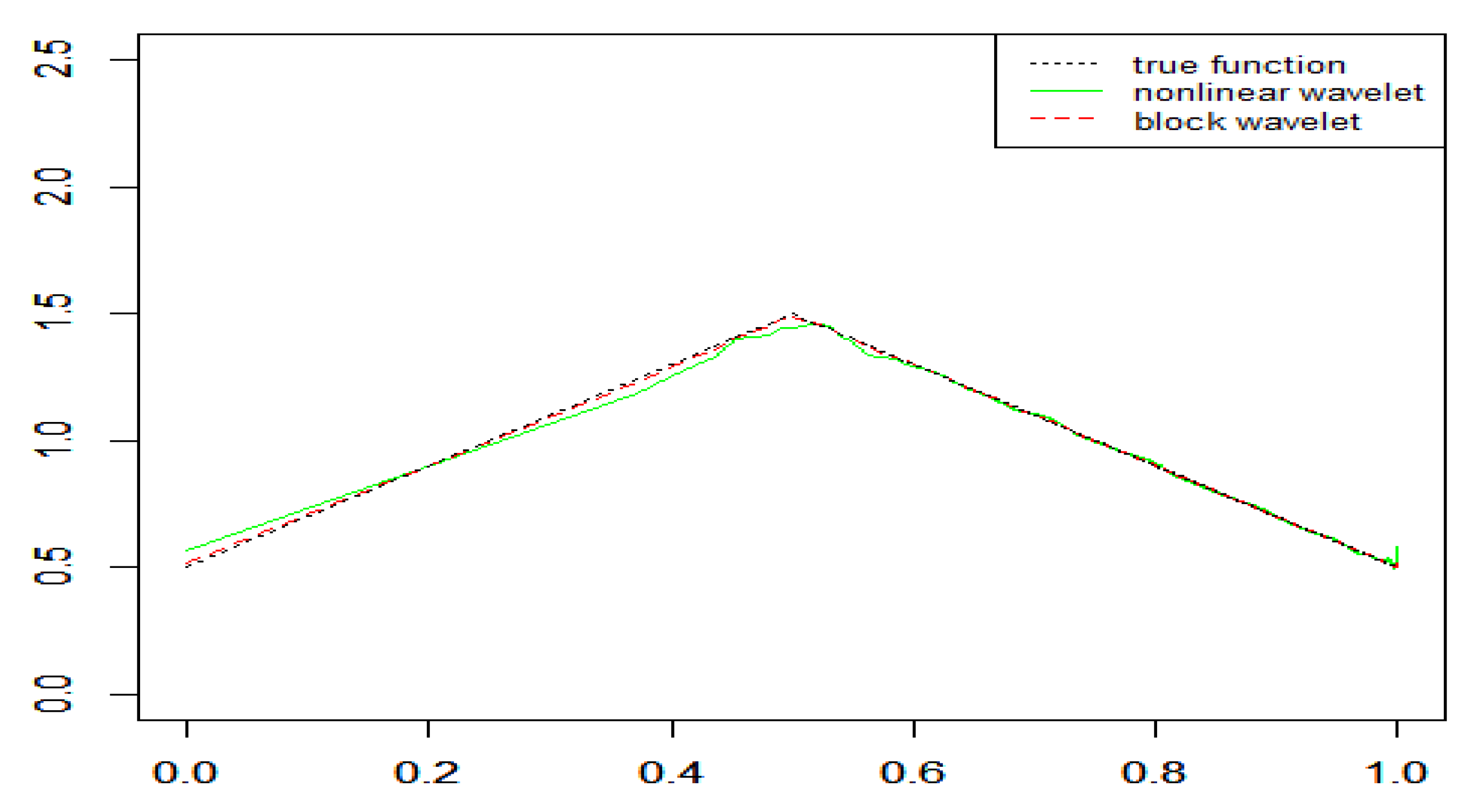
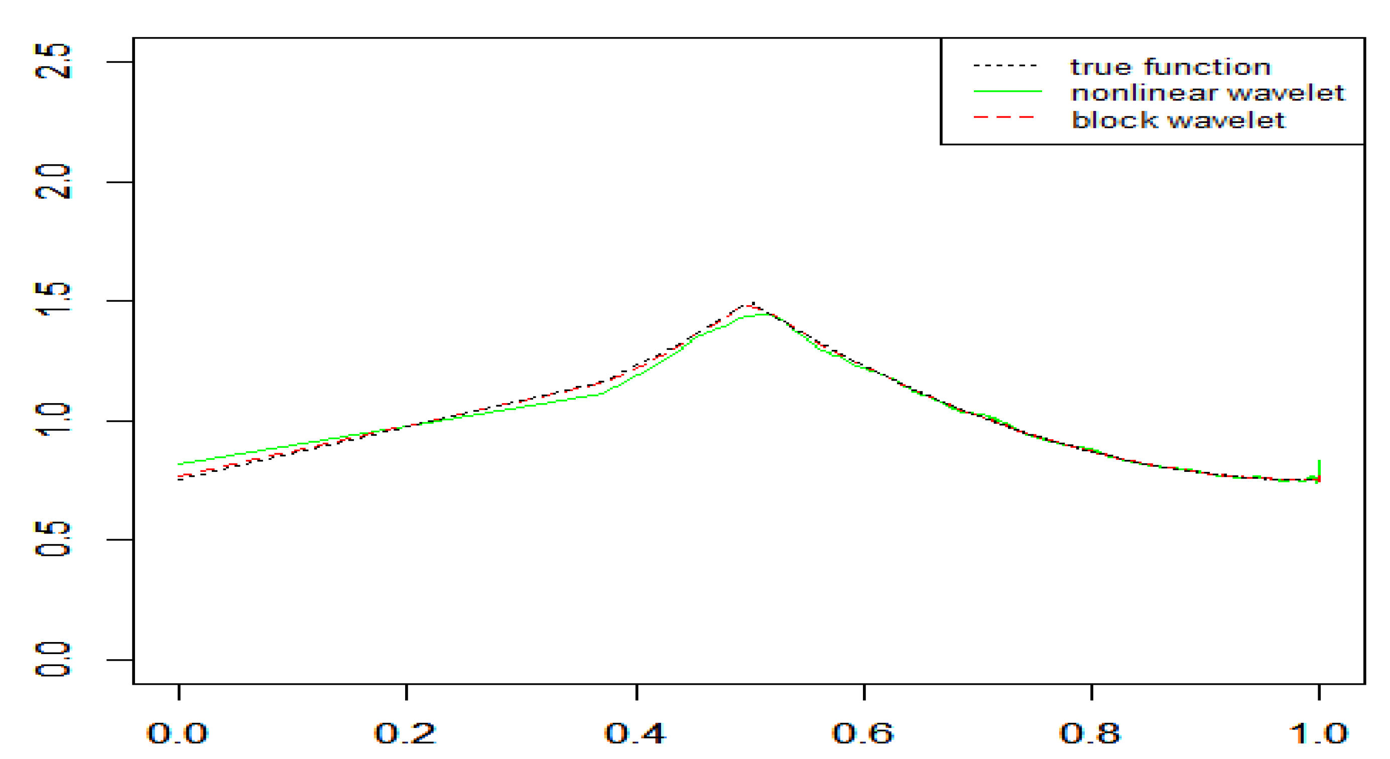
Let $L={\left(logn\right)}^{\left(p\vee 2\right)}$ and divide the set $\left\{0,1,\cdots ,2^{i-1}\right\}$ into consecutive, non-overlapping blocks of length L at every resolution level i, i.e.,

$${\Delta }_{im}=\left\{j:\left(m-1\right)L+1\le j\le mL\right\},m\in \mathbb{Z}.$$

Consider ${\widehat{\mu }}_n={\left(\frac{1}{n}{\displaystyle \sum _{t=1}^n}\frac{1}{\eta \left(Y_t\right)}\right)}^{-1}$ as the estimator of $\mu$. Define ${\widehat{\alpha }}_{i_{0}j}=\frac{{\widehat{\mu }}_n}{n}{\displaystyle \sum _{t=1}^n}\frac{1}{\eta \left(Y_t\right)}{\psi }_{i_{0}j}\left(Y_t\right)$ and ${\widehat{\beta }}_{ij}=\frac{{\widehat{\mu }}_n}{n}{\displaystyle \sum _{t=1}^n}\frac{1}{\eta \left(Y_t\right)}{\psi }_{ij}\left(Y_t\right)$. Denote $i_0=\frac{p\vee 2}{2}{log}_2\left({log}_{2}n\right)$ and $i_1={log}_2\left(n/{log}_{2}n\right)$ and let ${\displaystyle \sum _{\left(im\right)}}$ represent the summation over $j\in {\Delta }_{im}$. Then, the block thresholding estimator is given by:

$$\widehat{g}\left(y\right)=\sum _{j=0}^{2^{i_0}-1}{\widehat{\alpha }}_{i_{0}j}{\phi }_{i_{0}j}\left(y\right)+\sum _{i=i_0}^{i_1-1}\sum _m^{}\sum _{\left(im\right)}\left({\widehat{\beta }}_{ij}{\psi }_{ij}\left(y\right)\right)I\left({\widehat{B}}_{im}>\lambda \right),$$

(5)

where ${\widehat{B}}_{im}={\left(L^{-1}{\displaystyle \sum _{\left(im\right)}}{\left|{\widehat{\beta }}_{ij}^{}\right|}^p\right)}^{1/p}$ and the threshold is set to $\lambda =\sqrt{48{\left(c_2^{-1}\mu +c_1\right)}^2{n}^{-1}}$.

We outline the pointwise convergence rate of the wavelet density estimator $\widehat{g}\left(y\right)$ in the following theorem.

Theorem 1. 

Let $Y_1,Y_2,\cdots ,Y_n$ be an identically distributed NA sequence in Model (1). Suppose $g\in B_{h,q}^s$ and $s>max\left\{1/h,1/2\right\}$. For the block thresholding wavelet estimator $\widehat{g}\left(y\right)$ defined by (5), if the conditions (A1) and (A2) are satisfied, then for $1\le p<\infty$ and $h\ge p/\left(2s+1\right)$, a positive constant C exists, such that:

$$\underset{g\in B_{h,q}^s}{sup}E\int {\left(\widehat{g}\left(y\right)-g\left(y\right)\right)}^{2}dy\le \left\{\begin{array}{c}C{n}^{-ps/\left(2s+1\right)},\begin{array}{cc}\begin{array}{cc}& \end{array}& \begin{array}{cc}& \begin{array}{ccc}& & \begin{array}{cc}for& h\ge p,\end{array}\end{array}\end{array}\end{array}\\ C{n}^{-ps/\left(2s+1\right)}{\left(logn\right)}^{ps/\left(2s+1\right)},\begin{array}{cc}& \begin{array}{cc}for& p/\left(2s+1\right)\le h<p.\end{array}\end{array}\end{array}\right.$$

Remark 2. 

The block thresholding wavelet estimator is adaptive since $i_{0}and{i}_1$ do not rely on $s,h,q$. If $p=2$ and $\eta \left(y\right)\equiv 1$, Model (1) reduces to the standard density estimation model and the convergence rate in Theorem 1 is the same as the results of Cai and Chicken [16]. If the NA bias reduces to the independent bias, the results of the Theorem 1 become Theorem (4.1) in Chesneau [3].

Remark 3. 

With the presence of NA bias, Liu and Xu [14] and Guo and Kou [15] established the near optimal convergence rates (up to a logarithmic term) of a nonlinear wavelet estimator for the density function in Model (1). Note that the logarithmic term in the convergence rate has been removed in Theorem 1, which improves the convergence rates in [14,15].

4. Simulation Study

We used the method in Alam and Saxena [5] and Liu and Xu [14] to generate NA samples, firstly drawing n samples $Z_1,Z_2,\cdots ,Z_n$ from the distribution $Beta\left(2,2n-2\right)$, then choosing $Y_t=Z_t^{\delta }$( $\delta >0$). Thus, $Y_1,Y_2,\cdots ,Y_n$ are NA (refer to Liu and Xu [14]). Throughout the simulations, we took $\delta =\frac{1}{7}$.

Now, we provide three examples including the linear and nonlinear density functions, and their derivatives are continuous and discontinuous.

Example 1. 

Let $\eta \left(y\right)=y$ and $g\left(y\right)=3y^3+\frac{y}{2},y\in \left[0,1\right]$, then $g\left(y\right)$ is nonlinear density function and its derivative is continuous, $\mu =\frac{23}{30}$ and:

$$f\left(y\right)=\frac{30}{23}\left(3y^4+\frac{y^2}{2}\right),0\le y\le 1.$$

Example 2. 

Let $\eta \left(y\right)=y+1$ and:

$$g\left(y\right)=\left\{\begin{array}{c}2y+\frac{1}{2},\begin{array}{cc}& 0\le y\le \frac{1}{2},\end{array}\\ -2y+\frac{5}{2},\begin{array}{cc}& \frac{1}{2}<y\le 1.\end{array}\end{array}\right.$$

$g\left(y\right)$ is a linear continuous function but its derivative is discontinuous at $y=\frac{1}{2}$. We have $\mu =\frac{13}{12}$ and:

$$f\left(y\right)=\left\{\begin{array}{c}\frac{12}{13}\left(2y^2+\frac{5}{2}y+\frac{1}{2}\right),\begin{array}{cc}& 0\le y\le \frac{1}{2},\end{array}\\ \frac{12}{13}\left(-2y^2+\frac{1}{2}y+\frac{5}{2}\right),\begin{array}{cc}& \frac{1}{2}<y\le 1.\end{array}\end{array}\right.$$

Example 3. 

Let $\eta \left(y\right)=y+1$ and

$$g\left(y\right)=\left\{\begin{array}{c}3y^2+\frac{3}{4},\begin{array}{cc}& 0\le y\le \frac{1}{2},\end{array}\\ 3y^2-6y+\frac{15}{4},\begin{array}{cc}& \frac{1}{2}<y\le 1.\end{array}\end{array}\right.$$

$g\left(y\right)$ is a nonlinear continuous function but its derivative is discontinuous at $y=\frac{1}{2}$. We have $\mu =\frac{3}{2}$ and:

$$f\left(y\right)=\left\{\begin{array}{c}\frac{2}{3}\left(3y^3+3y^2+\frac{3}{4}y+\frac{3}{4}\right),\begin{array}{cc}& 0\le y\le \frac{1}{2},\end{array}\\ \frac{2}{3}\left(3y^3-3y^2-\frac{9}{4}y+\frac{15}{4}\right),\begin{array}{cc}& \frac{1}{2}<y\le 1.\end{array}\end{array}\right.$$

For the block wavelet threshold, we set $c_2=\mu$ and $c_1=\underset{1\le t\le n}{max}\left\{g\left(Y_t\right)\right\}+1$. To evaluate the performance of the density estimators, we considered the MSE, which is defined as:

$$\mathrm{MSE}=\frac{1}{n}\sum _{t=1}^n{\left(g^{est}\left(Y_t\right)-g\left(Y_t\right)\right)}^2.$$

Figure 1, Figure 2 and Figure 3 display the recovery of the density functions by wavelet density estimators for NA samples in the above examples.

Table 1. The MSEs of the block and nonlinear wavelet estimators.

n	Example 1		Example 2		Example 3
	Block	Nonlinear	Block	Nonlinear	Block	Nonlinear
512	0.0047	0.0072	0.0064	0.0102	0.0067	0.0114
1024	0.0043	0.0065	0.0056	0.0098	0.0054	0.0101
2048	0.0039	0.0058	0.0053	0.0096	0.0048	0.0093

lists the MSEs of these estimators. The results indicated both the nonlinear wavelet method and the block thresholding wavelet method performed well in the density estimation problem even though the samples were NA size-biased. The block wavelet density estimator performed better than the nonlinear wavelet density estimator in terms of the MSE; the estimations were increasingly accurate with increasing sample size.

5. Proof of Theorem 1

The proof of Theorem 1 is similar to that of Theorem (4.2) in Chesneau [20] and Theorem (4.1) in Chesneau [3]. The difference is that we considered that the samples were not only biased, but also NA. Hence, we had to overcome some non-trivial technical difficulties. Before elaborating the detailed proof, we introduce some basic properties and inequalities of the NA sequence in the following lemmas.

Lemma 1. 

[13]. For a sequence of NA random variables $Z_1,Z_2,cdots,Z_n$ and the non-empty subsets $B_1,B_2,\cdots ,B_k$ of $\left\{1,2,\cdots ,n\right\}$, if $B_1,B_2,\cdots ,B_k$ are pairwise disjoint and $f_1,f_2,\cdots ,f_k$ are k coordinate-wise non-decreasing Borel functions, then $f_1(Z_t,t\in B_1),f_2(Z_t,t\in B_2),\cdots ,f_k(Z_t,t\in B_k)$ are still NA.

Lemma 2. 

[20]. Let $\left\{Z_t,t\ge 1\right\}$ be NA random variables and $\left\{Z_t^{*},t\ge 1\right\}$ be independent random variables with the same marginal distribution as $Z_t^{}$. If f is a non-decreasing function, then:

$$E\left[f\left(\underset{1\le k\le n}{max}\left|\sum _{t=1}^k{Z}_t\right|\right)\right]\le E\left[f\left(\underset{1\le k\le n}{max}\left|\sum _{t=1}^k{Z}_t^{*}\right|\right)\right].$$

Lemma 3. 

[20]. If $\left\{Z_{t}andt\ge 1\right\}$ are NA random variables with $E{Z}_t=0$ and $E{\left|Z_t\right|}^2<\infty$, then we have:

(1) 

Rosenthal-type inequality: If $E{\left|Z_t\right|}^p<\infty$ for some $p\ge 2,$ then a constant $C_p$ (only depends on p) exists, such that:

$$E\left(\underset{1\le k\le n}{max}{\left|\sum _{t=1}^k{Z}_t\right|}^p\right)\le C_p\left\{\sum _{t=1}^{n}E{\left|Z_t\right|}^p+{\left(\sum _{t=1}^{n}E{Z}_t^2\right)}^{p/2}\right\}.$$

(2) 

Kolmogorov-type inequality: Denote $b_n^2={\displaystyle \sum _{t=1}^n}E{Z}_t^2$, we have, for all $0<b<1$, $z>0$ and $\tau >0$:

$$P\left(\underset{1\le k\le n}{max}\left|\sum _{t=1}^k{Z}_t\right|\ge z\right)\le 2P\left(\underset{1\le k\le n}{max}\left|Z_k^{}\right|>z\right)+\frac{1}{1-b}exp\left\{-\frac{{\tau }^{2}b}{2\left(\tau z+b_n^2\right)}\right\}.$$

Proof of Theorem 1. 

According to the proof of Theorem (4.1) in Chesneau [3], the proof of Theorem 1 will be completed if we can show that the moment inequality

$$E{\left|{\widehat{\beta }}_{ij}-{\beta }_{ij}\right|}^{2p}\le C{n}^{-p},$$

(6)

and the large deviation inequality

$$P\left({\left(\sum _{j\in {\Delta }_{im}}^{}{\left|{\widehat{\beta }}_{ij}-{\beta }_{ij}\right|}^p\right)}^{1/p}\ge \frac{\lambda }{2}{\left(logn\right)}^{-1/2}\right)\le n^{-p},$$

(7)

hold at resolution level i (the case of primary resolution level $i_0$ can be treated similarly). Therefore, the remainder of the proof is composed of the following two parts.

Part one: Moment inequality. By the proof of Proposition 4.1 in Chesneau [3], we have that the inequality (6) is equivalent to

$$E{\left|{\widehat{\beta }}_{ij}-{\beta }_{ij}\right|}^{2p}\le C_p\left(G_{ij}+H_{ij}\right),$$

(8)

where:

$$G_{ij}=E\left({\left|\mu n^{-1}\sum _{t=1}^n{\eta }^{-1}\left(Y_t\right){\psi }_{ij}-{\beta }_{ij}\right|}^{2p}\right),$$

$$H_{ij}=E\left({\left|n^{-1}\sum _{t=1}^n{\eta }^{-1}\left(Y_t\right)-{\mu }^{-1}\right|}^{2p}\right).$$

We first consider the term $G_{ij}$. Write:

$$n^{-1}\sum _{t=1}^n\mu {\eta }^{-1}\left(Y_t\right){\psi }_{ij}-{\beta }_{ij}=n^{-1}\sum _{t=1}^n\left(\mu {\eta }^{-1}\left(Y_t\right){\psi }_{ij}-{\beta }_{ij}\right)=:n^{-1}\sum _{t=1}^n{\xi }_t.$$

Since $\psi$ is a bounded variation function, then two bounded nonnegative nondecreasing functions exist, $\overline{\psi }$ and $\tilde{\psi }$, such that $\psi =\overline{\psi }-\tilde{\psi }$. Denote:

$${\overline{\xi }}_t=\mu {\eta }^{-1}\left(Y_t\right){\overline{\psi }}_{ij}\left(Y_t\right)-{\overline{\beta }}_{ij},{\tilde{\xi }}_t=\mu {\eta }^{-1}\left(Y_t\right){\tilde{\psi }}_{ij}\left(Y_t\right)-{\tilde{\beta }}_{ij},$$

(9)

where ${\overline{\beta }}_{ij}={\int }_0^{1}g\left(y\right){\overline{\psi }}_{ij}\left(y\right)dy$ and ${\tilde{\beta }}_{ij}={\int }_0^{1}g\left(y\right){\tilde{\psi }}_{ij}\left(y\right)dy$ and, hence, ${\xi }_t={\overline{\xi }}_t-{\tilde{\xi }}_t$. As Lemma 1 and $E\left({\xi }_1\right)={\int }_0^1\mu {\eta }^{-1}\left(y\right){\psi }_{ij}\left(y\right)\left(g\left(y\right)\eta \left(y\right){\mu }^{-1}\right)dy-{\beta }_{ij}=0$, ${\overline{\xi }}_t$ and ${\tilde{\xi }}_t$ ($t=1,2,\cdots ,n$) are zero NA random variables according to the monotonicity of $\eta \left(y\right)$ in assumption (A2).

Note that $\left|{\beta }_{ij}\right|\le {\left({\int }_0^1{g}^2\left(y\right)dy\right)}^{1/2}{\left({\int }_0^1{\psi }_{ij}^2\left(y\right)dy\right)}^{1/2}\le {\mathrm{c}}_1$ and $\left|{\psi }_{ij}\left(y\right)\right|\le \underset{y\in \left[0,1\right]}{sup}\left|{\psi }_{ij}\left(y\right)\right|\le 2^{j/2}\underset{y\in \left[0,1\right]}{sup}\left|\psi \left(y\right)\right|$ by assumption (A2) and Model (4). It follows that:

$$\begin{array}{ccc}E\left({\left|{\overline{\xi }}_1\right|}^p\right)\hfill & =\hfill & 2^{p-1}\left(E\left({\left|\mu {\eta }^{-1}\left(Y_1\right){\overline{\psi }}_{ij}\left(Y_1\right)\right|}^p\right)+{\left|{\overline{\beta }}_{ij}\right|}^p\right)\hfill \\ \hfill & \le \hfill & 2^{p-1}\left({\mu }^p{c}_2^{-\left(p-1\right)}{2}^{j\left(p-2\right)/2}{\left(\underset{y\in \left[0,1\right]}{sup}\left|\psi \left(y\right)\right|\right)}^{p-2}E\left({\eta }^{-1}\left(Y_1\right){\overline{\psi }}_{ij}^2\left(Y_1\right)\right)+c_1^p\right).\hfill \end{array}$$

For any $y\in \left[0,1\right]$, we have:

$$\begin{array}{cc} \hfill & E\left({\eta }^{-1}\left(Y_1\right){\overline{\psi }}_{ij}^2\left(Y_1\right)\right)\hfill \\ =\hfill & {\int }_0^1{\eta }^{-1}\left(y\right){\overline{\psi }}_{ij}^2\left(y\right)\left({\mu }^{-1}\eta \left(y\right)g\left(y\right)\right)dy\hfill \\ \le \hfill & {\mu }^{-1}{c}_1{\int }_0^1{\overline{\psi }}_{ij}^2\left(y\right)dy\le {\mu }^{-1}{c}_1.\hfill \end{array}$$

Hence, for all resolution levels $i_0\le i\le i_1$:

$$\begin{array}{ccc}E\left({\left|{\xi }_1\right|}^p\right)\hfill & \le \hfill & 2^{p-1}\left(c_1{\mu }^{p-1}{c}_2^{-\left(p-1\right)}{2}^{j\left(p-2\right)/2}{\left(\underset{y\in \left[0,1\right]}{sup}\left|\psi \left(y\right)\right|\right)}^{p-2}+c_1^p\right)\hfill \\ \hfill & \le \hfill & 2^{p-1}\left(C{n}^{\left(p-2\right)/2}+c_1^p\right)=O\left(n^{\left(p-2\right)/2}\right).\hfill \end{array}$$

Resorting to the Rosenthal-type inequality in Lemma 3, we obtain:

$$E\left({\left|n^{-1}\sum _{t=1}^n{\overline{\xi }}_t\right|}^{2p}\right)\le C\left(n^{1-2p}E\left({\xi }_1^{2p}\right)+n^{-p}{\left(E\left({\xi }_1^p\right)\right)}^p\right)=O\left(n^{-p}\right).$$

Similarly, for ${\tilde{\xi }}_t$, we have:

$$E\left({\left|n^{-1}\sum _{t=1}^n{\tilde{\xi }}_t\right|}^{2p}\right)=O\left(n^{-p}\right).$$

Recall that ${\xi }_t={\overline{\xi }}_t-{\tilde{\xi }}_t$, then we obtain:

$$G_{jk}=E\left({\left|n^{-1}\sum _{t=1}^n{\xi }_t\right|}^{2p}\right)\le \frac{1}{n^{2p}}\left(E{\left|\sum _{t=1}^n{\overline{\xi }}_t\right|}^{2p}+E{\left|\sum _{t=1}^n{\tilde{\xi }}_t\right|}^{2p}\right)=O\left(n^{-p}\right).$$

(10)

Now, we consider the term $H_{ij}$. Denote ${\zeta }_t=\frac{1}{\eta \left(Y_t\right)}-\frac{1}{\mu }$. It is easy to check that $E\left({\left|{\zeta }_1\right|}^p\right)\le 2^{p-1}\left(E\left({\eta }^{-p}\left(Y_1\right)\right)+{\mu }_{}^{-p}\right)\le c_1$. Resorting to the Rosenthal-type inequality again, we have:

$$\begin{array}{ccc}{H}_{ij}\hfill & =\hfill & E\left({\left|n^{-1}{\displaystyle \sum _{t=1}^n}{\zeta }_t\right|}^{2p}\right)\hfill \\ \hfill & \le \hfill & C\left(n^{1-2p}E\left({\zeta }_1^{2p}\right)+n^{-p}{\left(E\left({\zeta }_1^p\right)\right)}^p\right)\hfill \\ \hfill & \le \hfill & C\left(n^{1-2p}+n^{-p}\right)=O\left(n^{-p}\right).\hfill \end{array}$$

(11)

Consequently, the inequality (6) is followed by (8), (10), and (11).

Part two: Large deviation inequality. From the proof of Proposition 4.2 in Chesneau [3], we know that the inequality (7) is bounded by:

$$\begin{array}{cc} \hfill & P\left({\left({\displaystyle \sum _{j\in {\Delta }_{im}}^{}}{\left|{\widehat{\beta }}_{ij}-{\beta }_{ij}\right|}^p\right)}^{1/p}\ge \sqrt{32{\left(c_2^{-1}\mu +c_1\right)}^2}{n}^{-1/2}{\left({log}_{2}n\right)}^{1/2}\right)\hfill \\ \le \hfill & P\left(\left|\frac{1}{n}{\displaystyle \sum _{t=1}^n}\left(\frac{1}{\eta \left(Y_t\right)}-\frac{1}{\mu }\right)\right|\ge \sqrt{8{\left(c_2^{-1}\mu +c_1\right)}^2}{n}^{-1/2}{\left({log}_{2}n\right)}^{1/2}\right)\hfill \\ \hfill & +P\left({\left(n^{-1}{\displaystyle \sum _{j\in {\Delta }_{im}}^{}}{\left|\frac{{\widehat{\mu }}_n}{\eta \left(Y_t\right)}{\psi }_{ij}\left(Y_t\right)-{\beta }_{ij}\right|}^p\right)}^{1/p}\ge \sqrt{8{\left(c_2^{-1}\mu +c_1\right)}^2}{n}^{-1/2}{\left({log}_{2}n\right)}^{1/2}\right)\hfill \\ =:\hfill & S_1+S_2.\hfill \end{array}$$

Now, let us consider the upper bounds of $S_1$ and $S_2$, separately.

Bound for $S_1$: Recall that ${\zeta }_t=\frac{1}{\eta \left(Y_t\right)}-\frac{1}{\mu }$ and $t=1,\cdots ,n$, are NA random variables with zero mean and finite variance ${\sigma }_{}^2$. Hence, the triangular inequality yields:

$$\left|{\zeta }_t\right|\le {\mu }^{-1}+{\eta }^{-1}\left(Y_t\right)\le 2c_2^{-1}.$$

Taking $\tau =n^{1/2}{\left({log}_{2}n\right)}^{1/2}$, $b=\frac{1}{2}$ and $z=2c_2^{-1}$, using the Kolmogorov-type inequality in Lemma 3, we have:

$$\begin{array}{ccc}{S}_1\hfill & \le \hfill & P\left(\underset{1\le t\le n}{max}\left|{\displaystyle \sum _{t=1}^n}{\zeta }_t\right|\ge C{n}^{1/2}{\left({log}_{2}n\right)}^{1/2}\right)\hfill \\ \hfill & \le \hfill & 4exp\left\{-\frac{8{\left(c_2^{-1}\mu +c_1\right)}^{2}n\left({log}_{2}n\right)}{4\left(2\sqrt{8{\left(c_2^{-1}\mu +c_1\right)}^2}{c}_2^{-1}{n}^{1/2}{\left({log}_{2}n\right)}^{1/2}+n{\sigma }^2\right)}\right\}\hfill \\ \hfill & \le \hfill & 4exp\left\{-\frac{C^2}{4{\sigma }^2}{log}_{2}n\right\}=O\left(n^{-p}\right).\hfill \end{array}$$

(12)

Bound for $S_2$: Recall that $L={\left({log}_{2}n\right)}^{\left(p\vee 2\right)}$, we set ${\lambda }_{*}=\sqrt{8{\left(c_2^{-1}\mu +c_1\right)}^2}{n}^{-1/2}{\left({log}_{2}n\right)}^{1/2}$, then $S_2\le O\left(n^{-p}\right)$ implies that:

$$P\left\{{\left(n^{-1}{\displaystyle \sum _{j\in {\Delta }_{im}}^{}}{\left|\frac{{\widehat{\mu }}_n}{\eta \left(Y_t\right)}{\psi }_{ij}\left(Y_t\right)-{\beta }_{ij}\right|}^p\right)}^{1/p}\ge {\lambda }_{*}\right\}\le Cexp\left\{-\frac{n{\lambda }_{*}^2}{8{\left(c_2^{-1}\mu +c_1\right)}^2}\right\}.$$

(13)

Now, we will check the inequality in (13). Let $d=\frac{p}{p-1}$ and define a set $\Theta =\left\{\theta =\left({\theta }_1,{\theta }_2,\cdots ,{\theta }_L\right)\in {\mathbb{R}}^L:{\displaystyle \sum _{t=1}^L}{\theta }_t^d\le 1\right\}$. By the elementary inequality and the argument of duality, we show that for all integers $i,m$:

$$\begin{array}{ccc}{\left({\displaystyle \sum _{j\in {\Delta }_{im}}^{}}{\left|n^{-1}{\displaystyle \sum _{t=1}^n}\frac{\mu }{\eta \left(Y_t\right)}{\psi }_{ij}\left(Y_t\right)-{\beta }_{ij}\right|}^p\right)}^{1/p}\hfill & \le \hfill & {\left({\displaystyle \sum _{j\in {\Delta }_{im}}^{}}{\left|n^{-1}{\displaystyle \sum _{t=1}^n}\frac{\mu }{\eta \left(Y_t\right)}{\psi }_{ij}\left(Y_t\right)-{\beta }_{ij}\right|}^2\right)}^{1/2}\hfill \\ \hfill & =\hfill & \underset{\theta \in \Theta }{sup}{\displaystyle \sum _{j=1}^L}{\theta }_j^{}\left(n^{-1}{\displaystyle \sum _{t=1}^n}\frac{\mu }{\eta \left(Y_t\right)}{\psi }_{ij}\left(Y_t\right)-{\beta }_{ij}\right).\hfill \end{array}$$

(14)

Therefore, substituting Equation (14) into Equation (13) produces:

$$P\left\{\underset{\theta \in \Theta }{sup}{\displaystyle \sum _{j=1}^L}{\theta }_j^{}\left(n^{-1}{\displaystyle \sum _{t=1}^n}\frac{\mu }{\eta \left(Y_t\right)}{\psi }_{ij}\left(Y_t\right)-{\beta }_{ij}\right)\ge {\lambda }_{*}^{}\right\}\le Cexp\left(-\frac{n{\lambda }_{*}^2}{8{\left(c_2^{-1}\mu +c_1\right)}^2}\right).$$

(15)

To prove Equation (15), we define a stochastic process $\left\{T_n\left(\theta \right),\theta \in \Theta \right\}$ with

$$T_n\left(\theta \right)={\displaystyle \sum _{j=1}^L}{\theta }_j^{}\left(n^{-1}{\displaystyle \sum _{t=1}^n}\frac{\mu }{\eta \left(Y_t\right)}{\psi }_{ij}\left(Y_t\right)-{\beta }_{ij}\right).$$

Note that ${\beta }_{ij}={\int }_0^{1}g\left(y\right){\psi }_{ij}\left(y\right)dy=\frac{1}{n}{\displaystyle \sum _{t=1}^n}g\left(Y_t\right){\psi }_{ij}\left(Y_t\right)$. Denote $e_t=\frac{\mu }{\eta \left(Y_t\right)}-g\left(Y_t\right)$, then $T_n\left(\theta \right)$ can be rewritten as:

$$T_n\left(\theta \right)=\frac{1}{n}{\displaystyle \sum _{t=1}^n}{e}_t{\displaystyle \sum _{j=1}^L}{\theta }_j^{}{\psi }_{ij}\left(Y_t\right).$$

Similar to the definition of $\overline{\psi }$ and $\tilde{\psi }$ in Equation (9), we set ${\overline{T}}_n\left(\theta \right)=\frac{1}{n}{\displaystyle \sum _{t=1}^n}{e}_t{\displaystyle \sum _{j=1}^L}{\theta }_j^{}{\overline{\psi }}_{ij}\left(Y_t\right)$, ${\tilde{T}}_n\left(\theta \right)=\frac{1}{n}{\displaystyle \sum _{t=1}^n}{e}_t{\displaystyle \sum _{j=1}^L}{\theta }_j^{}{\tilde{\psi }}_{ij}\left(Y_t\right)$. Let $\epsilon >0$, if $\left|\epsilon {\overline{T}}_n^{}\left(\theta \right)\right|\le 1$, then:

$$\begin{array}{ccc}E\underset{\theta \in \Theta }{sup}exp\left\{\epsilon \left|{\overline{T}}_n^{}\left(\theta \right)\right|\right\}\hfill & \le \hfill & 1+{\displaystyle \sum _{k=2}^{\infty }}\frac{E\underset{\theta \in \Theta }{sup}{\left(\left|\epsilon {\overline{T}}_n\left(\theta \right)\right|\right)}^k}{k!}\hfill \\ \hfill & \le \hfill & 1+{\epsilon }^{2}E\underset{\theta \in \Theta }{sup}{\left|{\overline{T}}_n^{}\left(\theta \right)\right|}^2\left\{\frac{1}{2!}+\frac{1}{3!}+\cdots \right\}\hfill \\ \hfill & \le \hfill & exp\left\{{\epsilon }^{2}E\underset{\theta \in \Theta }{sup}{\left|{\overline{T}}_n^{}\left(\theta \right)\right|}^2\right\}.\hfill \end{array}$$

(16)

Recall that ${\displaystyle \sum _{j=1}^L}{\theta }_j^d\le 1$ and $\frac{1}{d}+\frac{1}{p}=1$, $\left|e_t\right|\le \left|\frac{\mu }{\eta \left(Y_t\right)}\right|+\left|g\left(Y_t\right)\right|\le c_2^{-1}\mu +c_1$, invoking the Hölder’s inequality produces:

$$\begin{array}{ccc}exp\left\{E\underset{\theta \in \Theta }{sup}{\left|\epsilon {\overline{T}}_n^{}\left(\theta \right)\right|}^2\right\}\hfill & \le \hfill & \underset{\theta \in \Theta }{sup}{\displaystyle \prod _{t=1}^n}\left(exp\left\{E\frac{{\epsilon }^2}{n^2}{\displaystyle \sum _{j=1}^L}{\left|{\theta }_j^{}{\overline{\psi }}_{ij}\left(Y_t\right)\right|}^2{\left(e_t^{}\right)}^2\right\}\right)\hfill \\ \hfill & \le \hfill & \underset{\theta \in \Theta }{sup}{\displaystyle \prod _{t=1}^n}\left(exp\left\{\frac{{\left(c_2^{-1}\mu +c_1\right)}^2{\epsilon }^2}{n^2}{\left({\displaystyle \sum _{j=1}^L}{\theta }_j^d\right)}^{2/d}{\left({\displaystyle \sum _{j=1}^L}{\overline{\psi }}_{ij}^p\left(Y_t\right)\right)}^{2/p}\right\}\right)\hfill \\ \hfill & \le \hfill & exp\left\{\frac{{\left(c_2^{-1}\mu +c_1\right)}^2{\epsilon }^2}{n^2}{\displaystyle \sum _{t=1}^n}{\left({\displaystyle \sum _{j=1}^L}{\overline{\psi }}_{ij}^p\left(Y_t\right)\right)}^{2/p}\right\}.\hfill \end{array}$$

Note that when $t=j$, ${\left|{\overline{\psi }}_{ij}\left(Y_t\right)\right|}^p=1,$ and for all $t\ne j$, ${\left|{\overline{\psi }}_{ij}\left(Y_t\right)\right|}^p=0$. Hence, for every $j\left(j=1,2,\cdots ,L\right)$, only a counterpart $t=j$ exists, such that ${\left|{\psi }_{ij}\left(Y_t\right)\right|}^p=1$; that is, ${\displaystyle \sum _{t=1}^n}{\left({\displaystyle \sum _{j=1}^L}{\left|{\psi }_{ij}\left(Y_t\right)\right|}^p\right)}^{2/p}=L^{2/p},$ which leads to:

$$exp\left\{{\epsilon }^{2}E\underset{\theta \in \Theta }{sup}{\left|{\overline{T}}_n^{}\left(\theta \right)\right|}^2\right\}\le Cexp\left\{\frac{{\left(c_2^{-1}\mu +c_1\right)}^2{\epsilon }^2{L}^{2/p}}{n^2}\right\}.$$

(17)

Now we consider the case $\left|\epsilon {\overline{T}}_n^{}\left(\theta \right)\right|>1$. By Lemmas 1 and 2, for $\epsilon >0$, we obtain:

$$\begin{array}{ccc}E\underset{\theta \in \Theta }{sup}exp\left\{\left|\epsilon {\overline{T}}_n^{}\left(\theta \right)\right|\right\}\hfill & \le \hfill & Eexp\left\{E\underset{\theta \in \Theta }{sup}{\left|\epsilon {\overline{T}}_n^{}\left(\theta \right)\right|}^2\right\}\hfill \\ \hfill & \le \hfill & \underset{\theta \in \Theta }{sup}{\displaystyle \prod _{t=1}^n}E\left(exp\left\{\frac{{\epsilon }^2}{n^2}{\displaystyle \sum _{j=1}^L}{\left|{\theta }_j^{}{\overline{\psi }}_{ij}\left(Y_t\right)\right|}^2{\left(e_t^{}\right)}^2\right\}\right)\hfill \\ \hfill & \le \hfill & Cexp\left\{\frac{{\left(c_2^{-1}\mu +c_1\right)}^2{\epsilon }^2}{n^2}{\displaystyle \sum _{t=1}^n}{\left({\displaystyle \sum _{j=1}^L}{\left|{\psi }_{ij}\left(Y_t\right)\right|}^p\right)}^{2/p}\right\}\hfill \\ \hfill & \le \hfill & Cexp\left\{\frac{{\left(c_2^{-1}\mu +c_1\right)}^2{\epsilon }^2}{n}\right\}.\hfill \end{array}$$

(18)

Thus, using Equations (16)–(18) together, we derive that:

$$E\underset{\theta \in \Theta }{sup}exp\left\{\left|\epsilon {\overline{T}}_n^{}\left(\theta \right)\right|\right\}\le Cexp\left\{\frac{{\left(c_2^{-1}\mu +c_1\right)}^2{\epsilon }^2}{n}\right\}.$$

Likewise, for the term ${\tilde{T}}_n^{}\left(\theta \right)$:

$$E\underset{\theta \in \Theta }{sup}exp\left\{\left|\epsilon {\tilde{T}}_n^{}\left(\theta \right)\right|\right\}\le Cexp\left\{\frac{{\left(c_2^{-1}\mu +c_1\right)}^2{\epsilon }^2}{n}\right\}.$$

Applying Markov’s inequality, all ${\lambda }_{*}>0$ and $\epsilon >0$, we have:

$$P\left\{\underset{\theta \in \Theta }{sup}\left|{\overline{T}}_n^{}\left(\theta \right)\right|\ge {\lambda }_{*}\right\}\le \frac{Eexp\left\{\underset{\theta \in \Theta }{sup}{\overline{T}}_n^{}\left(\theta \right)\right\}}{exp\left\{\epsilon {\lambda }_{*}\right\}}\le exp\left\{-\epsilon {\lambda }_{*}+{\left(c_2^{-1}\mu +c_1\right)}^2{\epsilon }^2/n\right\},$$

(19)

$$P\left\{\underset{\theta \in \Theta }{sup}\left|{\tilde{T}}_n^{}\left(\theta \right)\right|\ge {\lambda }_{*}\right\}\le \frac{Eexp\left\{\underset{\theta \in \Theta }{sup}{\tilde{T}}_n^{}\left(\theta \right)\right\}}{exp\left\{\epsilon {\lambda }_{*}\right\}}\le exp\left\{-\epsilon {\lambda }_{*}+{\left(c_2^{-1}\mu +c_1\right)}^2{\epsilon }^2/n\right\}.$$

(20)

Taking $\epsilon =\frac{n{\lambda }_{*}}{2{\left(c_2^{-1}\mu +c_1\right)}^2}$ in Equations (19) and (20), we obtain:

$$P\left\{\underset{\theta \in \Theta }{sup}\left|{\overline{T}}_n^{}\left(\theta \right)\right|\ge {\lambda }_{*}\right\}\le Cexp\left\{-{\lambda }_{*}^{2}n/4{\left(c_2^{-1}\mu +c_1\right)}^2\right\},$$

$$P\left\{\underset{\theta \in \Theta }{sup}\left|{\tilde{T}}_n^{}\left(\theta \right)\right|\ge {\lambda }_{*}\right\}\le Cexp\left\{-{\lambda }_{*}^{2}n/4{\left(c_2^{-1}\mu +c_1\right)}^2\right\}.$$

Note that $\underset{\theta \in \Theta }{sup}{T}_n^{}\left(\theta \right)\le \underset{\theta \in \Theta }{sup}\left|{\overline{T}}_n^{}\left(\theta \right)-{\tilde{T}}_n^{}\left(\theta \right)\right|\le \underset{\theta \in \Theta }{sup}\left|{\overline{T}}_n^{}\left(\theta \right)\right|+\underset{\theta \in \Theta }{sup}\left|{\tilde{T}}_n^{}\left(\theta \right)\right|$; hence:

$$\begin{array}{ccc}P\left\{\underset{\theta \in \Theta }{sup}{T}_n^{}\left(\theta \right)\ge {\lambda }_{*}\right\}\hfill & \le \hfill & P\left\{\underset{\theta \in \Theta }{sup}\left|{\overline{T}}_n^{}\left(\theta \right)\right|\ge {\lambda }_{*}/2\right\}+P\left\{\underset{\theta \in \Theta }{sup}\left|{\tilde{T}}_n^{}\left(\theta \right)\right|\ge {\lambda }_{*}/2\right\}\hfill \\ \hfill & \le \hfill & Cexp\left\{-{\lambda }_{*}^{2}n/8{\left(c_2^{-1}\mu +c_1\right)}^2\right\}.\hfill \end{array}$$

This is the result of Equation (15) and thus concludes the proof of Theorem 1. □

References

1. Efromovich, S. Density estimation for biased data. Ann. Statist. 2004, 32, 1137–1161. [Google Scholar] [CrossRef] [Green Version]
2. Ramirez, P.; Vidakovic, B. Wavelet density estimation for stratified size-biased sample. J. Stat. Plan. Inference 2010, 140, 419–432. [Google Scholar] [CrossRef]
3. Chesneau, C. Wavelet block thresholding for density estimation in the presence of bias. J. Korean Stat. Soc. 2010, 39, 43–53. [Google Scholar] [CrossRef] [Green Version]
4. Guo, H.; Kou, J. Pointwise density estimation for biased sample. J. Comput. Appl. Math. 2019, 361, 444–458. [Google Scholar] [CrossRef]
5. Alam, K.; Saxena, K.L. Positive dependence in multivariate distributions. Commun. Stat. Theory Method. 1981, 10, 1183–1196. [Google Scholar]
6. Joag-Dev, K.; Proschan, F. Negative association of random variables with applications. Ann. Stat. 1983, 11, 286–295. [Google Scholar] [CrossRef]
7. Liang, H.Y. Complete convergence for weighted sums of negatively associated random variables. Statist. Probab. Lett. 2000, 48, 317–325. [Google Scholar] [CrossRef]
8. Matula, P. A note on the almost sure convergence of sums of negatively dependent random variables. Statist. Probab. Lett. 1992, 5, 209–212. [Google Scholar] [CrossRef]
9. Roussas, G.G. Asymptotic normality of random fields of positively or negatively associated processes. J. Multivariate Anal. 1994, 50, 152–173. [Google Scholar] [CrossRef] [Green Version]
10. Chen, P.; Sung, S.H. On the strong convergence for weighted sums of negatively associated random variables. Statist. Probab. Lett. 2014, 92, 45–52. [Google Scholar] [CrossRef]
11. Miao, Y.; Xu, W.; Chen, S. Some limit theorems for negatively associated random variables. Pro. Math. Sci. 2014, 124, 447–456. [Google Scholar] [CrossRef]
12. Wu, Y. On complete moment convergence for arrays of rowwise negatively associated random variables. RACSAM 2014, 108, 669–681. [Google Scholar] [CrossRef]
13. Chesneau, C.; Dewan, I.; Doosti, H. Wavelet linear density estimation for associated stratified size-biased sample. J. Nonparametr. Stat. 2012, 2, 429–445. [Google Scholar] [CrossRef]
14. Liu, Y.M.; Xu, J.L. Wavelet density estimation for negatively associated stratified size-biased sample. J. Nonparametr. Stat. 2014, 26, 537–554. [Google Scholar] [CrossRef]
15. Guo, H.J.; Kou, J.K. Pointwise density estimation based on negatively associated data. J. Inequal. Appl. 2019, 206, 1–16. [Google Scholar] [CrossRef]
16. Cai, T.; Chicken, E. Block thresholding for density estimation: Local and global adaptivity. J. Multivariate Anal. 2005, 95, 76–106. [Google Scholar]
17. Brown, L.; Cai, T.; Zhang, R.; Zhao, L. The root-unroot algorithm for density estimation as implemented via wavelet block thresholding. Probab. Theory Related Fields 2010, 146, 401–433. [Google Scholar] [CrossRef] [Green Version]
18. Chesneau, C. Wavelet estimation via block thresholding: A minimax study under the Lp risk. Statist. Sinica. 2008, 18, 1007–1024. [Google Scholar]
19. Donoho, D.L.; Johnstone, I.M. Minimax estimation via wavelet shrinkage. Ann. Stat. 1998, 26, 879–921. [Google Scholar] [CrossRef]
20. Shao, Q.M. A comparison theorem on maximum inequalities between negatively associated and independent random variables. J. Theoret. Probab. 2000, 13, 343–356. [Google Scholar] [CrossRef]
Figure 1. Recovery of the density function for NA samples in Example 1 ( n = 2048 ).
Mathematics 08 00176 g001
Figure 2. Recovery of the density function for NA samples in Example 2 ( n = 2048 ).
Mathematics 08 00176 g002
Figure 3. Recovery of the density function for NA samples in the Example 3 ( n = 2048 ).
Mathematics 08 00176 g003