Abstract
Extracellular matrix (ECM) proteins play an important role in a series of biological processes of cells. The study of ECM proteins is helpful to further comprehend their biological functions. We propose ECMP-RF (extracellular matrix proteins prediction by random forest) to predict ECM proteins. Firstly, the features of the protein sequence are extracted by combining encoding based on grouped weight, pseudo amino-acid composition, pseudo position-specific scoring matrix, a local descriptor, and an autocorrelation descriptor. Secondly, the synthetic minority oversampling technique (SMOTE) algorithm is employed to process the class imbalance data, and the elastic net (EN) is used to reduce the dimension of the feature vectors. Finally, the random forest (RF) classifier is used to predict the ECM proteins. Leave-one-out cross-validation shows that the balanced accuracy of the training and testing datasets is 97.3% and 97.9%, respectively. Compared with other state-of-the-art methods, ECMP-RF is significantly better than other predictors.
1. Introduction
The extracellular matrix is a macromolecule synthesized by animal cells that is distributed on the cell surface or between cells [1,2]. The ECM not only provides structural support to cells within the tumor but also provides anchorage and tissue separation for the cells. It also has a coherence effect to mediate communication between cells, and it contributes to survival and differentiation signals [3,4]. ECM proteins actively promote essential cellular processes such as differentiation, proliferation, adhesion, migration, and apoptosis [5,6,7,8]. ECM proteins in certain parts of etiology are the drivers of disease [9]. Defects of ECM proteins are associated with many human diseases (such as cancer, atherosclerosis, asthma, fibrosis, and arthritis), and modified ECM proteins help to understand complex pathologies [10,11]. ECM protein research contributes to the development of novel cell-adhesive biomaterials that are critical in many medical fields, such as cell therapy or tissue engineering [12,13]. The diversity of ECM proteins contributes to the diversity of ECM function; thus, they play a comprehensive biological role in the basic life activities of cells. Therefore, accurate recognition of ECM proteins plays a crucial role in physiology and pathology research.
ECM protein prediction is an important branch in the field of protein function research. Compared with time-consuming and laborious experimental methods, bioinformatics methods can integrate advanced machine learning methods to accurately and efficiently predict proteins by fusing sequence information, physicochemical properties, structural information, and evolutionary information. The construction of protein prediction models mainly focuses on three aspects. (1) Feature extraction of protein sequences. The amino-acid letter sequence is converted into a numerical sequence by a feature extraction method. At present, protein sequence feature extraction methods are mainly based on sequence information, physicochemical properties, evolutionary information, and structural information. (2) Feature selection. Eliminating redundant features by feature selection technology can not only reduce the dimension of the feature space but also improve the robustness of the prediction model. More importantly, in predictive models, feature selection can assess the importance of features and help discover the molecular mechanisms via which proteins perform their corresponding biological functions. (3) Model construction and model evaluation. A prediction algorithm is designed and a prediction model is built. An effective prediction algorithm can improve the generalization ability and prediction performance of the model. Because the machine learning method has the ability to train the model and prediction, it is widely used in proteomics. Current mainstream machine learning methods include random forest (RF) [14], naïve Bayes [15,16], decision tree (DT) [17], support vector machine (SVM) [18], extreme gradient boosting (XGBoost) [19], adaptive boosting (AdaBoost) [20], logistic regression (LR) [21], gradient boosting decision tree (GBDT) [22], etc.
Given the important research significance of ECM proteins in physiopathology, more and more researchers are committed to the prediction research of ECM proteins. Table 1 summarizes the prediction methods of ECM proteins.

Table 1.
The existing extracellular matrix (ECM) proteins prediction methods.
At present, a series of research results were obtained by predicting ECM proteins through bioinformatics and machine learning methods, but there is still room for improvement. Firstly, the development of an effective feature extraction method can achieve higher prediction accuracy. Extracting accurate feature vectors for proteins is a key step in successful prediction. Secondly, how to delete redundant information caused by feature fusion while retaining valid feature information is also one of the important directions of our research. The feature selection methods used in this paper include principal component analysis (PCA) [30], factor analysis (FA) [31], mutual information (MI) [32], least absolute shrinkage and selection operator (LASSO) [33], kernel principal component analysis (KPCA) [34], logistic regression (LR) [35], and elastic net (EN) [36,37]. Finally, how to choose prediction methods and tools with high calculation efficiency and good performance is also the focus of our research. Different from other methods, we explore a variety of sequence-based discriminant features, including sequence information, evolutionary information, and physicochemical properties. We use the synthetic minority oversampling technique (SMOTE) to deal with class imbalance between data. Instead of simply combining features that may cause information redundancy and unwanted noise, the optimal feature subset is selected by EN. We choose an RF classifier which hinders over-fitting in the prediction of ECM proteins.
In this paper, a new ECM proteins prediction method named ECMP-RF (extracellular matrix proteins prediction by random forest) is proposed. Firstly, we integrate encoding based on grouped weight (EBGW), pseudo amino-acid composition (PseAAC), pseudo position-specific scoring matrix (PsePSSM), a local descriptor (LD), and an autocorrelation descriptor (AD) to extract protein sequence features. Five kinds of feature coding information are fused as the initial feature space. Then, the SMOTE method is used to balance the samples. Thirdly, comparing seven different feature selection methods for prediction, the EN is used to select the feature vectors. Finally, the RF classifier is used to predict ECM proteins. Based on the prediction results, RF is selected as a classifier to construct a multi-feature fusion ECM protein prediction model. The balanced accuracy (BACC) obtained by leave-one-out cross-validation (LOOCV) on the training dataset and the testing dataset is as high as 97.28% and 97.94%, respectively. The prediction effect is higher than the currently known classification models. The source code and all datasets are available at https://github.com/QUST-AIBBDRC/ECMP-RF/.
2. Materials and Methods
2.1. Datasets
A dataset is mainly used for training and testing models. The quality of datasets has a direct effect on model construction. Therefore, establishing an ECM protein prediction model requires an objective and representative dataset. To compare with the existing research results, this paper uses a dataset constructed in the existing literature for experimental analysis, thereby ensuring the scientific relevance and fairness of the comparative analysis. Yang [27] took the dataset established by Kandaswamy [25] as the original training dataset and constructed a training dataset and testing dataset according to the principle of dataset construction. The training dataset and testing dataset contain 410 ECM proteins and 85 ECM proteins, respectively. At the same time, the training dataset and testing dataset contain 4464 non-ECM proteins and 130 non-ECM proteins, respectively.
2.2. Encoding Based on Grouped Weight
Zhang [38] proposed the encoding based on grouped weight (EBGW) method to extract the characteristics of the physicochemical properties of proteins. EBGW is widely used in research fields such as protein interactions [39,40], prediction of Golgi protein types [41], and prediction of protein mitochondrial localization [42]. EBGW is based on the physicochemical properties of amino-acid sequences. It uses the concept of “coarse graining” to convert protein sequences into binary characteristic sequences. The group weight coding of protein sequences is realized by introducing a regular weight function. Amino acids are the basic units of protein. The protein sequence is composed of 20 amino acids through a series of biochemical reactions. Different amino acids have different physicochemical properties. According to different physicochemical properties, amino acids can be divided into four categories. These are acidic amino acids , basic amino acids , neutral and polar amino acids , and neutral and hydrophobic amino acids . The above four types of amino acids can be combined one by one to obtain three new division methods: and , and , and . After a protein is mapped according to these three division methods, the protein sequence is reduced to a binary feature sequence.
The protein sequence is transformed into three binary sequences according to Equations (1)–(4).
where represents protein sequence characteristics. Given the sequence feature of length , weight refers to the number of occurrences of “” in the sequence, and rule weight refers to the frequency of occurrence. By dividing the raw sequence into subsequences, these features can be obtained. Then, the normal weight of each subsequence is calculated, thereby obtaining an -dimensional vector . The transformation from to is the group weight coding of sequence features. Thus, the three sequence features are used to obtain three vectors, and the three vectors are combined to obtain a -dimensional vector, denoted as , where is referred to as the group weight encoding of protein sequence .
2.3. Pseudo Amino-Acid Composition
Chou [43] proposed the pseudo amino-acid composition (PseAAC) to solve the problem of feature vector extraction in protein sequences. At present, PseAAC is widely used by researchers in proteomic fields, such as protein site prediction [44], protein structure prediction [41,45,46], protein subcellular localization prediction [47,48,49,50], and protein submitochondrion prediction [42,51]. The specific calculation steps of the PseAAC algorithm are shown in Equations (5) and (6).
where,
where represents the eigenvector, refers to the nearest correlation factor with a number of , and refers to the weight factor with a value of 0.05 [52]. represents the frequency of the -th amino acid in this sequence . In this method, the protein sequence is mapped to an ()-dimensional vector; the first 20 dimensions are the AAC, while the latter -dimensional is the sequence correlation factor, which can be obtained through the physicochemical properties of amino acids. The value cannot be greater than the shortest length of the protein sequence in the training set; thus, the value is between 10 and 50.
2.4. Pseudo Position-Specific Scoring Matrix
The pseudo position-specific scoring matrix (PsePSSM) was proposed by Chou and Shen. [53]. PsePSSM can not only extract sequence information, but also reflect sequence evolution information. It is extensively used in proteomics research. Qiu [54] predicted the location of protein mitochondria by integrating PsePSSM into general PseAAC. Shi [55] used PsePSSM to extract the features of a drug target. The method of PsePSSM is used to extract the features of a protein sequence. We use the multi-sequence homology matching tool position-specific iterated basic local alignment search tool (PSI-BLAST) to set the parameters to three iterations, and the PSSM of each protein sequence is shown in Equation (7).
The elements in a PSSM matrix are normalized by Equation (8).
Because the length of the protein sequence is different, the PSSM matrix with different length is transformed into a matrix with the same dimension using Equations (9) and (10), and then the PsePSSM is calculated.
PsePSSM generates a -dimensional feature vector from a protein sequence, which can change the length of different protein sequences in the feature extraction data set into a vector with a uniform dimension. Restricted by the shortest length of the protein sequence, values range from 10 to 49.
2.5. Local Descriptor
The local descriptor (LD) algorithm considers the discontinuity of the sequence [37]. The LD algorithm represents the effective feature information of a protein sequence through amino-acid classification, protein sequence division, protein folding, and other methods, so as to provide important sequence information and physical and chemical property feature information for ECM proteins prediction.
Each protein sequence is divided into 10 segments. For each specific local segment, composition (), transition (), and distribution () are calculated. refers to the frequency of amino acids with specific properties in 10 segments. refers to the frequency of dipeptides composed of seven groups of amino acids in 10 segments. refers to the distribution pattern of the first, 25%, 50%, 75%, and last amino acids in each protein sequence. The amino-acid groups are shown in Table 2.
Table 2.
Seven groups of amino acids.
For each region, , , and are computed, and 63 features are obtained, among which , , and . Then, 10 local segments generate features; thus, the LD algorithm constructs a 630-dimensional vector.
2.6. Autocorrelation Descriptor
By using the physicochemical properties of amino acids, protein sequences can be numerical, but the length of the numerical sequences obtained is not the same. The autocorrelation descriptor (AD) [56,57] can transform numerical sequences with different lengths into feature vectors with the same length using an appropriate coding method, so as to extract the sequence information of proteins effectively and improve the prediction accuracy. The three descriptors used in this study are described below.
- (1)
- Definition of Moreau-Broto autocorrelation descriptor.where , and represent the amino acids of and of the protein sequence, respectively, and represent the standardized physicochemical values of and of and , respectively, and is the parameter to be adjusted, which represents the length of sliding window.
- (2)
- Definition of Moran autocorrelation descriptor.where represents the average value of the physicochemical properties of the whole protein sequence.
- (3)
- Definition of the Geary autocorrelation descriptor.
Using the above three autocorrelation descriptors, we can extract a -dimensional feature vector ( is the number of amino acid physicochemical properties used in this paper). The built-in parameters are 10, 20, 30, 40, and 50.
2.7. Synthetic Minority Oversampling Technique
The imbalance of categories has a negative impact on the classification performance of the model. A small number of samples provides less “information”, which leads to a low prediction performance of a small number of samples; thus, the prediction results tend to the majority. There are significant sample imbalances in the selected datasets of this study. Among them, there are 11-fold more non-ECM proteins in the training dataset than ECM proteins, and there are 1.5-fold more non-ECM proteins in the testing dataset than ECM proteins, which results in poor prediction accuracy for a few categories. In order to solve the problem of sample imbalance and make full use of the sample information in the original datasets, Chawla [58] proposed the synthetic minority oversampling technique (SMOTE) algorithm. This is a common oversampling method [59], which is based on “interpolation” to synthesize new samples for a few samples and add them to the dataset, so as to achieve the balance of dataset samples and effectively solve the problem of classification overfitting.
The algorithm flow of SMOTE is described below. If the number of samples of a minority class in the training dataset is set as , then SMOTE synthesizes ( is a positive integer) new samples for this minority class. If is given, the algorithm forces and “considers” the sample number of a few classes as . Consider a sample of the minority class with characteristic vectors of ; then, the following steps are applied:
- (1)
- Find nearest neighbors of sample from all samples of the minority class (e.g., using Euclidean distance), and record them as .
- (2)
- From nearest neighbors, select a sample randomly, and regenerate it into a random number between 0 and 1, so as to synthesize a new sample : .
- (3)
- Repeat step (2) times, and synthesize new samples . The above operations are carried out on all minority samples, and new samples are obtained.
At present, SMOTE is widely used in bioinformatics research, for example, protein-protein interaction site prediction [39,55], protein category prediction [41], predicting protein submitochondrial localization [42], etc.
2.8. Elastic Net
The high-dimensional data fused by the feature extraction method contain a lot of redundant information. The elastic net (EN) algorithm eliminates redundant information, and it transforms the high-dimensional data into low-dimensional data while retaining the effective information of the original data. EN [36,37] is a linear regression model trained with , norm as a prior regular term.
For the dataset , taking the square error as the loss function, the optimization objective is shown in Equation (15).
However, when there are many sample features, a small number of samples causes overfitting; thus, it can be regularized. and are obtained by using a convex linear combination of norm and norm. In this case, Equation (15) becomes the following loss function:
Loss function:
2.9. Random Forest
As a representative machine learning method, the random forest (RF) algorithm is widely used in the field of bioinformatics [39,55]. It combines the theory of bagging and random subspace, integrates many decision trees to predict, and then votes the predicted values of each decision tree to get the final prediction results. Therefore, RF has strong classification ability. The specific algorithm flow of RF is given below.
(1) The original dataset is . Bootstrapping is used to construct a classification tree. The remaining samples after random selection constitute the out-of-bag data.
(2) At first, variables are randomly selected from each node of each tree. Then, a constant () is set, and variables are randomly selected from variables. When the tree is split, the variable with the most classification ability is selected from variables according to the Gini criterion of node impurity measurement. The threshold value of variable classification is determined by checking each classification point.
(3) Every tree grows to its maximum without any pruning.
(4) An RF is made up of many classification trees. The outcome of classification is resolved by the voting result of the tree classifier.
Two important parameters of RF are the number of building classification trees and the size of the leaf node . In this study, and were set.
2.10. Performance Evaluation
In statistical theory, LOOCV, independence test, and k-fold cross-validation are used to assess models. Among them, LOOCV can return the unique results of a given benchmark dataset, and it is widely used in proteomics research due to its strict response algorithm’s accuracy and generalization ability [41,42]. Due to the imbalance of datasets, the result of the classifier tends to most classes, which leads to the high specificity (Sp) of the model. However, a good prediction system should have both high sensitivity (Sn) and high Sp; thus, the accuracy is not a very suitable evaluation index. In addition to accuracy (ACC), Sn, and Sp, this paper introduces BACC as the main performance index. ACC is the proportion of all correctly predicted samples in the total samples. Sn represents the ability of the model to predict positive samples, and Sp represents the ability of the model to predict negative samples, while BACC can comprehensively consider Sn and Sp.
In addition, the receiver operating characteristic (ROC) is a curve based on Sn and Sp, and the area under the curve (AUC) is the area under the ROC curve. A more robust prediction performance of the model achieves an AUC value closer to 1. The area under precision recall (AUPR) is also an important indicator for evaluating models, representing the area under the precision recall (PR) curve. The PR curve can intuitively show the recall and precision of the classifier on the entire sample. When one classifier’s PR curve can wrap another classifier’s PR curve, the former has better classification performance.
Figure 1 shows the calculation flow of ECMP-RF. The experimental environment was as follows: Windows Server 2012R2 Intel (R) Xeon (TM) central processing unit (CPU) E5-2650 @ 2.30 GHz 2.30 GHz with 32.0 GB of random-access memory (RAM), with Python3.6 and MATLAB2014a programming implementation.
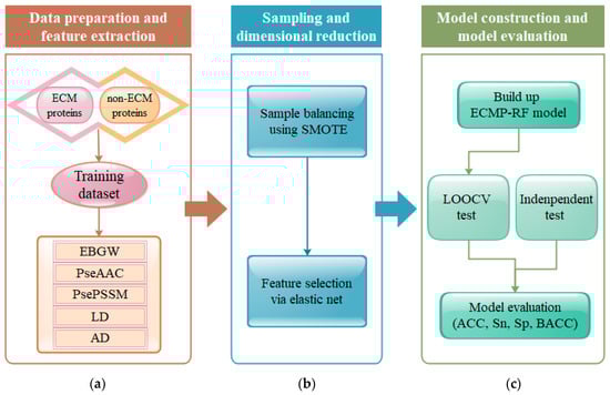
Figure 1.
The flowchart of the ECMP-RF method: (a) data preparation and feature extraction; (b) sampling and dimensional reduction; (c) model construction and model evaluation.
The prediction steps of ECMP-RF are as follows.
- (1)
- Obtain the datasets, and then input the protein sequences of different classes and the corresponding labels.
- (2)
- Feature extraction. Treat protein sequences as special strings, and then convert character signals into numerical signals by encoding as follows: (a) extraction of protein sequence features using PseAAC. (b) feature extraction of protein evolutionary information using PsePSSM. (c) extraction of physicochemical properties of amino acids by EBGW. (d) extraction of physicochemical properties of proteins using AD. (e) extraction of protein sequence information and physicochemical properties using LD. The five extracted features are then fused, and a 1950-dimensional vector space is constructed for each protein sequence in the dataset.
- (3)
- The problem of imbalance in datasets is solved by SMOTE.
- (4)
- Feature selection. The EN is used to remove the redundancy and noise generated by feature fusion, and to screen the optimal feature vector, so as to provide good feature information.
- (5)
- The selected subset of the best features is input into the RF classifier to predict ECM proteins.
- (6)
- Model performance evaluation. ACC, Sn, SP, and BACC are used as evaluation indexes, and the prediction performance of the model is tested by LOOCV.
3. Results
3.1. Selection of Optimal Parameters , , and
The selection of parameters is the core of the prediction model. Extracting effective feature information from protein sequences is a key step in constructing an ECM protein prediction model. In order to obtain better feature information, the parameters need to be continuously adjusted. In this paper, the training dataset was used as the research object to perform feature extraction on protein sequences. The selection of parameters in the PseAAC, in the PsePSSM, and in the AD play an important role in model construction. If ,, and are selected too small, the extracted sequence information is reduced, and it cannot effectively describe the characteristics of protein sequence. If the values of parameters , , and are too large, it causes noise interference and affects the prediction results. In order to find the best parameters, the value was set to 10, 20, 30, 40, and 50, the value was set to 10, 20, 30, 40, and 49, and the value was set to 10, 20, 30, 40, and 50. The RF classifier was used to classify the dataset. ACC, Sn, Sp, and BACC were used as the evaluation indicators. The results were tested by the method of LOOCV. The evaluation values obtained by selecting different parameters in the PseAAC algorithm, PsePSSM algorithm, and AD algorithm are shown in Table 3, Table 4 and Table 5, respectively. The change in BACC value obtained by the feature extraction algorithm upon selecting different parameters is shown in Figure S1 (Supplementary Materials).
Table 3.
The prediction overall accuracy of ECM proteins by selecting different values.
Table 4.
The prediction overall accuracy of ECM proteins by selecting different values.
Table 5.
The prediction overall accuracy of ECM proteins by selecting different values.
The value in PseAAC encoding reflects sequence correlation factors at different levels of amino-acid sequence information. Different values of have different effects on the prediction performance of the model. Considering that the sample sequence length was 50, the values in PseAAC encoding were set to 10, 20, 30, 40, and 50. As can be seen from Table 3, the evaluation indicators changed with . ACC, Sp, and BACC reached the highest when the value of was 20. At this time, the value of ACC was 92.63%, the value of Sn was 12.71%, and the value of BACC was 56.33%. In summary, was selected as the best parameter of PseAAC coding. At this time, the performance of the model was best. When was 20, each protein sequence generated a 40-dimensional feature vector.
Different values of the parameter of the PsePSSM encoding have a certain impact on the prediction performance of the model. Considering that the minimum sample sequence length was 50, the value of parameter in PsePSSM encoding was set to 10, 20, 30, 40, and 49 in this order. It can be seen from Table 4 that the evaluation index changed with the value of . When the value of in the training dataset was 30, the maximum value of BACC was 60.44%, which means that PsePSSM had the best influence on the model performance. Therefore, the value of = 30 was the best parameter in PsePSSM. At this time, each protein sequence generated a 620-dimensional feature vector.
Different values in AD have different effects on the prediction performance of the model. The values in AD were set to 10, 20, 30, 40 and 50 in turn. Table 5 shows that ACC, Sn, Sp, and BACC changed with the change in . When was 20 and 40, the values of ACC, Sp, and BACC in the training dataset slightly decreased, and when was 30, BACC was the highest, reaching 57.63%. When was 30, each protein sequence generated a 630-dimensional feature vector.
3.2. The Effect of Feature Extraction Algorithm on Prediction Results
Extracting protein sequence information using the feature extraction algorithm is an important stage in the construction of ECM protein prediction models. In this paper, five feature extraction algorithms were selected: PseAAC, PsePSSM, EBGW, AD, and LD. In order to better learn the performance of the model, this article made comparisons using five separate feature coding methods and a hybrid feature coding method named ALL (EBGW + PseAAC + PsePSSM + LD + AD). The feature vectors extracted by the six feature extraction methods were input into the RF classifier to predict them respectively. ACC, BACC, Sn, and Sp were used as evaluation indicators to assess the performance of ECMP-RF. LOOCV was used for evaluation. The results predicted by different feature extraction methods are shown in Table 6.
Table 6.
Prediction results of different characteristics of the training dataset.
In the training dataset, the ACC maximum and BACC maximum were 93.62% and 62.76% respectively, which were obtained by the LD algorithm. The ALL feature extraction method obtained an ACC of 95.03%, which was 1.41% to 2.60% higher than the result obtained by a single feature prediction. The BACC was 71.53%, which is 8.77%–15.61% higher than the result obtained by a single feature prediction. The difference in prediction results reflects the effect of feature extraction algorithms on the robustness of the prediction model. The ALL feature extraction method can not only express protein evolutionary information but also effectively use protein physicochemical properties, sequence information, and structure information. Compared with the single feature extraction method, it has better prediction performance.
3.3. Influence of Class Imbalance on Prediction Results
The two datasets used in this article, i.e., the training dataset and testing dataset, were highly imbalanced, with the ratio of positive and negative samples reaching 1:11 and 1:1.5 respectively. In this case, there was a serious imbalance between the dataset categories, and the prediction results of the classifier would be biased toward a large number of categories, which would adversely affect the prediction performance of the model. Therefore, we used SMOTE to improve the generalization ability of model. SMOTE achieves sample balance by deleting or adding some samples. LOOCV and RF classification algorithms were used to test balanced and unbalanced data. The prediction results are shown in Table 7.
Table 7.
The impact of synthetic minority oversampling technique (SMOTE) on the prediction results of the training dataset.
Because of the imbalance of datasets, the evaluation of ACC index was biased. At the same time, the number of non-ECM proteins was much larger than the number of ECM proteins; thus, Sn and SP indexes could not accurately express the performance of the ECMP-RF, while the BACC could reasonably measure the performance of the model in all the above indicators. It can be seen in Table 7 that the dataset processed by SMOTE significantly improved the BACC. On the imbalanced training dataset, the BACC was 71.53%. After the dataset was balanced, the BACC was 97.04%, which is 25.51% higher than before. As a result, we think that, after SMOTE processing, the prediction performance of ECMP-RF was greatly improved.
3.4. The Effect of Feature Selection Algorithm on Prediction Results
Protein sequence features were extracted by EBGW, PseAAC, PsePSSM, LD, and AD feature extraction methods, and a 1950-dimensional feature vector was obtained after fusion. Since the fused feature vector had a large dimension and redundancy, it was very important to eliminate redundant information and keep the effective information of original data. Choosing different feature selection methods had a certain impact on the ACC of ECM protein prediction. To this end, this paper chose seven feature selection methods, namely, PCA, FA, MI, LASSO, KPCA, LR, and EN. RF was used as a classifier, and its results were tested using LOOCV. The optimal feature extraction method was selected by comparing the evaluation indicators. The results obtained by different feature selection methods are shown in Table 8.
Table 8.
Evaluation results of different dimension reduction methods.
Table 8 shows that different feature selection methods had a certain impact on the prediction performance of the model. On the training dataset, the BACC of the EN algorithm was 97.28%, which is 0.11%, 0.16%, 8.14%, 0.12%, 0.10%, and 0.52% higher than that of PCA, FA, MI, LASSO, KPCA, and LR. In addition, ACC, Sn, and SP were 97.28%, 98.78%, and 95.78%, respectively. This shows that, compared with PCA, FA, MI, LASSO, KPCA, and LR, the EN algorithm could effectively select a subset of features, and the prediction effect in the model was better.
From Figure 2, we can see the details of the ROC curve and PR curve of the training dataset under the seven feature selection methods. AUC and AUPR are important evaluation indicators that indicate the classification performance of the model. Higher values of AUC and AUPR denote the better the performance of the model. Results show that the area under the ROC and PR curves predicted by the EN algorithm was the largest. The AUC value was 0.9972, which is 0.02%–14.65% higher than the AUC value obtained by other feature selection methods. The AUPR value was 0.9974, which is 0.02%–6.10% higher than the AUPR value obtained by other feature selection methods. In conclusion, the feature selection result of the EN algorithm was the highest.
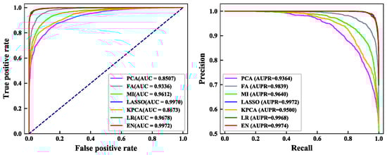
Figure 2.
Comparison of receiver operating characteristic (ROC) and precision recall (PR) curves of seven dimensionality reduction methods. (left) ROC curve of the seven dimensionality reduction methods; (right) PR curve of the seven dimensionality reduction methods.
3.5. The Effect of The Classifier Algorithm on the Prediction Results
Classification algorithms play an important role in building the ECM protein prediction model. In this paper, six common classification algorithms were selected for comparison, namely GBDT, AdaBoost, naïve Bayes, SVM, LR, and RF. The feature subset constructed by EN was input into the six classifiers, and the results were tested by LOOCV. The prediction results of the training dataset on the six classifiers are shown in Table 9. The ROC and PR curves of the six classification algorithms are shown in Figure 3.
Table 9.
Comparison of prediction results of six classifiers.
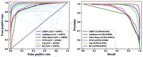
Figure 3.
Comparison of ROC and PR curves of the six classifier algorithms. (left) ROC curve of the six classifier algorithms; (right) PR curve of the six classifier algorithms.
Table 9 shows that, on the training dataset, the BACC obtained by GBDT, AdaBoost, naïve Bayes, SVM, LR, and RF was 83.11%, 93.68%, 83.38%, 84.28%, 91.18%, and 97.28%. Among them, RF’s BACC was 14.17%, 3.60%, 13.90%, 13.00%, and 6.10% higher than that of GBDT, AdaBoost, naïve Bayes, SVM, and LR algorithms. This shows that the classification performance of RF was superior.
It can be seen from Figure 3 that the AUC value of GBDT was 0.9071, the AUC value of AdaBoost was 0.9857, the AUC value of naïve Bayes was the lowest at 0.8822, the AUC value of SVM was 0.9262, the AUC value of LR was 0.9701, and the highest AUC value was achieved by RF at 0.9972. At the same time, the AUPR value of RF also reached 0.9974, which is 1.15%–14.62% higher than that of the other classifiers. Therefore, this paper chose RF as the classifier.
3.6. Comparison with Other Methods
At present, many researchers conducted prediction research on ECM proteins. In order to prove the validity and discrimination of the model, this section compares the ECMP-RF prediction model with other prediction models using the same datasets. To be fair, we use the LOOCV test to compare the expected method with other latest methods on the training dataset and testing dataset.
Figure 4 visually represents the prediction results of ECMP-RF and existing methods on the training dataset. Obviously, of all the methods, ECMPRED had the lowest ACC, Sp, and BACC, while PECMP [24] had the lowest Sn. It is worth noting that, although ECMPP [23] had the highest Sp, its Sn was poor, resulting in poor BACC results. At the same time, the proposed method ECMP-RF could improve the prediction performance of the model and get better results. As the most important evaluation index of the model, BACC was 97.3% in the training dataset. The BACC value of this paper was 19.5% higher than ECMPP, 24.2% higher than PECMP, 26.3% higher than ECMPERD [25], 10.9% higher than IECMP [27], 6.4% higher than ECMP-HybKNN [28], and 3.6% higher than TargetECMP [29]. In addition, the ACC and Sn of ECMP-RF had certain advantages. The comparison results of the training datasets are shown in Table S1 (Supplementary Materials). In short, we conclude that the method we propose is superior to existing models.
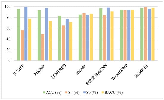
Figure 4.
Comparison of ECMP-RF on training dataset with existing methods.
In order to objectively evaluate the methods proposed in this paper, we used the same testing dataset to test the prediction performance of the above methods. The specific results are shown in Figure 5. The BACC of the testing dataset on ECMP-RF was 97.9%, which is 33.9%, 29.2%, 42.9%, 20.4%, and 11.4% higher than ECMPP [23], PECMP [24], ECMPRED [25], IECMP [27], and TargetECMP [29], respectively. The prediction results show that, compared with other ECM protein prediction methods, the ACC of the ECMP-RF model prediction was much higher than that of other methods, which verifies the excellent performance of ECMP-RF. The comparison results on the testing dataset are presented in Table S2 (Supplementary Materials).
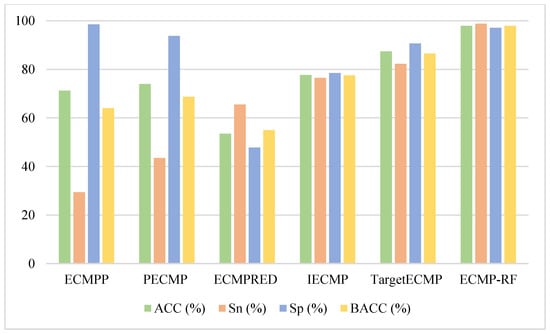
Figure 5.
Comparison of ECMP-RF on testing dataset with existing methods.
4. Discussion
This paper built an ECMP-RF model to predict ECM proteins. PseAAC reflects the sequence information of ECM proteins. EBGW, LD, and AD can effectively extract the physicochemical properties of ECM proteins. PsePSSM extracts evolution information. Feature information is fused, and the SMOTE algorithm is used to solve the problem of data category imbalance. The balanced eigenvector is input into the EN for noise reduction. Using the best feature subset as the input of the RF to predict, ECMP-RF achieves 97.3% BACC in the training dataset through the most rigorous LOOCV, 3.6%–26.3% higher than the existing methods. It also achieves 97.9% BACC in the testing dataset through prediction, 11.4%–42.9% higher than other ECM prediction methods.
- Multi-information fusion can extract protein sequence information more comprehensively and describe protein sequence features in detail compared with single feature extraction method.
- The SMOTE algorithm is used for the first time to solve the problem of data category imbalance and improve the generalization ability of the model.
- Compared with other dimensionality reduction methods, the EN algorithm can effectively remove the redundant information after fusion, and effectively retain the important feature information of ECM protein recognition.
- The RF algorithm used in this paper is an ensemble classification algorithm, which can avoid overfitting and has good prediction performance in proteomics.
Although ECMP-RF improves the accuracy of ECM protein prediction compared with other methods, there is still room for improvement. In future work, we will use deep learning methods to further study ECM protein research, in order to accelerate the speed of model operation and improve the accuracy of the model prediction.
5. Conclusions
ECM proteins participate in a variety of biological processes, and they play an important role in cell life activities. A new prediction method ECMP-RF was proposed in this paper to recognize ECM proteins based on machine learning. The sequence information, evolution information, and physicochemical properties of ECM proteins were considered at the same time. SMOTE was used to solve the problem of class imbalance and avoid prediction bias. EN could effectively remove redundant features while keeping the important features of ECM proteins. The best feature subset was classified and predicted by RF in order to avoid overfitting. Compared with other methods, ECMP-RF advances the research of ECM proteins to a new phase.
Supplementary Materials
The following are available online at https://www.mdpi.com/2227-7390/8/2/169/s1: Figure S1: Change of BACC value corresponding to different parameters of the feature extraction algorithm; Table S1: Comparison of ECMP-RF on training dataset with existing methods; Table S2: Comparison of ECMP-RF on testing dataset with existing methods.
Author Contributions
M.W., L.Y., and B.Y. conceptualized the algorithm, prepared the datasets, carried out experiments, and drafted the manuscript. X.C., C.C., and H.Z. carried out the data coding and data interpretation. Q.M. designed and analyzed the experiments and provided some suggestions for the manuscript writing. All authors read and agreed to the published version of the manuscript.
Funding
This work was supported by the National Nature Science Foundation of China (Nos. 61863010 and 11771188), the Key Research and Development Program of Shandong Province of China (2019GGX101001), and the Natural Science Foundation of Shandong Province of China (No. ZR2018MC007). This work used the Extreme Science and Engineering Discovery Environment, which is supported by the National Science Foundation (No. ACI-1548562).
Conflicts of Interest
The authors declare no conflict of interest.
References
- Campbell, N.E.; Kellenberger, L.; Greenaway, J.; Moorehead, R.A.; Linnerth-Petrik, N.M.; Petrik, J. Extracellular mtrix proteins and tumor angiogenesis. J. Oncol. 2010, 2010, 586905. [Google Scholar] [CrossRef] [PubMed]
- Barkan, D.; Green, J.E.; Chambers, A.F. Extracellular matrix: A gatekeeper in the transition from dormancy to metastatic growth. Eur. J. Cancer 2010, 46, 1181–1188. [Google Scholar] [CrossRef] [PubMed]
- Liotta, L.A. Tumor invasion and extracellular matrix. Lab. Investig. 1983, 49, 636–649. [Google Scholar]
- Adams, J.C.; Watt, F.M. Regulation of development and differentiation by the extracellular matrix. Development 1993, 117, 1183–1198. [Google Scholar]
- Mathews, S.; Bhonde, R.; Gupta, P.K.; Totey, S. Extracellular matrix protein mediated regulation of the osteoblast differentiation of bone marrow derived human mesenchymal stem cells. Differentiation 2012, 84, 185–192. [Google Scholar] [CrossRef]
- Endo, Y.; Ishiwata-Endo, H.; Yamada, K. Extracellular matrix protein anosmin promotes neural grest formation and regulates FGF, BMP, and WNT activities. Dev. Cell 2012, 23, 305–316. [Google Scholar] [CrossRef]
- Kim, S.-H.; Turnbull, J.; Guimond, S. Extracellular matrix and cell signalling: The dynamic cooperation of integrin, proteoglycan and growth factor receptor. J. Endocrinol. 2011, 209, 139–151. [Google Scholar] [CrossRef]
- Aitken, K.J.; Bägli, D.J. The bladder extracellular matrix. Part I: Architecture, development and disease. Nat. Rev. Urol. 2009, 6, 596–611. [Google Scholar] [CrossRef]
- Karsdal, M.A.; Nielsen, M.J.; Sand, J.M.; Henriksen, K.; Genovese, F.; Bay-Jensen, A.C.; Victoria, S.; Adamkewicz, J.I.; Christiansen, C.; Leeming, D.J. Extracellular matrix remodeling: The common denominator in connective tissue diseases possibilities for evaluation and current understanding of the matrix as more than a passive architecture, but a key player in tissue failure. Proteins 2012, 80, 1522–2544. [Google Scholar] [CrossRef]
- Cromar, G.L.; Xiong, X.; Chautard, E.; Ricard-Blum, S.; Parkinson, J. Toward a systems level view of the ECM and related proteins: A framework for the systematic definition and analysis of biological systems. Proteins 2012, 80, 1522–1544. [Google Scholar] [CrossRef]
- Fallon, J.R.; McNally, E.M. Non-Glycanated Biglycan and LTBP4: Leveraging the extracellular matrix for Duchenne Muscular Dystrophy therapeutics. Matrix Biol. 2018, 68–69, 616–627. [Google Scholar] [CrossRef] [PubMed]
- Ma, F.; Tremmel, D.M.; Li, Z.; Lietz, C.B.; Sackett, S.D.; Odorico, J.S.; Li, L. In depth quantification of extracellular matrix proteins from human pancreas. J. Proteome Res. 2019, 18, 3156–3165. [Google Scholar] [CrossRef] [PubMed]
- Gonzalez-Pujana, A.; Santos-Vizcaino, E.; García-Hernando, M.; Hernaez-Estrada, B.; de Pancorbo, M.M.; Benito-Lopez, F.; Igartua, M.; Basabe-Desmonts, L.; Hernandez, R.M. Extracellular matrix protein microarray-based biosensor with single cell resolution: Integrin profiling and characterization of cell-biomaterial interactions. Sens. Actuators B Chem. 2019, 299, 126954. [Google Scholar] [CrossRef]
- Li, Z.C.; Lai, Y.H.; Chen, L.L.; Chen, C.; Xie, Y.; Dai, Z.; Zou, X.Y. Identifying subcellular localizations of mammalian protein complexes based on graph theory with a random forest algorithm. Mol. BioSyst. 2013, 9, 658–667. [Google Scholar] [CrossRef]
- Chen, X.; Chen, M.; Ning, K. BNArray: An R package for constructing gene regulatory networks from microarray data by using Bayesian network. Bioinformatics 2006, 22, 2952–2954. [Google Scholar] [CrossRef][Green Version]
- Tang, Y.R.; Chen, Y.Z.; Canchaya, C.A.; Zhang, Z. GANNPhos: A new phosphorylation site predictor based on a genetic algorithm integrated neural network. Protein Eng. Des. Sel. 2007, 20, 405–412. [Google Scholar] [CrossRef]
- Yamada, K.D.; Omori, S.; Nishi, H.; Miyagi, M. Identification of the sequence determinants of protein N-terminal acetylation through a decision tree approach. BMC Bioinform. 2017, 18, 289. [Google Scholar] [CrossRef]
- Ahmad, K.; Waris, M.; Hayat, M. Prediction of Protein Submitochondrial Locations by Incorporating Dipeptide Composition into Chou’s General Pseudo Amino Acid Composition. J. Membr. Biol. 2016, 249, 293–304. [Google Scholar] [CrossRef]
- Chen, T.Q.; Guestrin, C. XGBoost: A scalable tree boosting system. In Proceedings of the 22nd ACM Sigkdd International Conference on Knowledge Discovery and Data Mining, San Francisco, CA, USA, 13–17 August 2016; pp. 785–794. [Google Scholar]
- Freund, Y.; Schapire, R.E. A decision-theoretic generalization of online learning and an application to boosting. J. Comput. Syst. Sci. 1997, 55, 119–139. [Google Scholar] [CrossRef]
- Wang, B.; Wang, X.F.; Howell, P.; Qian, X.; Huang, K.; Riker, A.I.; Ju, J.; Xi, Y. A personalized microRNA microarray normalization method using a logistic regression model. Bioinformatics 2010, 26, 228–234. [Google Scholar] [CrossRef]
- Friedman, J.H. Greedy function approximation: A gradient boosting machine. Ann. Stat. 2001, 29, 1189–1232. [Google Scholar] [CrossRef]
- Jung, J.; Ryu, T.; Hwang, Y.; Lee, E.; Lee, D. Prediction of extracellular matrix proteins based on distinctive sequence and domain characteristics. J. Comput. Biol. 2010, 17, 97–105. [Google Scholar] [CrossRef] [PubMed]
- Anitha, J.; Rejimoan, R.; Sivakumar, K.C.; Sathish, M. Prediction of extracellular matrix proteins using SVMhmm classifier. IJCA Spec. Issue Adv. Comput. Commun. Technol. HPC Appl. 2012, 1, 7–11. [Google Scholar]
- Kandaswamy, K.K.; Pugalenthi, G.; Kalies, K.U.; Hartmann, E.; Martinetz, T. EcmPred: Prediction of extracellular matrix proteins based on random forest with maximum relevance minimum redundancy feature selection. J. Theor. Biol. 2013, 317, 377–383. [Google Scholar] [CrossRef] [PubMed]
- Zhang, J.; Sun, P.; Zhao, X.; Ma, Z. PECM: Prediction of extracellular matrix proteins using the concept of chou’s pseudo amino acid composition. J. Theor. Biol. 2014, 363, 412–418. [Google Scholar] [CrossRef] [PubMed]
- Yang, R.; Zhang, C.; Gao, R.; Zhang, L. An ensemble method with hybrid features to identify extracellular matrix proteins. PLoS ONE 2015, 10, e0117804. [Google Scholar] [CrossRef]
- Ali, F.; Hayat, M. Machine learning approaches for discrimination of extracellular matrix proteins using hybrid feature space. J. Theor. Biol. 2016, 403, 30–37. [Google Scholar] [CrossRef]
- Kabir, M.; Ahmad, S.; Iqbal, M.; Swati, Z.N.; Liu, Z.; Yu, D.J. Improving prediction of extracellular matrix proteins using evolutionary information via a grey system model and asymmetric under-sampling technique. Chemom. Intell. Lab. 2018, 174, 22–32. [Google Scholar] [CrossRef]
- David, C.C.; Jacobs, D.J. Principal component analysis: A method for determining the essential dynamics of proteins. Methods Mol. Biol. 2013, 1084, 193–226. [Google Scholar]
- Engemann, D.A.; Gramfort, A. Automated model selection in covariance estimation and spatial whitening of MEG and EEG signals. NeuroImage 2015, 108, 328–342. [Google Scholar] [CrossRef]
- Tabbaa, O.P.; Jayaprakash, C. Mutual information and the fidelity of response of gene regulatory models. Phys. Biol. 2014, 11, 046004. [Google Scholar] [CrossRef] [PubMed][Green Version]
- Zou, H. The adaptive lasso and its oracle properties. J. Am. Stat. Assoc. 2006, 101, 1418–1429. [Google Scholar] [CrossRef]
- Li, J.; Li, X.; Tao, D. KPCA for semantic object extraction in images. Pattern Recogn. 2008, 41, 3244–3250. [Google Scholar] [CrossRef]
- Hsieh, F.Y.; Bloch, D.A.; Larsen, M.D. A simple method of sample size calculation for linear and logistic regression. Stat. Med. 1998, 17, 1623–1634. [Google Scholar] [CrossRef]
- Zou, H.; Hastie, T. Regularization and variable selection via the elastic net. J. R. Stat. Soc. Ser. B Stat. Methodol. 2005, 2, 301–320. [Google Scholar] [CrossRef]
- You, Z.H.; Zhu, L.; Zheng, C.H.; Yu, H.J.; Deng, S.P.; Ji, Z. Prediction of protein-protein interactions from amino acid sequences using a novel multi-scale continuous and discontinuous feature set. BMC Bioinform. 2014, 15, S9. [Google Scholar] [CrossRef]
- Zhang, Z.H.; Wang, Z.H.; Zhang, Z.R.; Wang, Y.X. A novel method for apoptosis protein subcellular localization prediction combining encoding based on grouped weight and support vector machine. FEBS Lett. 2006, 580, 6169–6174. [Google Scholar] [CrossRef]
- Wang, X.; Yu, B.; Ma, A.; Chen, C.; Liu, B.; Ma, Q. Protein–protein interaction sites prediction by ensemble random forests with synthetic minority oversampling technique. Bioinformatics 2019, 35, 2395–2402. [Google Scholar] [CrossRef]
- Tian, B.G.; Wu, X.; Chen, C.; Qiu, W.Y.; Ma, Q.; Yu, B. Predicting protein–protein interactions by fusing various Chou’s pseudo components and using wavelet denoising approach. J. Theor. Biol. 2019, 462, 329–346. [Google Scholar] [CrossRef]
- Zhou, H.Y.; Chen, C.; Wang, M.H.; Ma, Q.; Yu, B. Predicting Golgi-resident protein types using conditional covariance minimization with XGBoost based on multiple features fusion. IEEE Access 2019, 7, 144154–144164. [Google Scholar] [CrossRef]
- Yu, B.; Qiu, W.; Chen, C.; Ma, A.; Jiang, J.; Zhou, H.; Ma, Q. SubMito-XGBoost: Predicting protein submitochondrial localization by fusing multiple feature information and eXtreme gradient boosting. Bioinformatics 2019. [Google Scholar] [CrossRef] [PubMed]
- Chou, K.C. Prediction of protein cellular attributes using pseudo-amino acid composition. Proteins 2001, 43, 246–255. [Google Scholar] [CrossRef] [PubMed]
- Cui, X.W.; Yu, Z.M.; Yu, B.; Wang, M.H.; Tian, B.G.; Ma, Q. UbiSitePred: A novel method for improving the accuracy of ubiquitination sites prediction by using LASSO to select the optimal Chou’s pseudo components. Chemom. Intell. Lab. 2019, 184, 28–43. [Google Scholar] [CrossRef]
- Yu, B.; Lou, L.; Li, S.; Zhang, Y.; Qiu, W.; Wu, X.; Wang, M.; Tian, B. Prediction of protein structural class for low-similarity sequences using Chou’s pseudo amino acid composition and wavelet denoising. J. Mol. Graph. Model. 2017, 76, 260–273. [Google Scholar] [CrossRef]
- Butt, A.H.; Rasool, N.; Khan, Y.D. Prediction of antioxidant proteins by incorporating statistical moments based features into Chou’s PseAAC. J. Theor. Biol. 2019, 473, 1–8. [Google Scholar] [CrossRef]
- Yu, B.; Li, S.; Qiu, W.Y.; Wang, M.H.; Du, J.W.; Zhang, Y.S.; Chen, X. Prediction of subcellular location of apoptosis proteins by incorporating PsePSSM and DCCA coefficient based on LFDA dimensionality reduction. BMC Genom. 2018, 19, 478. [Google Scholar] [CrossRef]
- Yu, B.; Li, S.; Qiu, W.Y.; Chen, C.; Chen, R.X.; Wang, L.; Wang, M.H.; Zhang, Y. Accurate prediction of subcellular location of apoptosis proteins combining Chou’s PseAAC and PsePSSM based on wavelet denoising. Oncotarget 2017, 8, 107640–107665. [Google Scholar] [CrossRef]
- Yu, B.; Li, S.; Chen, C.; Xu, J.; Qiu, W.Y.; Chen, R. Prediction subcellular localization of Gram-negative bacterial proteins by support vector machine using wavelet denoising and Chou’s pseudo amino acid composition. Chemom. Intell. Lab. 2017, 167, 102–112. [Google Scholar] [CrossRef]
- Cheng, X.; Xiao, X.; Chou, K.C. pLoc_bal-mPlant: Predict subcellular localization of plant proteins by general PseAAC and balancing training dataset. Curr. Pharm. Des. 2018, 24, 4013–4022. [Google Scholar] [CrossRef]
- Lin, H.; Wang, H.; Ding, H.; Chen, Y.L.; Li, Q.Z. Prediction of subcellular localization of apoptosis protein using chou’s pseudo amino acid composition. Acta Biotheor. 2009, 57, 321–330. [Google Scholar] [CrossRef]
- Jiao, Y.S.; Du, P.F. Predicting Golgi-resident protein types using pseudo amino acid compositions: Approaches with positional specific physicochemical properties. J. Theor. Biol. 2016, 391, 35–42. [Google Scholar] [CrossRef] [PubMed]
- Shen, H.B.; Chou, K.C. Nuc-PLoc: A new web-server for predicting protein subnuclear localization by fusing PseAA composition and PsePSSM. Protein Eng. Des. Sel. 2007, 20, 561–567. [Google Scholar] [CrossRef] [PubMed]
- Qiu, W.Y.; Li, S.; Cui, X.W.; Yu, Z.M.; Wang, M.H.; Du, J.W.; Peng, Y.J.; Yu, B. Predicting protein submitochondrial locations by incorporating the pseudo-position specific scoring matrix into the general Chou’s pseudo-amino acid composition. J. Theor. Biol. 2018, 450, 86–103. [Google Scholar] [CrossRef] [PubMed]
- Shi, H.; Liu, S.; Chen, J.; Li, X.; Ma, Q.; Yu, B. Predicting drug-target interactions using Lasso with random forest based on evolutionary information and chemical structure. Genomics 2019, 111, 1839–1852. [Google Scholar] [CrossRef]
- Chen, C.; Zhang, Q.M.; Ma, Q.; Yu, B. LightGBM-PPI: Predicting protein-protein interactions through LightGBM with multi-information fusion. Chemom. Intell. Lab. 2019, 191, 54–64. [Google Scholar] [CrossRef]
- Chen, Z.; Zhao, P.; Li, F.; Leier, A.; Marquez-Lago, T.T.; Wang, Y.; Webb, G.I.; Smith, A.I.; Daly, R.J.; Chou, K.C.; et al. iFeature: A python package and web server for features extraction and selection from protein and peptide sequences. Bioinformatics 2018, 34, 2499–2502. [Google Scholar] [CrossRef]
- Chawla, N.V.; Bowyer, K.W.; Hall, L.O.; Kegelmeyer, W.P. SMOTE: Synthetic minority over-sampling technique. J. Artif. Intell. Res. 2012, 16, 321–357. [Google Scholar] [CrossRef]
- Blagus, R.; Lusa, L. SMOTE for high-dimensional class-imbalanced data. BMC Bioinform. 2013, 14, 106. [Google Scholar] [CrossRef]
© 2020 by the authors. Licensee MDPI, Basel, Switzerland. This article is an open access article distributed under the terms and conditions of the Creative Commons Attribution (CC BY) license (http://creativecommons.org/licenses/by/4.0/).