Robust Finite-Time Tracking Control for Robotic Manipulators with Time Delay Estimation


Abstract
1. Introduction
2. Preliminaries
2.1. Relative Theorems
- (i)
- V(x) is positive definite in ;
- (ii)
2.2. Problem Formulation
3. Main Results
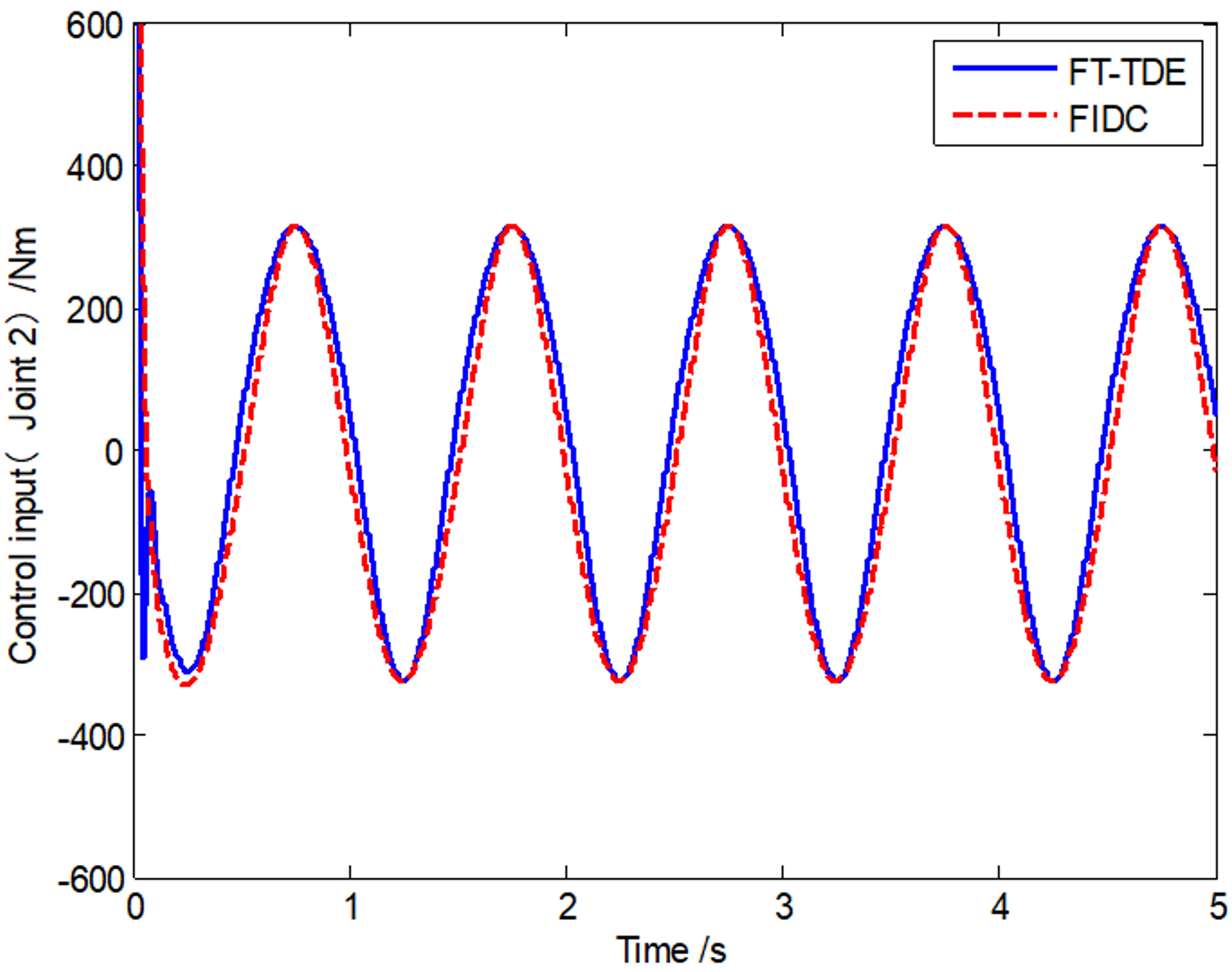
4. Simulations
5. Conclusions
Author Contributions
Funding
Conflicts of Interest
Appendix A
References
- Wang, H. Adaptive Control of Robot Manipulators With Uncertain Kinematics and Dynamics. IEEE Trans. Autom. Control 2017, 62, 948–954. [Google Scholar] [CrossRef]
- Guangjun, L.; Goldenberg, A.A. Robust control of robot manipulators based on dynamics decomposition. IEEE Trans. Robot. Autom. 1997, 13, 783–789. [Google Scholar] [CrossRef]
- Shi, J.; Liu, H.; Bajcinca, N. Robust control of robotic manipulators based on integral sliding mode. Int. J. Control 2008, 81, 1537–1548. [Google Scholar] [CrossRef]
- Haimo, V.T. Finite Time Controllers. SIAM J. Control. Optim. 1986, 24, 760–770. [Google Scholar] [CrossRef]
- Bhat, S.P.; Bernstein, D.S. Finite-time stability of homogeneous systems. In Proceedings of the American Control Conference, Albuquerque, NM, USA, 4–6 June 1997; pp. 2513–2514. [Google Scholar]
- Hong, Y.G. Finite-time stabilization and stabilizability of a class of controllable systems. Syst. Control Lett. 2002, 46, 231–236. [Google Scholar] [CrossRef]
- Huang, X.; Lin, W.; Yang, B. Global finite-time stabilization of a class of uncertain nonlinear systems. Automatica 2005, 41, 881–888. [Google Scholar] [CrossRef]
- Li, J.; Qian, C. Global finite-time stabilization by dynamic output feedback for a class of continuous nonlinear systems. IEEE Trans. Autom. Control 2006, 51, 879–884. [Google Scholar] [CrossRef]
- Zhao, D.; Li, S.; Zhu, Q.; Gao, F. Robust finite-time control approach for robotic manipulators. IET Control Theory Appl. 2010, 4, 1–15. [Google Scholar] [CrossRef]
- Su, Y. Global continuous finite-time tracking of robot manipulators. Int. J. Robust Nonlinear Control 2009, 19, 1871–1885. [Google Scholar] [CrossRef]
- Tang, Y. Terminal sliding mode control for rigid robots. Automatica 1998, 34, 51–56. [Google Scholar] [CrossRef]
- Wu, Y.; Yu, X.; Man, Z. Terminal sliding mode control design for uncertain dynamic systems. Syst. Control Lett. 1998, 34, 281–287. [Google Scholar] [CrossRef]
- Tan, C.P.; Yu, X.; Man, Z. Terminal sliding mode observers for a class of nonlinear systems. Automatica 2010, 46, 1401–1404. [Google Scholar] [CrossRef]
- Feng, Y.; Yu, X.; Man, Z. Non-singular terminal sliding mode control of rigid manipulators. Automatica 2002, 38, 2159–2167. [Google Scholar] [CrossRef]
- Abooee, A.; Moravej Khorasani, M.; Haeri, M. Finite time control of robotic manipulators with position output feedback. Int. J. Robust Nonlinear Control 2017, 27, 2982–2999. [Google Scholar] [CrossRef]
- Ba, D.X.; Yeom, H.; Bae, J. A direct robust nonsingular terminal sliding mode controller based on an adaptive time-delay estimator for servomotor rigid robots. Mechatronics 2019, 59, 82–94. [Google Scholar] [CrossRef]
- Jing, C.; Xu, H.; Niu, X. Adaptive sliding mode disturbance rejection control with prescribed performance for robotic manipulators. ISA Trans. 2019, 91, 41–51. [Google Scholar] [CrossRef]
- Kali, Y.; Saad, M.; Benjelloun, K. Optimal super-twisting algorithm with time delay estimation for robot manipulators based on feedback linearization. Robot. Auton. Syst. 2018, 108, 87–99. [Google Scholar] [CrossRef]
- Kali, Y.; Saad, M.; Benjelloun, K.; Khairallah, C. Super-twisting algorithm with time delay estimation for uncertain robot manipulators. Nonlinear Dynam 2018, 93, 557–569. [Google Scholar] [CrossRef]
- Su, Y.; Zheng, C. Global finite-time inverse tracking control of robot manipulators. Robot. Comput. Integr. Manuf. 2011, 27, 550–557. [Google Scholar] [CrossRef]
- Galicki, M. Finite-time control of robotic manipulators. Automatica 2015, 51, 49–54. [Google Scholar] [CrossRef]
- Liu, H.; Tian, X.; Wang, G.; Zhang, T. Finite-Time H∞ Control for High-Precision Tracking in Robotic Manipulators Using Backstepping Control. IEEE Trans. Ind. Electron. 2016, 63, 5501–5513. [Google Scholar] [CrossRef]
- Lebret, G.; Liu, K.; Lewis, F.L. Dynamic analysis and control of a stewart platform manipulator. J. Robot. Syst. 1993, 10, 629–655. [Google Scholar] [CrossRef]
- Youcef-Toumi, K.; Ito, O. A Time Delay Controller for Systems With Unknown Dynamics. J. Dyn. Syst. Meas. Control 1990, 112, 133–142. [Google Scholar] [CrossRef]
- Khalil, H.K.; Praly, L. High-gain observers in nonlinear feedback control. Int. J. Robust Nonlinear Control 2014, 24, 993–1015. [Google Scholar] [CrossRef]
- Ahrens, J.H.; Khalil, H.K. Output feedback control using high-gain observers in the presence of measurement noise. In Proceedings of the American Control Conference, Boston, MA, USA, 30 June–2 July 2004; Volume 4115, pp. 4114–4119. [Google Scholar]
- Maolin, J.; Jinoh, L.; Pyung Hun, C.; Chintae, C. Practical Nonsingular Terminal Sliding-Mode Control of Robot Manipulators for High-Accuracy Tracking Control. IEEE Trans. Ind. Electron. 2009, 56, 3593–3601. [Google Scholar] [CrossRef]


| r1 (m) | r2(m) | J1(kg⋅m2) | J2(kg⋅m2) | m1(kg) | m2 (kg) | |
|---|---|---|---|---|---|---|
| Actual values | 1 | 0.8 | 5 | 5 | 0.5 | 1.5 |
| Nominal values | 1.2 | 0.9 | 4.5 | 5.1 | 0.6 | 1.3 |
© 2020 by the authors. Licensee MDPI, Basel, Switzerland. This article is an open access article distributed under the terms and conditions of the Creative Commons Attribution (CC BY) license (http://creativecommons.org/licenses/by/4.0/).
Share and Cite
Zhang, T.; Zhang, A. Robust Finite-Time Tracking Control for Robotic Manipulators with Time Delay Estimation. Mathematics 2020, 8, 165. https://doi.org/10.3390/math8020165
Zhang T, Zhang A. Robust Finite-Time Tracking Control for Robotic Manipulators with Time Delay Estimation. Mathematics. 2020; 8(2):165. https://doi.org/10.3390/math8020165
Chicago/Turabian StyleZhang, Tie, and Aimin Zhang. 2020. "Robust Finite-Time Tracking Control for Robotic Manipulators with Time Delay Estimation" Mathematics 8, no. 2: 165. https://doi.org/10.3390/math8020165
APA StyleZhang, T., & Zhang, A. (2020). Robust Finite-Time Tracking Control for Robotic Manipulators with Time Delay Estimation. Mathematics, 8(2), 165. https://doi.org/10.3390/math8020165