Filtering-Based Parameter Identification Methods for Multivariable Stochastic Systems

Abstract
1. Introduction
- The data filtering and model decomposition techniques are used to reduce the computational complexity of the multivariable systems contaminated by uncertain disturbances.
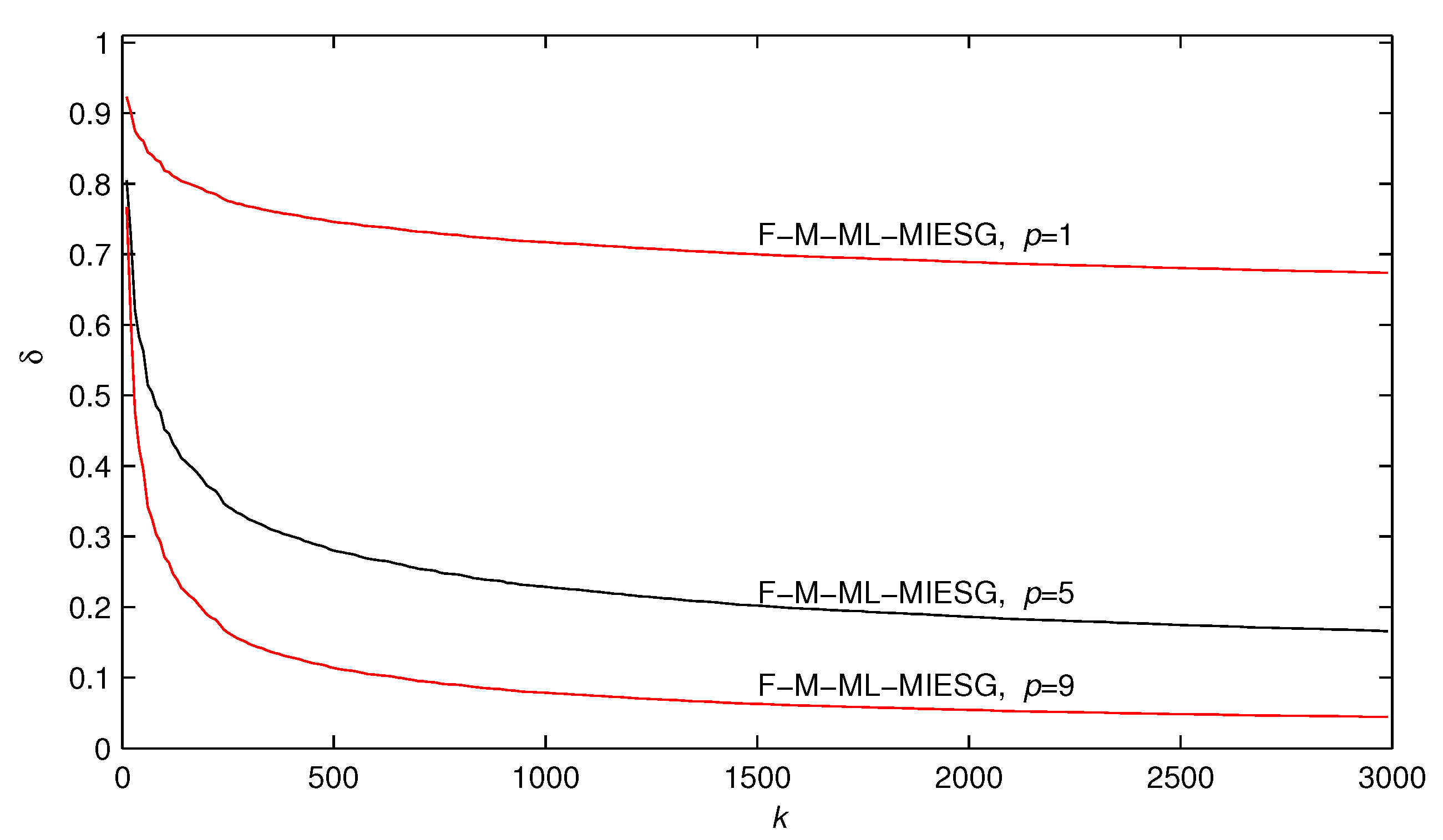
- A filtering-based multivariable maximum likelihood multi-innovation extended stochastic gradient (F-M-ML-MIESG) algorithm is proposed for improved parameter estimation accuracy while retaining desired computational performance.
- The noise model parameters are dealt with directly using the maximum likelihood principle.
2. The System Description and Identification Model
| : | The zero matrix of appropriate sizes. |
| : | An n-dimensional column vector whose entries are all 1. |
| or : | The identity matrix of appropriate sizes or . |
| : | The transpose of the vector or matrix . |
| : | The norm of the vector or matrix . |
| : | X is defined by A. |
| : | X is defined by A. |
| k: | The time variable. |
| : | The estimate of at time k. |
| : | A large positive constant, e.g., . |
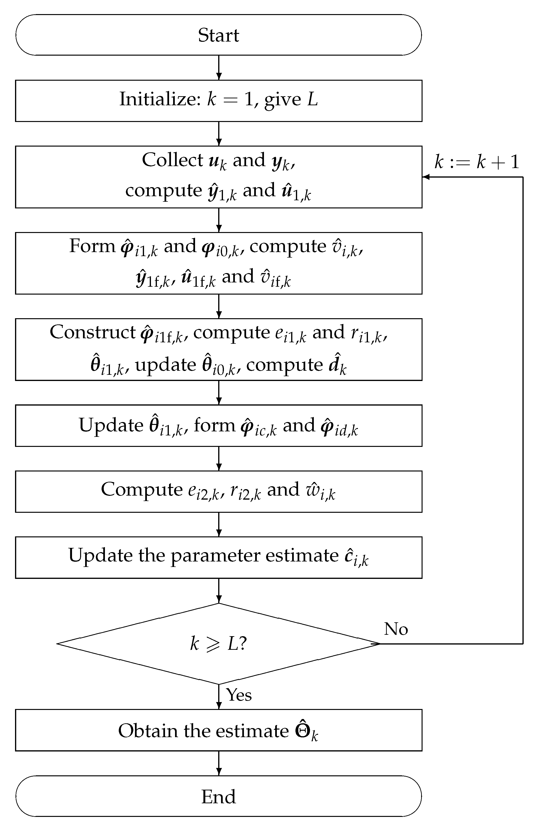
3. The F-M-ML-RESG Algorithm
- Initialization: Let , and set the initial values , , , , , , , , , , and for , .
- Collect and , compute and by (19) and (20), respectively.
- Construct and by (14) and (27), respectively, compute by (12).
- Compute , , and by (16)–(18), respectively, construct by (15).
- Compute and by (10) and (11), respectively.
- Compute by (9), update by (28), compute by (13), update by (29).
- Construct and by (24) and (25), respectively.
- Compute , , and by (22), (23), and (26), respectively.
- Update by (21).
- If , let and go to Step 2; otherwise, terminate this computational procedure and obtain by (30).
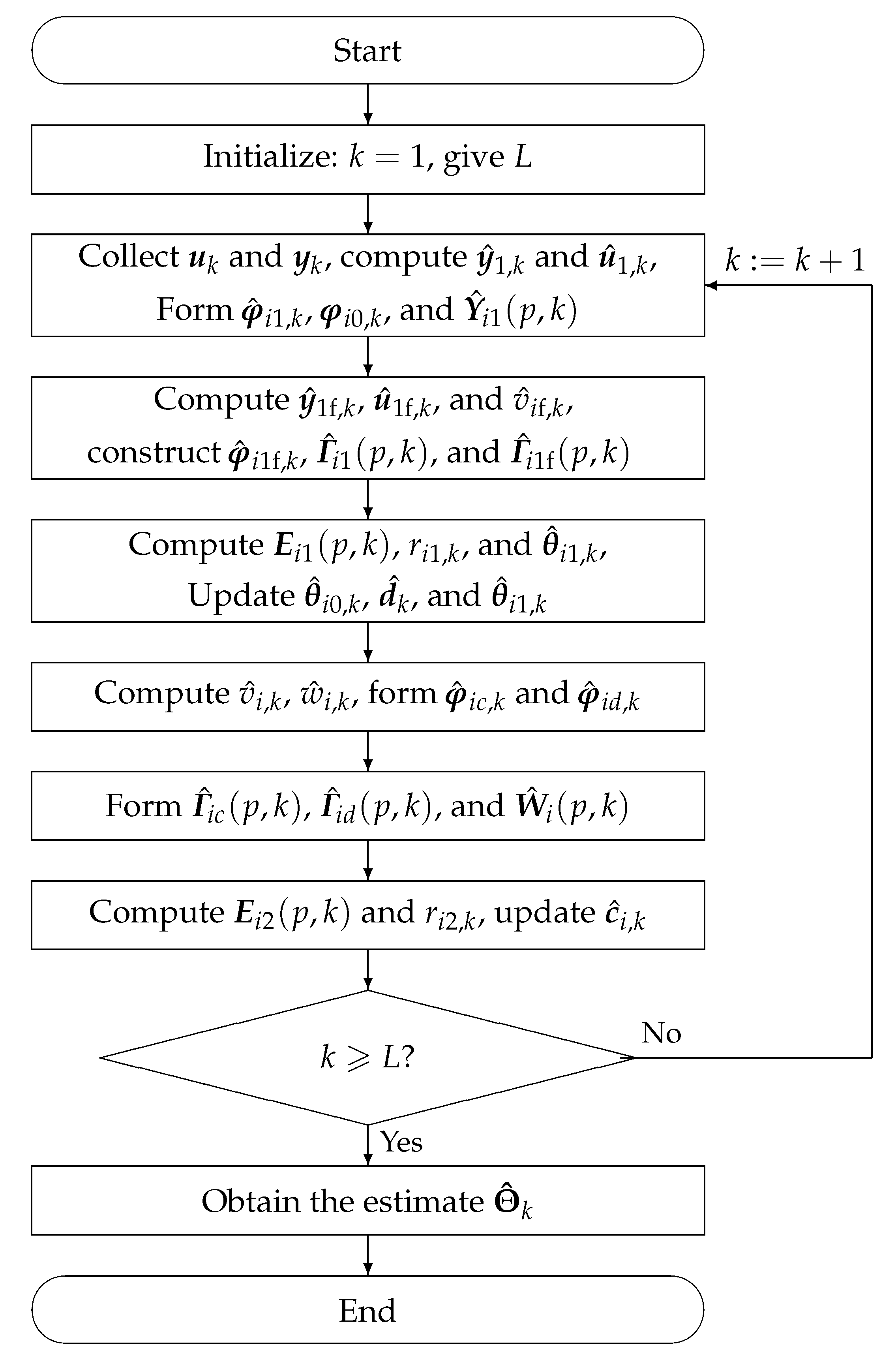
4. The F-M-ML-MIESG Algorithm
- Initialization: Let , and set the initial values , , , , , , , , , , and for , .
- Collect and , compute and by (44) and (45), respectively.
- Form , , and by (39), (55), and (38), respectively.
- Compute , , and by (41)–(43), respectively.
- Form , , and by (40), (36), and (37), respectively.
- Compute , , and by (32), (33), and (31), respectively.
- Update , , and by (56), (35), and (57), respectively.
- Compute and by (34) and (54), respectively.
- Form and by (52) and (53), respectively.
- Form , , and by (49), (50), and (51), respectively.
- Compute and by (47) and (48), respectively.
- Update by (46).
- If , let and go to Step 2; otherwise, terminate this computational procedure and obtain by (58).
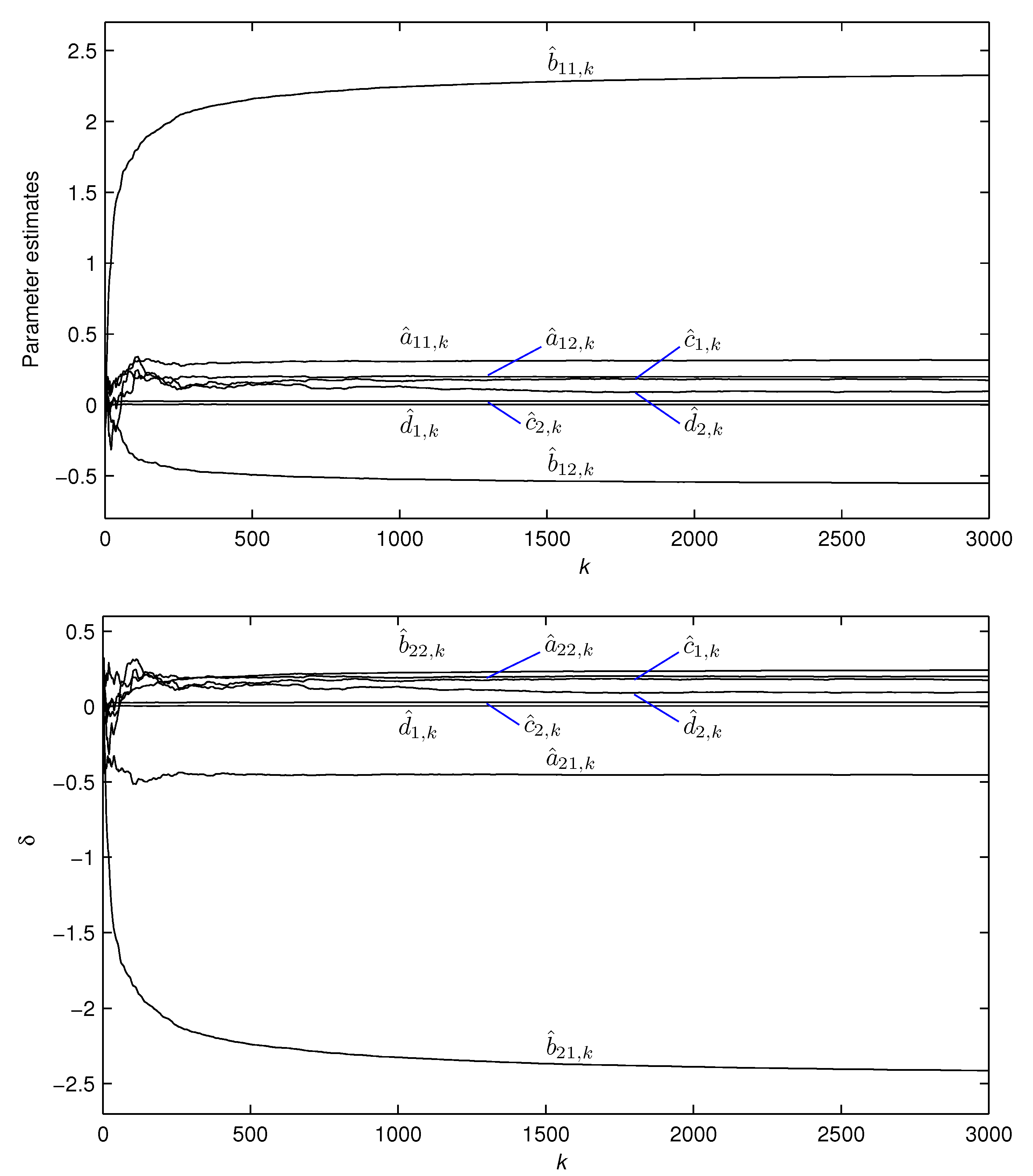
5. Examples
6. Conclusions
Author Contributions
Funding
Conflicts of Interest
References
- Ding, J.; Chen, J.Z.; Lin, J.X.; Wan, L.J. Particle filtering based parameter estimation for systems with output-error type model structures. J. Frankl. Inst. 2019, 356, 5521–5540. [Google Scholar] [CrossRef]
- Xu, L.; Chen, L.; Xiong, W.L. Parameter estimation and controller design for dynamic systems from the step responses based on the Newton iteration. Nonlinear Dyn. 2015, 79, 2155–2163. [Google Scholar] [CrossRef]
- Ding, J.; Chen, J.Z.; Lin, J.X.; Jiang, G.P. Particle filtering-based recursive identification for controlled auto-regressive systems with quantised output. IET Control Theory Appl. 2019, 13, 2181–2187. [Google Scholar] [CrossRef]
- Xu, L. The damping iterative parameter identification method for dynamical systems based on the sine signal measurement. Signal Process 2016, 120, 660–667. [Google Scholar] [CrossRef]
- Ding, J.; Cao, Z.X.; Chen, J.Z.; Jiang, G.P. Weighted parameter estimation for Hammerstein nonlinear ARX systems. Circuits Syst. Signal Process. 2020, 39, 2178–2192. [Google Scholar] [CrossRef]
- Ding, F.; Xu, L.; Meng, D.D.; Jin, X.B.; Alsaedi, A.; Hayat, T. Gradient estimation algorithms for the parameter identification of bilinear systems using the auxiliary model. J. Comput. Appl. Math. 2020, 369, 112575. [Google Scholar] [CrossRef]
- Pan, J.; Jiang, X.; Wan, X.K.; Ding, W. A filtering based multi-innovation extended stochastic gradient algorithm for multivariable control systems. Int. J. Control Autom. Syst. 2017, 15, 1189–1197. [Google Scholar] [CrossRef]
- Zhang, X. Recursive parameter estimation and its convergence for bilinear systems. IET Control Appl. 2020, 14, 677–688. [Google Scholar] [CrossRef]
- Cui, T.; Ding, F.; Alsaedi, A.; Hayat, T. Joint multi-innovation recursive extended least squares parameter and state estimation for a class of state-space systems. Int. J. Control Autom. Syst. 2020, 18, 1412–1424. [Google Scholar] [CrossRef]
- Zhang, X.; Liu, Q.Y. Recursive identification of bilinear time-delay systems through the redundant rule. J. Frankl. Inst. 2020, 357, 726–747. [Google Scholar] [CrossRef]
- Xu, L. Parameter estimation algorithms for dynamical response signals based on the multi-innovation theory and the hierarchical principle. IET Signal Process. 2017, 11, 228–237. [Google Scholar] [CrossRef]
- Bin, M.; Marconi, L. Output regulation by postprocessing internal models for a class of multivariable nonlinear systems. Int. J. Robust Nonlinear Control 2020, 30, 1115–1140. [Google Scholar] [CrossRef]
- Hakimi, A.R.; Binazadeh, T. Sustained oscillations in MIMO nonlinear systems through limit cycle shaping. Int. J. Robust Nonlinear Control 2020, 30, 587–608. [Google Scholar] [CrossRef]
- Cheng, S.; Wei, Y.; Chen, Y.; Wang, Y.; Liang, Q. Fractional-order multivariable composite model reference adaptive control. Int. J. Adapt. Control Signal Process. 2017, 31, 1467–1480. [Google Scholar] [CrossRef]
- Ding, F.; Zhang, X.; Xu, L. The innovation algorithms for multivariable state-space models. Int. J. Adapt. Control Signal Process. 2019, 33, 1601–1608. [Google Scholar] [CrossRef]
- Ding, F.; Liu, Y.J.; Bao, B. Gradient based and least squares based iterative estimation algorithms for multi-input multi-output systems. Proc. Inst. Mech. Eng. Part I J. Syst. Control Eng. 2012, 226, 43–55. [Google Scholar] [CrossRef]
- Ji, Y.; Zhang, C.; Kang, Z.; Yu, T. Parameter estimation for block-oriented nonlinear systems using the key term separation. Int. J. Robust Nonlinear Control 2020, 30, 3727–3752. [Google Scholar] [CrossRef]
- Xia, H.F.; Yang, Y.Q. Maximum likelihood gradient-based iterative estimation for multivariable systems. IET Control Theory Appl. 2019, 13, 1683–1691. [Google Scholar] [CrossRef]
- Zhao, D.; Ding, S.X.; Karimi, H.R.; Li, Y.Y.; Wang, Y.Q. On robust Kalman filter for two-dimensional uncertain linear discrete time-varying systems: A least squares method. Automatica 2019, 99, 203–212. [Google Scholar] [CrossRef]
- Ji, Y.; Jiang, X.K.; Wan, L.J. Hierarchical least squares parameter estimation algorithm for two-input Hammerstein finite impulse response systems. J. Frankl. Inst. 2020, 357, 5019–5032. [Google Scholar] [CrossRef]
- Patel, A.M.; Li, J.K.J.; Finegan, B.; McMurtry, M.S. Aortic pressure estimation using blind identification approach on single input multiple output nonlinear Wiener systems. IEEE Trans. Biomed. Eng. 2018, 65, 1193–1200. [Google Scholar] [CrossRef] [PubMed]
- Tolić, I.; Miličević, K.; Šuvak, N.; Biondić, I. Nonlinear least squares and maximum likelihood estimation of probability density function of cross-border transmission losses. IEEE Trans. Power Syst. 2018, 33, 2230–2238. [Google Scholar] [CrossRef]
- Marey, M.; Mostafa, H. Maximum-likelihood integer frequency offset estimator for alamouti SFBC-OFDM systems. IEEE Commun. Lett. 2020, 24, 777–781. [Google Scholar] [CrossRef]
- Li, M.H.; Liu, X.M. Maximum likelihood least squares based iterative estimation for a class of bilinear systems using the data filtering technique. Int. J. Control Autom. Syst. 2020, 18, 1581–1592. [Google Scholar] [CrossRef]
- Pulido, B.; Zamarreño, J.M.; Merino, A.; Bregon, A. State space neural networks and model-decomposition methods for fault diagnosis of complex industrial systems. Eng. Appl. Artif. Intel. 2019, 79, 67–86. [Google Scholar] [CrossRef]
- Hafezi, Z.; Arefi, M.M. Recursive generalized extended least squares and RML algorithms for identification of bilinear systems with ARMA noise. ISA Trans. 2019, 88, 50–61. [Google Scholar] [CrossRef]
- Boudjedir, C.E.; Boukhetala, D.; Bouri, M. Iterative learning control of multivariable uncertain nonlinear systems with nonrepetitive trajectory. Nonlinear Dyn. 2019, 95, 2197–2208. [Google Scholar] [CrossRef]
- Parigi Polverini, M.; Formentin, S.; Merzagora, L.; Rocco, P. Mixed data-driven and model-based robot implicit force control: A hierarchical approach. IEEE Trans. Control Syst. Technol. 2020, 28, 1258–1271. [Google Scholar] [CrossRef]
- Li, M.H.; Liu, X.M. The least squares based iterative algorithms for parameter estimation of a bilinear system with autoregressive noise using the data filtering technique. Signal Process. 2018, 147, 23–34. [Google Scholar] [CrossRef]
- Xia, H.F.; Yang, Y.Q. Recursive least-squares estimation for multivariable systems based on the maximum likelihood principle. Int. J. Control Autom. Syst. 2020, 18, 503–512. [Google Scholar] [CrossRef]
- Xia, H.F.; Ji, Y.; Yang, Y.Q. Improved least-squares identification for multiple-output nonlinear stochastic systems. IET Control Theory Appl. 2020, 14, 964–971. [Google Scholar] [CrossRef]
- Xia, H.F.; Yang, Y.Q. Maximum likelihood-based recursive least-squares estimation for multivariable systems using the data filtering technique. Int. J. Syst. Sci. 2019, 50, 1121–1135. [Google Scholar] [CrossRef]
- Berntorp, K.; Di Cairano, S. Tire-stiffness and vehicle-state estimation based on noise-adaptive particle filtering. IEEE Trans. Control Syst. Technol. 2019, 27, 1100–1114. [Google Scholar] [CrossRef]
- Ahmad, S.; Rehan, M.; Iqbal, M. Robust generalized filtering of uncertain Lipschitz nonlinear systems under measurement delays. Nonlinear Dyn. 2018, 92, 1567–1582. [Google Scholar] [CrossRef]
- Chen, J.; Zhu, Q.M.; Liu, Y.J. Modified Kalman filtering based multi-step-length gradient iterative algorithm for ARX models with random missing outputs. Automatica 2020, 118, 109034. [Google Scholar] [CrossRef]
- Chen, J.; Shen, Q.Y.; Ma, J.X.; Liu, Y.J. Stochastic average gradient algorithm for multirate FIR models with varying time delays using self-organizing maps. Int. J. Adapt. Control Signal Process. 2020, 34, 955–970. [Google Scholar] [CrossRef]
- Chen, J.; Zhang, Y.; Zhu, Q.M.; Liu, Y.J. Aitken based modified Kalman filtering stochastic gradient algorithm for dual-rate nonlinear models. J. Frankl. Inst. 2019, 356, 4732–4746. [Google Scholar] [CrossRef]
- Ljung, L. System Identification: Theory User, 2nd ed.; Prentice Hall: Englewood Cliffs, NJ, USA, 1999. [Google Scholar]
- Zhang, H.M. Quasi gradient-based inversion-free iterative algorithm for solving a class of the nonlinear matrix equations. Comput. Math. Appl. 2019, 77, 1233–1244. [Google Scholar] [CrossRef]
- Jin, Q.B.; Wang, Z.; Liu, X.P. Auxiliary model-based interval-varying multi-innovation least squares identification for multivariable OE-like systems with scarce measurements. J. Process Control 2015, 35, 154–168. [Google Scholar] [CrossRef]
- Li, J.H.; Zhang, J.L. Maximum likelihood identification of dual-rate Hammerstein output error moving average system. IET Control Theory Appl. 2020, 14, 1078–1090. [Google Scholar] [CrossRef]
- Xia, H.F.; Ji, Y.; Liu, Y.J.; Xu, L. Maximum likelihood-based multi-innovation stochastic gradient method for multivariable systems. Int. J. Control Autom. Syst. 2019, 17, 565–574. [Google Scholar] [CrossRef]
- Xia, H.F.; Ji, Y.; Xu, L.; Alsaedi, A.; Hayat, T. Maximum likelihood-based gradient estimation for multivariable nonlinear systems using the multiinnovation identification theory. Int. J. Robust Nonlinear Control 2020, 30, 5446–5463. [Google Scholar] [CrossRef]
- Dong, S.J.; Yu, L.; Zhang, W.A. Robust hierarchical identification of Wiener systems in the presence of dynamic disturbances. J. Frankl. Inst. 2020, 357, 3809–3834. [Google Scholar] [CrossRef]
- Wang, L.J.; Ji, Y.; Yang, H.L.; Xu, L. Decomposition-based multiinnovation gradient identification algorithms for a special bilinear system based on its input-output representation. Int. J. Robust Nonlinear Control 2020, 30, 3607–3623. [Google Scholar] [CrossRef]
- Xu, L. Iterative parameter estimation for signal models based on measured data. Circuits Syst. Signal Process. 2018, 37, 3046–3069. [Google Scholar] [CrossRef]
- Xu, L.; Xiong, W.L.; Alsaedi, A.; Hayat, T. Hierarchical parameter estimation for the frequency response based on the dynamical window data. Int. J. Control Autom. Syst. 2018, 16, 1756–1764. [Google Scholar] [CrossRef]
- Gu, Y.; Liu, J.; Li, X.; Chou, Y.; Ji, Y. State space model identification of multirate processes with time-delay using the expectation maximization. J. Frankl. Inst. 2019, 356, 1623–1639. [Google Scholar] [CrossRef]
- Xu, L.; Ding, F.; Zhu, Q.M. Hierarchical Newton and least squares iterative estimation algorithm for dynamic systems by transfer functions based on the impulse responses. Int. J. Syst. Sci. 2019, 50, 141–151. [Google Scholar] [CrossRef]
- Xu, L.; Ding, F.; Lu, X.; Wan, L.J.; Sheng, J. Hierarchical multi-innovation generalised extended stochastic gradient methods for multivariable equation-error autoregressive moving average systems. IET Control Theory Appl. 2020, 14, 1276–1286. [Google Scholar] [CrossRef]
- Pan, J.; Ma, H.; Zhang, X.; Liu, Q.Y. Recursive coupled projection algorithms for multivariable output-error-like systems with coloured noises. IET Signal Process. 2020, 14, 455–466. [Google Scholar] [CrossRef]
- Xu, L.; Ding, F.; Wan, L.J.; Sheng, J. Separable multi-innovation stochastic gradient estimation algorithm for the nonlinear dynamic responses of systems. Int. J. Adapt. Control Signal Process. 2020, 34, 937–954. [Google Scholar] [CrossRef]
- Zhang, X.; Ding, F.; Alsaadi, F.E.; Hayat, T. Recursive parameter identification of the dynamical models for bilinear state space systems. Nonlinear Dyn. 2017, 89, 2415–2429. [Google Scholar] [CrossRef]
- Zhang, X.; Xu, L.; Ding, F.; Hayat, T. Combined state and parameter estimation for a bilinear state space system with moving average noise. J. Frankl. Inst. 2018, 355, 3079–3103. [Google Scholar] [CrossRef]
- Gu, Y.; Zhu, Q.; Nouri, H. Bias compensation-based parameter and state estimation for a class of time-delay nonlinear state-space models. IET Control Theory Appl. 2020, 14, 2176–2185. [Google Scholar] [CrossRef]
- Zhang, X.; Ding, F.; Xu, L.; Yang, E.F. State filtering-based least squares parameter estimation for bilinear systems using the hierarchical identification principle. IET Control Theory Appl. 2018, 12, 1704–1713. [Google Scholar] [CrossRef]
- Wang, L.J.; Ji, Y.; Wan, L.J.; Bu, N. Hierarchical recursive generalized extended least squares estimation algorithms for a class of nonlinear stochastic systems with colored noise. J. Frankl. Inst. 2019, 356, 10102–10122. [Google Scholar] [CrossRef]
- Zhang, X.; Ding, F.; Xu, L.; Yang, E.F. Highly computationally efficient state filter based on the delta operator. Int. J. Adapt. Control Signal Process. 2019, 33, 875–889. [Google Scholar] [CrossRef]
- Fan, Y.M.; Liu, X.M. Two-stage auxiliary model gradient-based iterative algorithm for the input nonlinear controlled autoregressive system with variable-gain nonlinearity. Int. J. Robust Nonlinear Control 2020, 30, 5492–5509. [Google Scholar] [CrossRef]
- Zhang, X.; Ding, F.; Yang, E.F. State estimation for bilinear systems through minimizing the covariance matrix of the state estimation errors. Int. J. Adapt. Control Signal Process. 2019, 33, 1157–1173. [Google Scholar] [CrossRef]
- Xu, L.; Song, G.L. A recursive parameter estimation algorithm for modeling signals with multi-frequencies. Circuits Syst. Signal Process. 2020, 39, 4198–4224. [Google Scholar] [CrossRef]
- Gu, Y.; Chou, Y.; Liu, J.; Ji, Y. Moving horizon estimation for multirate systems with time-varying time-delays. J. Frankl. Inst. 2019, 356, 2325–2345. [Google Scholar] [CrossRef]
- Xu, L.; Ding, F.; Yang, E.F. Separable recursive gradient algorithm for dynamical systems based on the impulse response signals. Int. J. Control Autom. Syst. 2020, 18, 3167–3177. [Google Scholar] [CrossRef]
- Zhang, X. Hierarchical parameter and state estimation for bilinear systems. Int. Syst. Sci. 2020, 51, 275–290. [Google Scholar] [CrossRef]
- Gan, M.; Chen, C.L.P.; Chen, G.Y.; Chen, L. On some separated algorithms for separable nonlinear squares problems. IEEE Trans.Cybern. 2018, 48, 2866–2874. [Google Scholar] [CrossRef]
- Zhang, X. Adaptive parameter estimation for a general dynamical system with unknown states. Int. J. Robust Nonlinear Control 2020, 30, 1351–1372. [Google Scholar] [CrossRef]
- Chen, G.Y.; Gan, M.; Chen, C.L.P.; Li, H.X. A regularized variable projection algorithm for separable nonlinear least-squares problems. IEEE Trans. Autom. Control 2019, 64, 526–537. [Google Scholar] [CrossRef]
- Zhang, X.; Ding, F.; Xu, L. Recursive parameter estimation methods and convergence analysis for a special class of nonlinear systems. Int. J. Robust Nonlinear Control 2020, 30, 1373–1393. [Google Scholar] [CrossRef]
- Liu, H.; Zou, Q.X.; Zhang, Z.P. Energy disaggregation of appliances consumptions using ham approach. IEEE Access 2019, 7, 185977–185990. [Google Scholar] [CrossRef]
- Liu, L.J.; Liu, H.B. Data filtering based maximum likelihood gradient estimation algorithms for a multivariate equation-error system with ARMA noise. J. Frankl. Inst. 2020, 357, 5640–5662. [Google Scholar] [CrossRef]
- Wang, L.J.; Guo, J.; Xu, C.; Wu, T.Z.; Lin, H.P. Hybrid model predictive control strategy of supercapacitor energy storage system based on double active bridge. Energies 2019, 12, 2134. [Google Scholar] [CrossRef]
- Tian, S.S.; Zhang, X.X.; Xiao, S.; Zhang, J.; Chen, Q.; Li, Y. Application of C6F12O/CO2 mixture in 10 kV medium-voltage switchgear. IET Sci. Technol. 2019, 13, 1225–1230. [Google Scholar] [CrossRef]
- Ni, J.Y.; Zhang, Y.L. Parameter estimation algorithms of linear systems with time-delays based on the frequency responses and harmonic balances under the multi-frequency sinusoidal signal excitation. Signal Process. 2021, 181, 107904. [Google Scholar] [CrossRef]
- Ji, F.; Liao, L.; Wu, T.Z.; Chang, C.; Wang, M.N. Self-reconfiguration batteries with stable voltage during the full cycle without the DC-DC converter. J. Energy Storage 2020, 28, 101213. [Google Scholar] [CrossRef]
- Wan, X.K.; Jin, Z.Y.; Wu, H.B.; Liu, J.J.; Zhu, B.R.; Xie, H.G. Heartbeat classification algorithm based on one-dimensional convolution neural network. J. Mech. Med. Biol. 2020, 20, 2050046. [Google Scholar] [CrossRef]
- Wan, X.K.; Liu, J.J.; Jin, Z.Y.; Zhu, B.R.; Zhang, M.R. Ventricular repolarization instability quantified by instantaneous frequency of ECG ST intervals. Technol. Health Care 2020. [Google Scholar] [CrossRef]
- Zhang, Y.; Yan, Z.; Zhou, C.C.; Wu, T.Z.; Wang, Y.Y. Capacity allocation of HESS in micro-grid based on ABC algorithm. Int. Low Carbon Technol. 2020, ctaa014. [Google Scholar] [CrossRef]
- Zhao, Z.; Wang, X.; Yao, P.; Bai, Y. A health performance evaluation method of multirotors under wind turbulence. Nonlinear Dyn. 2020, 102, 1701–1715. [Google Scholar] [CrossRef]
- Jin, X.; Wang, H.X.; Wang, X.Y.; Bai, Y.T.; Su, T.L.; Kong, J.L. Deep-learning prediction model with serial two-level decomposition based on bayesian optimization. Complexity 2020, 2020, 4346803. [Google Scholar] [CrossRef]
- Chen, M.T.; Ding, F.; Lin, R.M.; Ng, T.Y.; Zhang, Y.L.; Wei, W. Maximum likelihood least squares-based iterative methods for output-error bilinear-parameter models with colored noises. Int. J. Robust Nonlinear Control 2020, 30, 6262–6280. [Google Scholar] [CrossRef]
- Ma, H.; Pan, J.; Ding, F.; Xu, L.; Ding, W. Partially-coupled least squares based iterative parameter estimation for multi-variable output-error-like autoregressive moving average systems. IET Control Theory Appl. 2019, 13, 3040–3051. [Google Scholar] [CrossRef]


| k | 100 | 200 | 500 | 1000 | 2000 | 3000 | True Values |
|---|---|---|---|---|---|---|---|
| 0.31820 | 0.29087 | 0.30058 | 0.30718 | 0.31435 | 0.31705 | 0.34000 | |
| 0.19071 | 0.19015 | 0.19849 | 0.20414 | 0.19826 | 0.19930 | 0.21000 | |
| −0.49919 | −0.46008 | −0.45017 | −0.45085 | −0.45203 | −0.45256 | −0.47000 | |
| 0.19094 | 0.20269 | 0.19320 | 0.19148 | 0.19971 | 0.19937 | 0.19000 | |
| 1.78343 | 1.97435 | 2.15929 | 2.24258 | 2.30107 | 2.32585 | 2.43000 | |
| −0.36392 | −0.43090 | −0.49287 | −0.52493 | −0.54330 | −0.55194 | −0.59000 | |
| −1.84309 | −2.04914 | −2.23926 | −2.32552 | −2.38841 | −2.41420 | −2.52000 | |
| 0.10917 | 0.16315 | 0.20417 | 0.22542 | 0.23612 | 0.24193 | 0.27000 | |
| 0.19719 | 0.16972 | 0.15718 | 0.16812 | 0.18093 | 0.17411 | 0.18000 | |
| 0.30485 | 0.14739 | 0.13923 | 0.13329 | 0.09666 | 0.09603 | 0.10000 | |
| 0.00360 | 0.00345 | 0.00422 | 0.00412 | 0.00426 | 0.00443 | 0.07000 | |
| 0.02543 | 0.02647 | 0.02684 | 0.02739 | 0.02792 | 0.02811 | 0.12000 | |
| 27.09774 | 18.98626 | 11.36214 | 7.87495 | 5.44330 | 4.46325 |
| k | 100 | 200 | 500 | 1000 | 2000 | 3000 | True Values |
|---|---|---|---|---|---|---|---|
| −0.27269 | −0.32691 | −0.29484 | −0.29755 | −0.29976 | −0.29662 | −0.30000 | |
| 0.48292 | 0.47925 | 0.46018 | 0.45462 | 0.45439 | 0.45430 | 0.45000 | |
| 0.14916 | 0.16587 | 0.20604 | 0.22856 | 0.24342 | 0.24838 | 0.28000 | |
| −0.37780 | −0.36285 | −0.38617 | −0.38781 | −0.39033 | −0.39405 | −0.40000 | |
| 0.12212 | 0.12412 | 0.16615 | 0.18400 | 0.18349 | 0.18549 | 0.20000 | |
| 0.38669 | 0.42406 | 0.44468 | 0.45743 | 0.46705 | 0.47374 | 0.50000 | |
| 0.26876 | 0.24843 | 0.25928 | 0.25579 | 0.25030 | 0.25315 | 0.25000 | |
| 0.31417 | 0.29867 | 0.29703 | 0.29889 | 0.29861 | 0.30047 | 0.30000 | |
| 0.38377 | 0.41180 | 0.43509 | 0.45396 | 0.46774 | 0.47453 | 0.50000 | |
| 0.94218 | 1.05946 | 1.15933 | 1.21302 | 1.25295 | 1.27135 | 1.35000 | |
| −0.62282 | −0.63298 | −0.65448 | −0.66639 | −0.67653 | −0.67960 | −0.70000 | |
| 0.76671 | 0.79860 | 0.82568 | 0.84453 | 0.86025 | 0.86675 | 0.90000 | |
| −1.72820 | −1.88151 | −2.00584 | −2.08070 | −2.13062 | −2.15230 | −2.25000 | |
| 0.96728 | 0.98775 | 1.02537 | 1.04164 | 1.05887 | 1.06517 | 1.10000 | |
| 0.21155 | 0.17143 | 0.14957 | 0.13677 | 0.12570 | 0.12159 | 0.10000 | |
| 0.17930 | 0.21668 | 0.24420 | 0.25904 | 0.27193 | 0.27810 | 0.30000 | |
| 0.01120 | 0.03576 | 0.06050 | 0.07209 | 0.07881 | 0.08311 | 0.10000 | |
| 0.26013 | 0.26116 | 0.27545 | 0.28067 | 0.28621 | 0.28834 | 0.30000 | |
| 0.15333 | 0.21247 | 0.22209 | 0.24500 | 0.20059 | 0.23616 | 0.25000 | |
| −0.02364 | −0.02344 | −0.02373 | −0.02411 | −0.02439 | −0.02471 | −0.10000 | |
| 23.89260 | 17.23794 | 11.32504 | 8.03089 | 5.70767 | 4.79640 |
Publisher’s Note: MDPI stays neutral with regard to jurisdictional claims in published maps and institutional affiliations. |
© 2020 by the authors. Licensee MDPI, Basel, Switzerland. This article is an open access article distributed under the terms and conditions of the Creative Commons Attribution (CC BY) license (http://creativecommons.org/licenses/by/4.0/).
Share and Cite
Xia, H.; Chen, F. Filtering-Based Parameter Identification Methods for Multivariable Stochastic Systems. Mathematics 2020, 8, 2254. https://doi.org/10.3390/math8122254
Xia H, Chen F. Filtering-Based Parameter Identification Methods for Multivariable Stochastic Systems. Mathematics. 2020; 8(12):2254. https://doi.org/10.3390/math8122254
Chicago/Turabian StyleXia, Huafeng, and Feiyan Chen. 2020. "Filtering-Based Parameter Identification Methods for Multivariable Stochastic Systems" Mathematics 8, no. 12: 2254. https://doi.org/10.3390/math8122254
APA StyleXia, H., & Chen, F. (2020). Filtering-Based Parameter Identification Methods for Multivariable Stochastic Systems. Mathematics, 8(12), 2254. https://doi.org/10.3390/math8122254