1. Introduction
The growing data availability, and widespread monitoring systems, have boosted the focus on urban traffic analysis and vehicle movement observation. The study of spatial-temporal transit volume distribution in urban environments is a central aspect for guiding decision-making processes according to the current traffic situation, and can be approached in several different modalities and in a wide variety of contexts [
1,
2]. Typical applications include traffic congestion warnings [
3,
4], car accident risk assessments [
5,
6], and pollution measurement estimations [
7,
8].
In this context, the focus on predictive analytics is prominent, and a number of works dealing with traffic forecasting can be enumerated [
9,
10,
11,
12,
13,
14]. Vehicle-related predictions have been widely approached under different concepts, definitions, and assumptions, becoming a very active research area in the big picture of location-based services and smart city features. A general forecasting direction addresses the inference of the amount of active vehicles located in a specific area at some point in the future, based on the present volume, past trend variations, and additional side information, if available. Depending on the background, this may embody into very different problems and approaches, comprising the identification of congestion locations [
15,
16,
17], traffic estimations of road tracts [
18,
19,
20], and individual vehicle movement predictions [
21,
22,
23].
Our paper tackles a particular case, focusing on the problem of predicting the number of vehicles moving across several urban regions. In contrast with many works analyzing traffic flow in a single selected geographic point (e.g., [
24,
25,
26,
27]), we open to concurrent predictions on multiple flows, considering different reference points (and directions) connecting city areas, therefore providing an estimated future distribution of vehicles across different locations of interest over the territory. Moreover, we concentrate upon short-term predictions, namely forecasting the transit volume according to an hourly time step. Since traffic volume is subject to rapid changes in time and space, the main challenge lies in grasping abrupt variations beyond the general trend.
Predicting short-term distribution of vehicles across the city is indeed of great importance for urban traffic control, particularly in the context of smart city services for nearly real-time decision-making outcomes and intelligent information retrieval [
28,
29]. Estimations on the number of vehicles entering and leaving a city, or moving between urban areas, gives a valuable indication on potential localized bottlenecks and congestions. Inserted in the big wave of mobility mining [
30,
31] heading to providing valuable knowledge on human mobility and urban travel behaviors, the possibility of predicting urban vehicle flows is highly beneficial for timely traffic management strategies, targeted congestion warnings, and any required general forestalling action.
Our case study targets urban toll plazas in correspondence with the Metropolitan Transportation Authority (MTA) tunnels and bridges in New York City, which, serving over 900,000 vehicles per day, carry more traffic than any bridge and tunnel complex in the USA [
32]. Focusing on large urban contexts in the presence of high transit volumes, we propose a geographically-oriented short-term forecasting methodology to predict vehicles’ distribution over the territory, leveraging sequential modeling and deep neural networks.
The underlying assumption is built on successfully mining temporal patterns of traffic volumes, embodying the hypothesis that the current number of registered moving vehicles exhibits some dependences on past measured quantities. The characteristic features in the series are therefore assumed to carry essential information for anticipating future vehicles’ distribution. While typical time series forecasting focus on learning the general trend via purely statistical methods [
33,
34,
35,
36], the natural characterization of our short-term predictive analysis is defined by rapid and steep variations that need to be properly detected in order to provide accurate estimations. Smoothing the phenomena with regressive statistical models tends to lead to ineffective predictions, when in the presence of intense oscillations and shifts to boundary conditions [
37,
38,
39]. Moreover, since multiple traffic flows are taken into account, multiple predictions are to be performed, whereby each reference point (and direction) on the territory is associated to different traffic volumes and different sequential patterns over time. Our goal is to collectively generate accurate predictions based upon a single model (and a single training process) comprising the totality of reference points, therefore following an efficient strategy and avoiding singularly fitting each selected traffic direction with its corresponding distinctive model (as it is required for statistical approaches). Furthermore, this way leverages a combined global view of the city trend, not only analyzing patterns of single geographic directions, but also detecting inter-location relations in the traffic variation.
In an attempt to satisfy the above-mentioned requirements in a straightforward and effective modality, we propose a multi-target deep learning regressor, trained on location-specific time series, for simultaneous predictions of traffic volumes in multiple entry and exit points among city neighborhoods. By leveraging a single training process for all location points and an instant one-step volume inference for every location at each time update, our sequential modeling approach is able to grasp rapid variations in the time series and process the collective information of all reference points, whose distinct predicted values are outputted at once. Firstly, sequences of numbers of vehicles are considered, whereby each selected geographic point on the territory is represented by a series of values unfolding in a fixed time step. Then, the sequences are stacked together as a combined input to a long short-term memory (LSTM) recurrent network-based regressor, which is jointly trained on the block of time series to learn the underlying patterns of urban traffic flows. Finally, a multi-target dense layer provides a number of output values equal to the number of reference locations (and directions). The suggested approach is purely data-driven, capturing variability patterns directly from traffic volume sequences, without any manual feature extraction.
The main contribution of the paper therefore stands out as an extensive exploration of multi-target artificial neural networks for promisingly handle multiple traffic series belonging to spatially-related reference points, arranging a collective processing of multiple input sequences into corresponding multiple forecasted output values. Falling in the context of deep learning applications on human mobility analysis, the underlying purpose is to extend a purely data-driven perspective on vehicle number forecasting for an improved quality of urban management and organization.
The structure of the paper is arranged as follows:
Section 2 describes the methodological workflow supporting the prediction task, specifically illustrating the data pre-processing (
Section 2.1), the model architecture (
Section 2.2), and the model training (
Section 2.3);
Section 3 concerns the experimental arrangement, presenting the dataset (
Section 3.1), the general set-up (
Section 3.2), and the achieved results (
Section 3.3);
Section 4 finally reports the discussion and conclusion.
2. Methodology
The proposed forecasting method aims to collectively learn sequential patterns of spatial-temporal traffic volume variation, specifically predicting the future number of vehicles crossing each of many selected reference locations. Given a stacked input block of multiple time series (each referring to a specific reference location) sampled at a fixed coordinated time step, the solution of our model consists of inferring the vehicles’ distribution over the territory during the next time step in the future. The current section reports the overall methodological description, from collective time series definition to sequential multi-target deep learning modeling.
2.1. Time Series Data Structure
The methodology follows a sequential modeling approach, leveraging a collection of historical time series, each referring to a specific reference location over the territory.
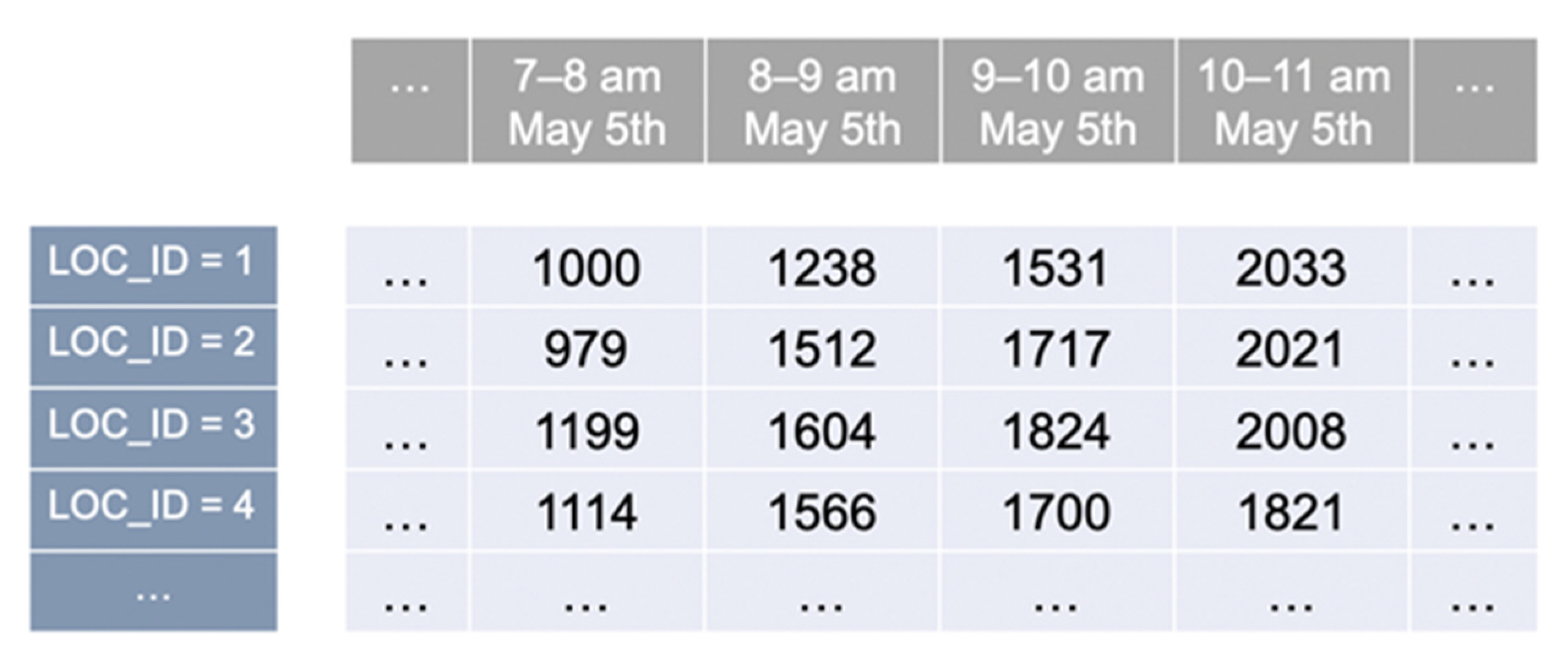
A time series is defined as a sequence of real values unfolding into a predefined time step. If data are not originally sequentially structured (e.g., still in the raw form of individual vehicle recordings), they require to be reshaped into a series of vehicle counts by transforming the continuity of time into fixed time steps and counting the total number of vehicles crossing the reference location within each time span . Each location is therefore described as a series of chronologically ordered vehicle counts .
The sequences of all locations are then stacked together, synchronized at the same time step. The input to the prediction model becomes a time series of multiple dimensions, where the dimensionality is equal to the number of reference locations. In particular, given a number of
locations, the portion of the sequence identified by a specific time span
is made of a vector of
values reporting the number of vehicles within the time span
in each location
, namely
. Therefore, the same longitudinal position along the stacked sequence identifies locations’ count values that are referring to the same time span, as shown in
Figure 1. The length of the time step is case specific, its choice depends on the data source and the prediction problem; our focus specifically relies on short-term forecasting of rapid sequential variations. Analogously, different datasets leverage different numbers of reference locations within the same general phenomenon.
In any case, the data configuration should consist of a set of reference points over the territory, each of them described by a specific time series made of sequential counts of recorded vehicles in consecutive time spans. The final input to the model is then arranged as a block of these series, stacked together on the longitudinal dimension, unfolding in the same identical time steps.
2.2. Multi-Target Deep Learning Model for Distributed Traffic Prediction
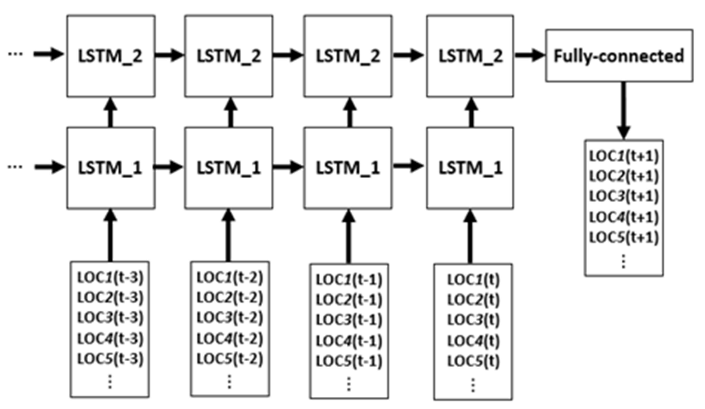
The collection of stacked location-specific time series is defined as the input data to the deep neural network model, whose processing workflow can be depicted according to its three structural components: a multi-dimensional input layer, a block of LSTM recurrent network layers, and a multi-target output layer. A high-level visual overview of the modeling conceptual architecture is reported in
Figure 2. The following subsections singularly focus on each of the three parts composing the model.
2.2.1. Input Layer
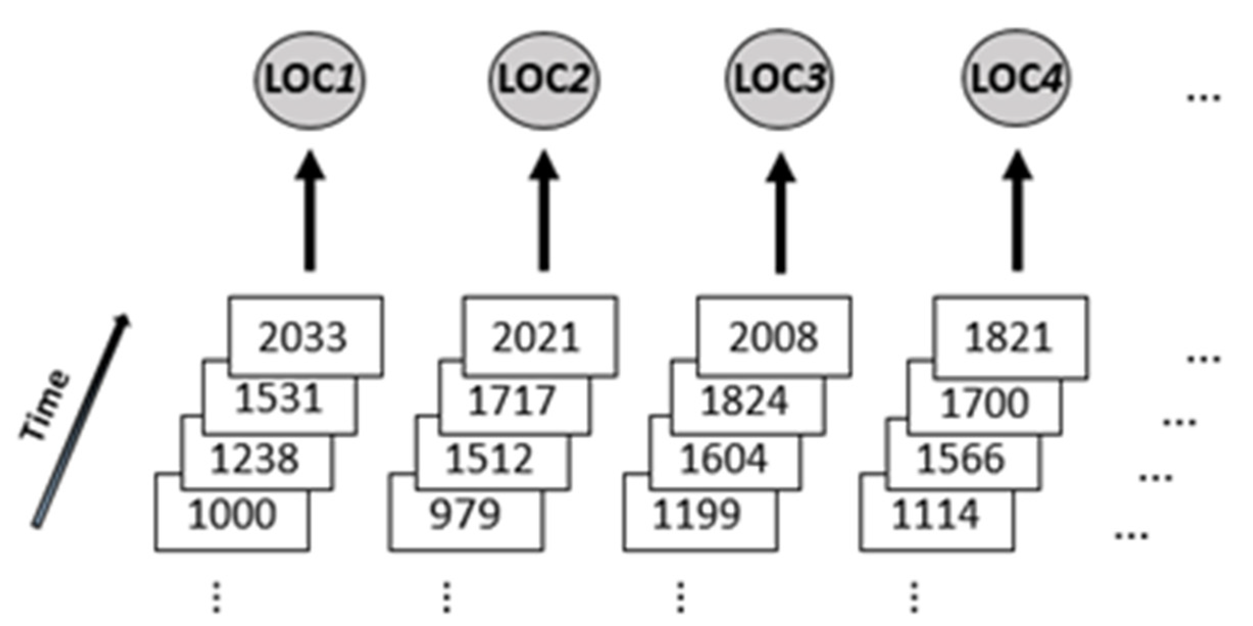
To collectively handle multiple time series with a single model, while still retaining individual characteristics, we make use of a multi-dimensional input layer, whereby each input neuron refers to a specific reference location. Sequences are therefore processed simultaneously but initially addressed through separate channels. A number of
reference vehicle flows identify
time series, which are combined into a sequence of
dimensions, input for a layer of
neurons. At each time step, the model is fed with a vector of
values, one for each reference location; over new consecutive steps, the values referring to a same location always occupy the same position in the array. This means to automatically get the collection of traffic volumes for all the areas at once, but heading to separate input neurons, as reported in
Figure 3. In general, two input processing perspectives are present: the sequential time-dependent evolution of the series, and the horizontal traffic distribution over multiple location points. During the training process, the model receives consecutive chronologically-ordered vectors of size
, and accordingly defines the updates to the parameters of the recurrent and output layers.
2.2.2. LSTM Block
The automatic pattern learning activity is conducted by a recurrent network block, leveraging LSTM layers. LSTM [
40] is a complex recurrent module, composed of four distinctive neural networks interacting between each other. Due to the characteristic capability of handling sequential data, it has been utilized in a variety of applications dealing with motion trajectory prediction [
41,
42,
43] and mobility-related time series forecasting [
44,
45,
46]. A few adoptions to studies on traffic analysis are also present, but has been mainly modeled for singularly predicting flows on a selected target location [
47,
48,
49,
50].
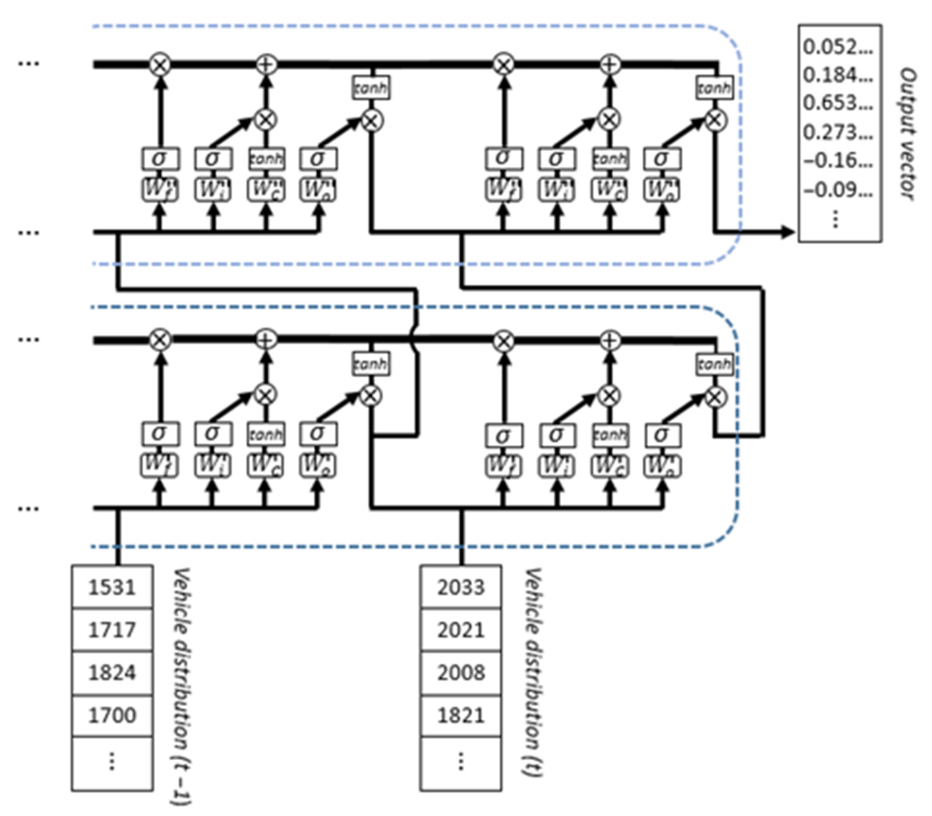
The functioning of an LSTM cell consists of processing sequential data one element at a time, receiving, at each step, two input sources: the current input data element and the processed network output of the previous time step. The encoded information, repeatedly modified by the four internal neural network structures, is defined in the form of a cell state vector. In the last processing step preceding prediction, this evolves into an output vector carrying the overall compressed characterization of the series, subsequently used for disclosing the explicit prediction outcome.
Examining the process from our perspective, the recurring input to the LSTM is represented, at each time step, by the current distributed vector representation along the multi-dimensional sequence of traffic volume, concatenated with the output vector of the LSTM module at the previous step. As a result of the network structure, the cell state contains the pattern information of all reference locations together, encoded in a single vector representation. Therefore, even if different locations initially targeted different entry channels, their single peculiarities are then mixed up in the LSTM state vector and, consequently, in the final output characterization. If the LSTM block contains multiple LSTM layers, the first layer is fed with the input data, the second layer is fed with the output of the first layer, and so on; the final output vector refers to the last step of the last layer.
Figure 4 visually reports the last two steps of a sequence of vehicle flows, processed by a recurrent block of two LSTM layers.
Equations (1)–(6) describe a repeating module of LSTM in further detail. Considering a sequence
and an input vector
at time
, the forget gate (1) is intended to selectively erase information; the input gate (2) is oriented to indicate which values are required to be updated; the tanh network (3) aims to provide novel information in the form a vector of new candidate values; the cell state (4) is therefore updated following a filtering action through the forget gate and adding up with the combined outcome of the input gate and the tanh network; the output gate (5) is then arranged to select which parts of the cell state to output; and finally, the LSTM outcome (6) derives from the multiplication of the output gate with the tanh of the updated cell state.
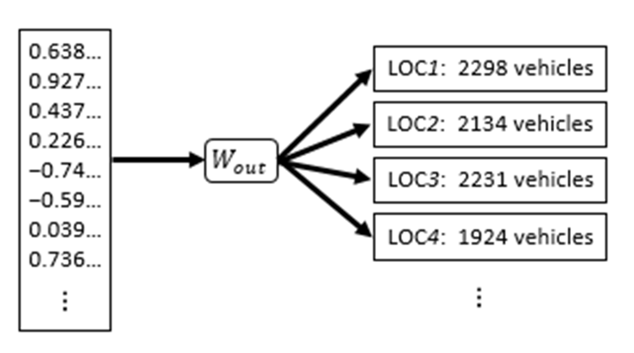
2.2.3. Output Layer
The output layer is intended to sustain the function of translating the LSTM final vector representation into the explicit traffic volume distribution across the different reference locations. The task relies on providing a number of output values equal to the number of locations. In particular, each output neuron is required to predict the future number of vehicles crossing a single specific reference point, therefore depicting the forecasting process as a multi-target regression analysis.
The layer consists of a multi-output fully-connected neural network on top of the LSTM block. Its purpose is to transform the compressed encoded information, contained in a single dense vector, into multiple simultaneous predictions conforming to the distributed geographic perspective, as reported in
Figure 5.
Equation (7) formally describes the output layer, where
indicates the total number of reference locations and
refers to the final vector representation of the LSTM block.
2.3. Model Training
The procedure of identifying, at each time step, the input data elements and the corresponding target value for training the model is accomplished by scanning the multi-dimensional sequence of vehicle distribution with a sliding window, which, consecutively moving forward by one step until the end of the sequence, produces multiple input segments of a fixed length. The segment length defines the extent of the continuous sequential dependencies grasped through pattern mining, and is strongly influenced by the data characteristics. Its choice may vary according to different experimental setups and time resolutions, even within the same domain analysis.
The sequential learning of traffic evolution is driven by such collection of segments, characterizing a training process based on input sequences paired with their corresponding future target values. The parameter optimization focuses on minimizing the mean squared error between the predicted amounts of vehicles and the actual recorded numbers. The weights within every layer of the network are therefore updated through a backpropagation process and mini-batch stochastic training, gradually adjusted towards the direction of the gradient to provide more and more accurate prediction outputs, with respect to the real target volumes.
At testing time, the learned parameter configuration, based on historical pattern mining, allows for predicting the traffic distribution in the future. The instant forecasting of the distributed number of vehicles across the territory is therefore grounded on the model’s detection, in the time span preceding prediction, of sequential patterns that resemble past traffic variability tendencies.
3. Experiment
We hereby provide a description of the experimental settings and the evaluation dataset, followed by an overview of the results and findings on the forecasted traffic volume distribution within a real-world environment. The deep learning model was implemented and trained using TensorFlow, and subsequently evaluated in relation to multiple baseline performances for a proper measure of its feasibility.
3.1. Dataset
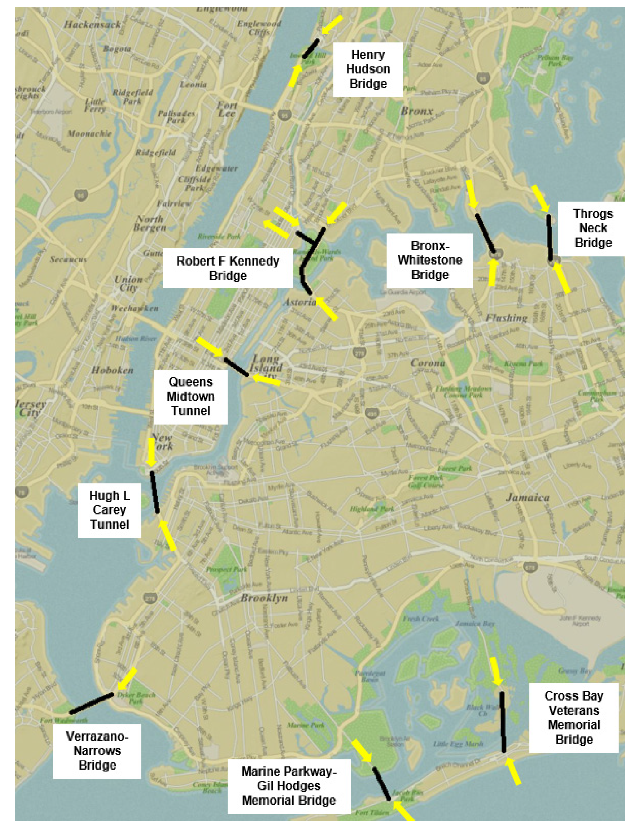
The experimental analysis on future traffic distributions across urban regions leverages a real-world dataset of hourly counts of vehicles crossing several entry and exit reference points between city neighborhoods. Specifically, the data refer to the urban toll plazas in correspondence of the nine MTA tunnels and bridges in New York City [
32], depicting an exemplifying case study of large urban context in the presence of high transit volumes. In particular, we analyzed the time span from January 2012 to December 2015, targeting a total of 19 different vehicle flow directions, as represented in
Figure 6. A single observation includes the plaza identifier, the transit direction, the date and hour, and the number of observed vehicles.
The model input consists of a 19-dimensional sequence, describing the traffic volume variation over time for each of the reference locations. The sequence unfolds in hourly time steps, whereby a single step reports the total number of vehicles in the last hour, distributed over multiple geographic points. This multi-location perspective therefore identifies each new input element as a vector of 19 values, representation of the current hourly distribution of traffic volume across city neighborhoods’ connecting routes.
3.2. Experimental Settings
The neural network model architecture was designed with a block made of two LSTM layers, characterized by a hidden size of 128 neurons each. The sliding window progressively collecting the scaled input values was set to include the 12 h before prediction, and the forecasting output format was defined as a vector of 19 dimensions, reporting the predicted number of vehicles crossing each of the reference locations in the following hour. The mini-batch stochastic training process featured a parameter configuration update based on the mean squared error loss function and Adam optimizer [
51]. The outcome was finally assessed on a data portion that was not involved in the training phase; specifically, three consecutive years were chosen as a training set (2012–2014), and the successive year (2015) was selected as testing data for evaluating the model.
Global measures, to quantify the overall performance, were based on the prevalent metrics of mean squared error (MSE), root mean squared error (RMSE), and mean absolute error (MAE). Separate results on the single reference locations were also taken into account, to assess some possible geographic inhomogeneity in the forecasting outcomes.
For a meaningful reasoning on the quality of our methodology, the performance evaluation was compared to baseline approaches comprising cyclical mining of historical recurrent trends and regressive statistical modeling, typical methods for time series analysis. The next subsection reports the experimental results and examines the findings deriving from the predicted vehicle distribution across the multiple selected reference directions.
3.3. Results
The global scores in terms of MSE, RMSE and MAE are reported in
Table 1. The multi-target LSTM model is compared with baselines built on the concept of cyclical repeating patterns or steady behaviors in time, aiming to quantify its performance advantage over rule-based approaches highlighting particular specific characteristics of the sequential phenomena. Specifically, four baselines were selected, each focusing on a particular aspect of traffic flow dynamics. A first approach (“Last hour”) models steady behaviors, assuming little changes on consecutive hours, therefore predicting the number of vehicles as the same of the number registered in the previous hour. A second baseline (“Daily cycle”) depicts daily cyclical recurrences, assuming the prediction outcome as equal to the number of vehicles observed at the same hour of the previous day. A third baseline (“Weekly cycle”) focuses instead on weekly cycles, expecting the future volume to be equal to the number of vehicles of the previous week, in the same day of the week and at the same time, hypothesizing a general weekly repetitiveness of the trends. The fourth baseline (“Weekly cycle (4 weeks avg)”) is a generalization of the third one, applying the same principle but, instead of only focusing on the previous week, it takes into account the whole previous month, averaging the corresponding weekly values (e.g., the traffic volume on the next Monday at 6pm is forecasted as the average of the past four Mondays at 6 pm) and, therefore, reducing fluctuation noises along the sequence. Finally, we set two further baselines in the form of regressive statistical methods for time series analysis, fitting each series with the commonly utilized ARIMA and FBprophet models, widely-adopted performance thresholds for series-related comparative analysis, due to their widespread and efficient automatic implementations of parameter tuning.
The results report the best baseline to be the monthly-averaged weekly cycle-based approach, enhancing a weekly recurrent characteristic pattern. On the other hand, our model is shown to substantially outperform the baselines, pointing out a remarkable forecasting capability, disclosing a MSE of 26K versus the best baselines’ value of 72K.
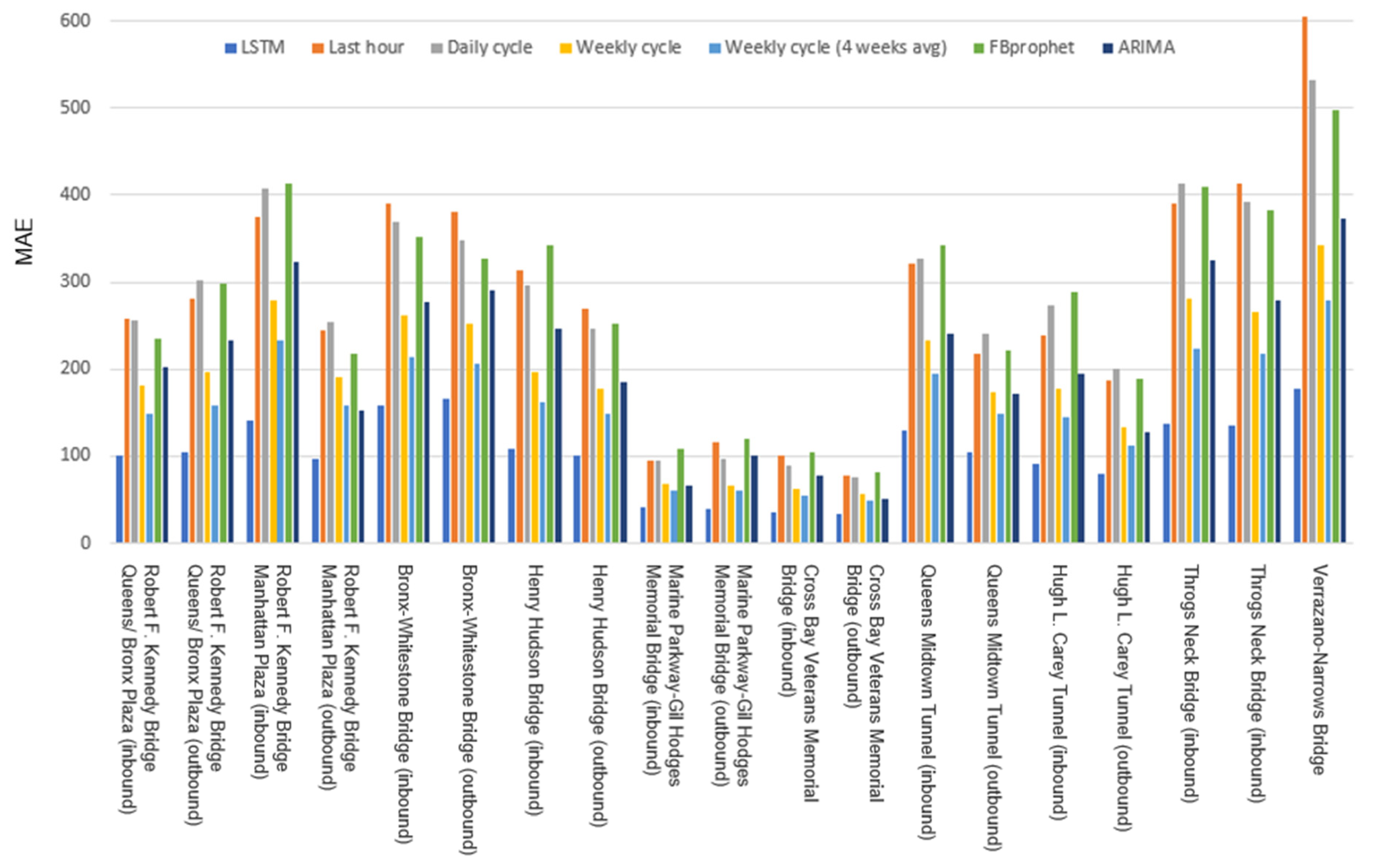
Referring only to a global mean score may not be fully revealing because of the diverse quantities of traffic volume in correspondence of different reference locations, which consequently leads to various distinctive degrees of prediction error.
Figure 7, therefore, provides a complete overview of the MAE distribution over the multitude of reference points. Specifically, the distributed outcome of the LSTM model is compared to the baselines with respect to each of the 19 traffic flows under study, revealing a superior performance in all of them, regardless of any difference in the local traffic amounts. The best baseline is confirmed to be the same for the great majority of reference directions, whereas the sequential statistical processes are not able to catch the rapid variations in the series, ending up in a widespread poor fitting performance (combined with the inefficiency of requiring a separate fit for each single flow, not handling any multi-output option).
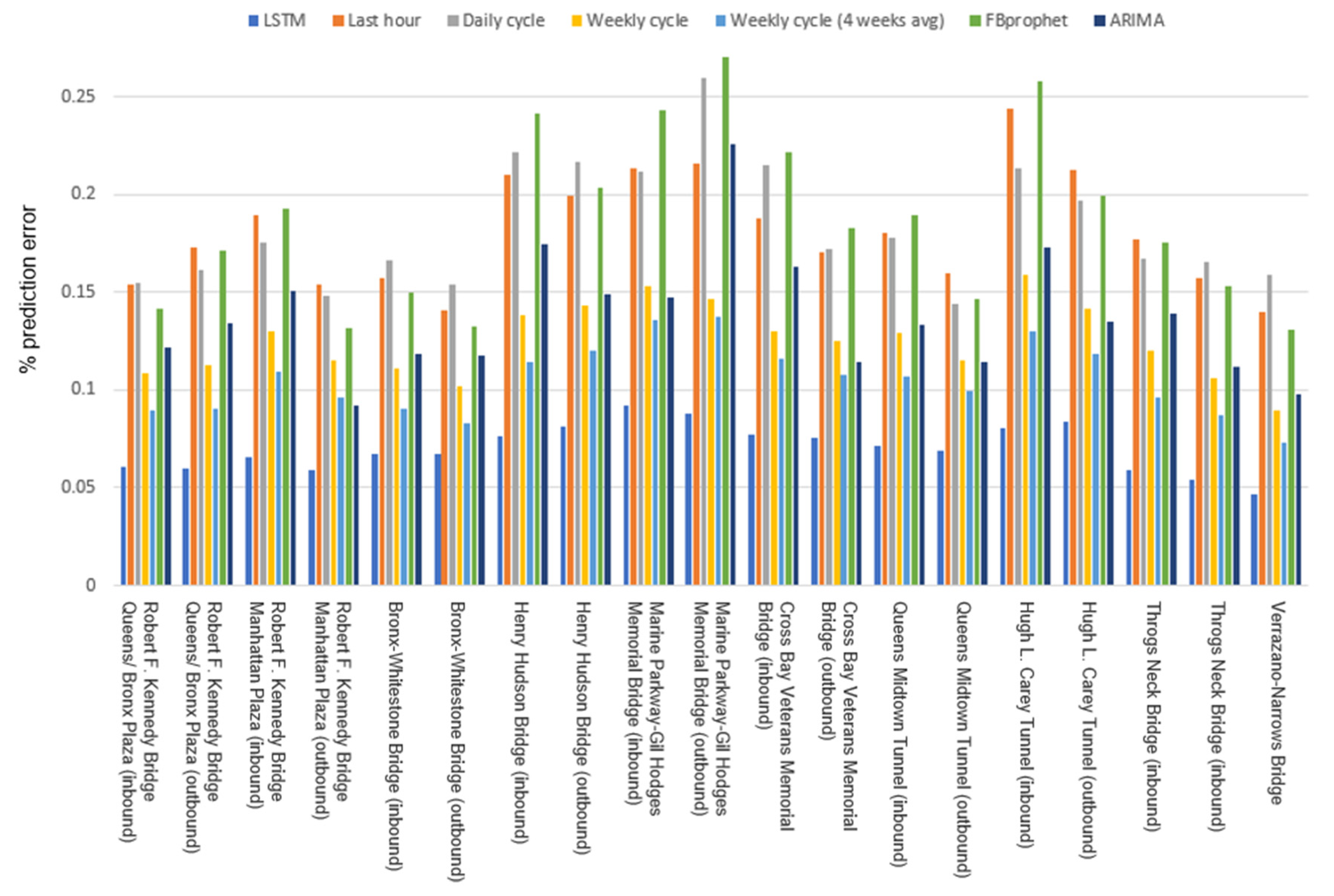
Figure 8 enriches the information, after normalizing by the actual local number of recorded vehicles, presenting the results in terms of percentage of predicted volume error, with respect to the real volume. The LSTM outcomes are reported to range between 4% and 9% of prediction error.
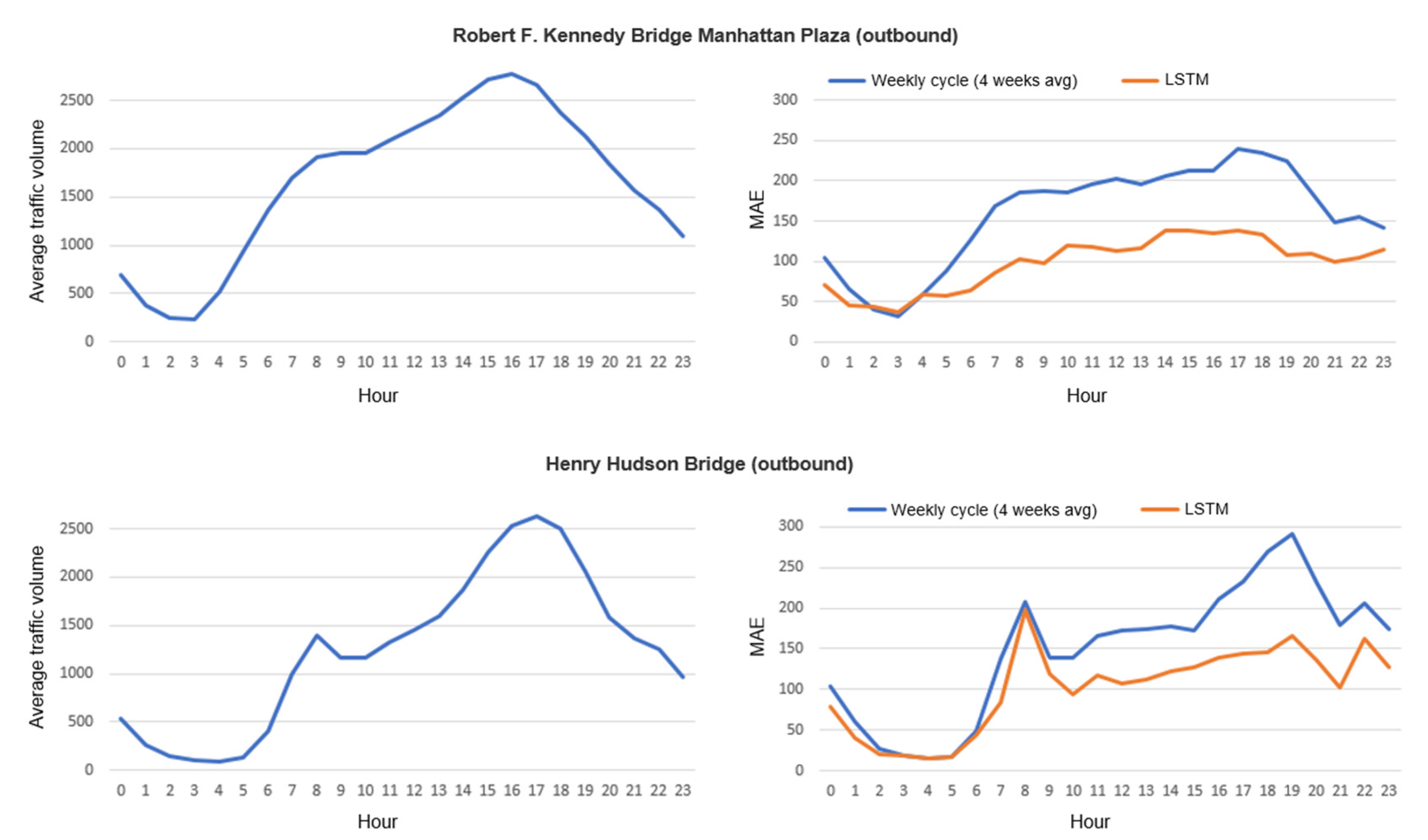
To have a deeper insight into single reference traffic flows, a further analysis may take into account the time variable. It is worth noticing, however, that different flows imply different characteristic behaviors, and different traffic volume variations over time. To acknowledge the presence of various series’ profiles, we report the average daily traffic pattern of two exemplifying reference locations in
Figure 9. The volume variation is depicted together with the overall predictability trend over time, disclosing the forecasting variability over the 24 h. Comparing our model with the best baseline reveals distinctive performance outlines in terms of average hourly prediction error; the maximum improvement is particularly registered during the late afternoon hours.
4. Discussion and Conclusions
The paper proposed a deep neural network approach for predicting traffic volumes, distributed over multiple reference locations across the city. We particularly focused on movements between urban regions, targeting crowded crossing points between contiguous neighborhoods. The task assumed the trait of a short-term forecasting process in a distributed geographic context, grounding its implementation in a sequential modeling perspective. The process relied on a recurrent LSTM-based network model, set up as a multi-target regression problem, involving location-specific sequences of vehicle counts unfolding in a fixed time step. The collection of all reference locations’ input series were concatenated on the time axis, defining each input step as a multi-dimensional vector containing the current distributed amounts of vehicles across the neighborhood connections under study. The prediction outcome, following the same principle, was the product of a multi-target dense layer outputting the time-stamped vector of the expected vehicle distribution across the totality of reference locations. Our case study involved a real-world dataset in New York City, assessing the feasibility of predicting the number of vehicles moving through each of the MTA bridges and tunnels. The scope was therefore enclosed in a short-term distributed traffic volume estimation process, in the context of real-time decision-making strategies and urban management services.
The presented methodology was proposed as an effective solution for capturing rapid variations and abrupt changes beyond the general trends, essential aspect for a proper short-term traffic prediction. Compared to a variety of baselines embodying particular characteristics of the series (steady behaviors and repetitive cycles), our approach reported a superior performance, effect of a significant capability of modeling sequential characteristics of traffic evolution over time in correspondence of multiple distinctive locations. Besides the baselines’ evidence of a prominent weekly-based recurrent cycle, the substantially better results of the deep learning model presumed a presence of more sophisticated inherent patterns in the series, which, when properly mined, revealed information on future traffic changes as a result of more complex properties than a pure cyclical repetitiveness. Contrary to regressive statistical methods, which fit the general trend but were not able to catch sudden variations, our model better identified quick time evolutions of traffic distribution for anticipating short-term rapid leaps in the future.
The experimental results reported outperforming measures over all comparison approaches with respect to each of the 19 selected reference traffic flows in the city, revealing a widespread effectiveness on the whole territory, regardless of geographic locations and local traffic volumes. This indicates a general performance stability, demonstrating the feasibility of collectively modeling a variety of different location-specific characteristic patterns and different traffic profiles over time.
From a practical utilization perspective, it is worth noticing some implicit advantages and facilitations, especially regarding the deployment phase. The proposed approach was designed for processing the collection of reference locations together within one single global training procedure, in contrast to traditional statistical models requiring a separate fit for each different flow. The prediction outcome relies on an instant automatic one-step inference of distributed numbers of vehicles at each time update, releasing the output values of all locations together in a single forecasting block. Furthermore, the neural network does not require a refit for each prediction update, but only a periodical retraining is suggested, depending on the performance degrade caused by evolving behaviors in time.
This work is inserted in the wide field of smart city research [
52], on the side of predictive analytics for advanced decision-making and user-oriented services, leveraging deep learning-based artificial intelligence advancements within a purely data-driven perspective. The broad objective refers to the traffic monitoring and control in an urban environment, implying a variety of applications related to future traffic volume estimations. A straightforward direction leads to predictions of bottlenecks and congestions, enabling real-time urban strategies by local organizations, including warning information messages to drivers about the level of expected traffic distribution in the next hour. Another subject of interest focuses on exploratory studies of inter-neighborhood motion characteristics, portraying a future depiction of human mobility across the city by forecasting entry and exit flows within urban areas; local crowding estimates can be derived from the number of vehicles entering and leaving the city or moving between specific neighborhoods, leading to designing appropriate preventive strategies. Reliable predictions on the spatial distribution of people are important for various tasks, ranging from supply adjustment of location-based services to real-time crowd control related management and countermeasures.
Several further extensions can be identified, subjecting the methodology to specifically targeted modifications accomplishing a wider spectrum of contents. A possible research motive may focus on adapting the model for providing a prediction output that extends over multiple steps in the future, namely forecasting multiple hours ahead and assessing the performance horizon identifying the maximum point in time that still guarantees an advantage over baselines. A further evolution may concern the possibility of handling additional input information (e.g., event-specific instances, weather and environmental factors) within the model architecture, quantifying potential improvements originating from a mixture of contributions; for a widest possible generalization, we indeed leveraged only historical time series, not resorting to any additional information. More generally, similar variants of the proposed methodology can be applied to spatial-temporal phenomena of a different nature, still leveraging geographically-distributed sequential measurements characterized by rapid variations and abrupt location-specific patterns. Finally, following the recent expanding success of deep learning methodologies in a variety of research domains involving sequential processing tasks (e.g., [
53,
54]), focused improvements to the current architecture can be further explored, aiming to enhance the present achievements.
In conclusion, the proposed multi-target LSTM neural network-based model was demonstrated to promisingly handle multiple traffic series belonging to spatially-related reference points, arranging a collective processing of multiple input sequences into corresponding multiple forecasted output values. Representative of an effective application of deep learning on human mobility analysis, the paper contributes to extending a purely data-driven perspective on vehicle number forecasting, tackling a geographically-distributed sequential problem by means of deep neural networks, to aim for an improved quality of urban management and organization.


