Abstract
In the paper, we consider a multi-server retrial queueing system with setup time which is motivated by applications in power-saving data centers with the ON-OFF policy, where an idle server is immediately turned off and an off server is set up upon arrival of a customer. Customers that find all the servers busy join the orbit and retry for service after an exponentially distributed time. For this model, we derive the stability condition which depends on the setup time and turns out to be more strict than that of the corresponding model with an infinite buffer which is independent of the setup time. We propose asymptotic methods to analyze the system under the condition that the delay in the orbit is extremely long. We show that the scaled-number of customers in the orbit converges to a diffusion process. Using this diffusion limit, we obtain approximations for the steady-state probability distribution of the number of busy servers and that of the number of customers in the orbit. We verify the accuracy of the approximations by simulations and numerical analysis. Numerical results show that the retrial system under the limiting condition consumes more energy than that with an infinite buffer in front of the servers.
1. Introduction
Presently, cloud computing is used by many companies and individuals. In our everyday business, we use many kinds of sharing services such as Dropbox, Slack, Overleaf, etc. which are based on cloud computing. Cloud computing is even more important under the current situation where social distancing is encouraged to combat COVID-19, leading to remote work for a large portion of our society. Cloud computing is supported by data centers in which a huge number of servers are available. These servers consume a huge amount of energy and thus saving-energy is crucial in management of data centers and cloud computing. Since user traffic has peak-on and peak-off nature, it is desired that more server resource is allocated in peak-on period and less resource is allocated in peak-off period. Furthermore, because user traffic stochastically varies, we need control policies that add more resources when the workload is large and release resources when the workload is small. The same mechanism is also observed in 5G networks with network functions virtualization (NFV) [1,2]. Motivated by these situations, many power-saving mechanisms were proposed [3,4,5].
One of the most natural mechanisms is the ON-OFF policy which turns OFF a server once it has no job to handle and turns on an OFF server again once a job arrives. However, an OFF server cannot be active immediately to serve the waiting job but needs a setup time, during which the server cannot process the job but consumes energy. Queues with setup time are appropriate models for these situations. A server is turned off when it has no job to process while it is turned on again when waiting jobs are available. These models are challenging because the underlying Markov chain has a non-homogeneous structure, i.e., the number of setup servers may depend on the number of jobs in the system. Gandhi et al. [4] study this problem and propose analysing the model using a renewal reward approach. Phung-Duc [6] analyzes the same model using a generating function approach and a matrix analytic method. Furthermore, structure of the optimal policy was studied by Maccio and Down [5,7].
Furthermore, from the user point of view, the request might be blocked if a resource is not allocated, i.e., all the servers are busy upon arrival. In practice, in case the request is blocked, a protocol will reconnect after some time. This time is random and depends on the number of retries. In some application, the retrial interval is doubled for two consecutive blockings.
Motivated by the above applications, we consider a multiserver retrial queues with setup time. In this model, the server is switched off immediately once it finishes serving a job and no new job is available. An off server will be switched on upon arrival of a job and the server changes to the setup state. After some setup time, the server becomes active so that it can serves the job. If all servers are occupied (serving a job or in setup), the arriving job is blocked and makes a retrial (joins the orbit) after an exponentially distributed time. A retrial job behaves the same as a fresh one. The model was first proposed and numerically analyzed in [8], where a non-trivial sufficient stability condition was derived. Some analytical results for single server case are obtained in [9]. In this paper, we study the model in depth, in which our focus is not a numerical solution but to obtain analytical solution under a specific regime. We consider the situation where the retrial time interval is relatively long. In such a regime, the number of retrial jobs explodes. However, using a proper scaling, we can obtain the explicit distribution for the number of jobs in the orbit. The explicit solution is then used to approximate the distribution of the number of customers in the orbit and that of the states of the servers.
It should be noted that multiserver retrial queues without setup time whose underlying Markov chain is two-dimensional are already very difficult to obtain an analytical solution [10,11]. This paper combines two challenging features, i.e., setup time and retrial. As a result, our model in this paper is formulated by a three-dimensional Markov chain and thus is even more challenging to obtain analytic results. Thus, we consider the system under the slow retrial asymptotic regime.
The slow retrial asymptotic regime was studied by Cohen [12], where the first order asymptotic (a law of large number) for multiserver retrial queue without setup time was obtained in the stationary regime. This result is extended in our paper to the model with setup time in non-stationary regime. Our result states that the scaled number of jobs in the orbit converges to a deterministic process which is characterized by an ordinary differential equation (ODE). Furthermore, we study the second order asymptotics, where the scaled number of jobs in the orbit weakly converges to a diffusion process. The limiting results are then used to obtain the approximation of performance measures. As related works, the second order asymptotic result for multiserver retrial queue without setup was derived in [13] (pp. 55–59). Some recent development of asymptotic analysis of retrial queues can be found in [14,15,16]. Furthermore, we refer to the books [13,17] for basic results of retrial queueing systems. Difussion limits for queueing models have been extensively studied [18,19,20,21,22,23,24]. The methodological difference is that we are based on characteristic function while [18,19,20,21,22,23,24] are based on sample path equations or other techniques.
The rest of our paper is organized as follows. Mathematical description of the problem is presented in Section 2. In Section 3, we obtain main equations for the problem solution. The first stage of the asymptotic analysis is made in Section 4, where we derive function which will be used for further diffusion analysis. Based on the results of the first stage, we obtain the condition for the existence of the steady-state regime for our model in Section 5. The second stage of the asymptotic analysis is made in Section 6, where we derive function which is used together with for the asymptotic diffusion analysis in Section 7. Using obtained continuous distributions, we build approximations for discrete distributions under study in Section 8. In Section 9, we analyze applicability areas of obtained approximations using numerical methods and simulation. Concluding remarks are presented in Section 10.
2. Mathematical Model
We consider a multi-server retrial queue with Poisson arrivals with intensity , infinite-capacity orbit and N servers. On the arrival of a customer, if all servers are busy, the customer goes to the orbit where he or she stays for a random time exponentially distributed with parameter (mean ) and then tries to get a service again. If there is a free server, the customer occupies it. Each server serves a customer in two phases: the first one is a setup time which is exponentially distributed with parameter and the second one is a real service which is exponentially distributed with parameter . After the service completed at the second phase, the customer leaves the system.
The service in the system has a specific feature: when one customer completes its service at the second phase and make its server free, and if we have another customer which is served at the first phase at another server, this customer (which was served at the first phase) immediately goes to the server that just becomes free and starts its service at the second phase. Therefore, its total time of servicing becomes less.
Let us denote:
- is the number of servers that are working at the first phase at the instant t;
- is the number of servers that are working at the second phase at the instant t;
- is the number of customers in the orbit at the instant t;
- is the joint probability distribution of the stochastic process .
The goal of the study is to obtain the probability distribution for the process in the steady-state regime. The problem is solved using the method of asymptotic diffusion analysis [16,25] under an asymptotic condition of long delay in the orbit: (mean retrial interval ).
3. Main Equations
Because the process is a three-dimensional Markov chain, we can write the following equalities. For :
For :
For :
We derive the following system of differential balance equations from here. For :
For :
For :
Denoting and using partial characteristic functions
we obtain the following system of differential equations.
For :
For :
For :
Let us use linear finite difference operators , , , to rewrite the system (1)–(3) in the following compact form:
Here is top-left triangle matrix with entries equal to for indices , , and equal to zero for other numbers . Operators in (4) are defined as follows:
Let us denote the summing operator for indices by , the summing operator for indices by , and the total summing operator by . Then Equation (9) together with (4) may be rewritten in the form
This system of equations is the main for the study of the current paper. We will solve it using the method of asymptotic diffusion analysis [16,25] in the next sections.
4. First Stage of Asymptotic Analysis
Let us find the solution of system (10) using the method of asymptotic analysis [16,25] under asymptotic condition of long delay in the orbit: . To do this, let us make the following substitutions:
Then we obtain the following system:
We can prove the following statement.
Theorem 1.
Under the asymptotic condition , the following equality holds.
Here the scalar function is a solution of ordinary differential equation
where is a left-top triangle matrix which is a solution of homogeneous linear system
and satisfies the normalization condition
Proof.
Denoting and making asymptotic transition in (11), we derive
We find the solution of this system in the form
where is a top-left triangle matrix with non-zero entries for , and is a scalar function which has a meaning of asymptotic (while ) value of the normalized number of customers in the orbit . Entries have a meaning of asymptotic (while ) probabilities that servers are working at the first phase and servers are working at the second phase. Substituting (17) into (16), we obtain equalities (14) and (13). Because entries of matrix are probabilities, they satisfy (15). Since the scalar function is an asymptotic value of the normalized number of customers in the orbit , equality (12) is true. The theorem is proved. □
Probability distribution is a solution of system of Equation (14) whose coefficients depend on x, then is a matrix function: . Due to this, we can rewrite (13) as the following expression:
which determines the function . This function is very important for the study due to the following two reasons. The first one is that we showed that . Therefore, function characterizes dynamic properties of the process . The second reason is that will be used in Section 7 as a drift coefficient for the diffusion process which determines the asymptotic number of customers in the orbit.
Remark 1.
For (the mean retrial time ), the number of customers in the orbit explosively increases, Theorem 1 shows that converges to a deterministic process independent of σ and thus has the same order as . Theorem 1 can be interpreted as the law of large numbers.
5. Existence of Steady-State Regime
Considering function which is determined as (18), let us derive a condition of steady-state regime existence.
Due to (18), and values of the process are growing in the neighborhood of point . If for all x, then steady-state regime does not exist in the considered retrial queue. The inequality is the necessary condition for the existence of the steady-state regime.
Let us prove the following statement.
Theorem 2.
Steady-state regime in the considered retrial queue exists if and only if
Proof.
Sufficiency of condition (19) was proved in [8]. Let us prove its necessity. We rewrite (18) in the form:
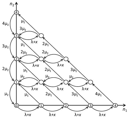
To determine value of , let us find limit properties of probabilities under . Transition intensities for states are depicted in Figure 1 (for simplicity, we draw the graph for partial case of ). In the considered system, we have the following possible transitions:
Figure 1.
Transition for states .
- from state to state with intensity , where is an intensity of arrivals and x is an asymptotic intensity of retrials from orbit,
- from state to state with intensity when one of customers completes service at the first phase and goes to the second one,
- from state to state with intensity for when one of customers completes its service at the second phase and leaves the system but one customer served at the first phase instantly goes to the second phase,
- from state to state with intensity when one of customers completes its service at the second phase and leaves the system.
Using the method cut of graph, we derive equations for probabilities . We can derive them from system of (14) and (15) but it is clearer how they are obtained if using cut of graph. It should be noted that the system of (14) and (15) is equivalent to the system of equations for finding the stationary distribution of the Markov chain with the transition diagram as in Figure 1. This Markov chain represents the M/M/N/N queueing system with setup time with the arrival rate given by .
For diagonal cuts when we can write
Therefore, under the limit condition all the probabilities are equal to zero when . Then due to the normalization requirement, we have
and, so, all non-zero probabilities are located on the diagonal . Moreover, from (21), it follows that all the sums are infinitesimals of order for . For horizontal cuts we can write the following equalities:
Points for lay on diagonals of the graph, therefore, all for are infinitesimals of order . Then all the sums are infinitesimals of order too. Hence, for , the sum and probability have the infinitesimal order of . For , all the sums and probabilities are infinitesimals of order or higher. Therefore, under the limit , only two probabilities and are not equal to zero. Due to the normalization condition, we can write the following:
Solution of this system is as follows:
Let us consider the sum . As we find before, it is an infinitesimal of order . Let us write the equation for the probability :
Here is an infinitesimal of order , hence, the probability , which is multiplied here by x, also, is an infinitesimal of order because only in this case equality (24) is true and sum is an infinitesimal of order . Therefore, for , only one probability has infinitesimal order , all other probabilities have higher infinitesimal order. Let us write equation for the probability as follows:
Taking here the limit , we obtain
Due to (23), we can rewrite it as follows:
Let us come back to the function which determines derivative of the process under asymptotic condition . Let us find limit of the function from (20) under condition . Due to (22) and (25), we can write
Because is necessary for the existence of steady-state regime, the condition (19) is true. The theorem is proved. □
Remark 2.
In [6], the M/M/N/Setup model with infinite buffer is analyzed and the stability condition is given . Theorem 2 shows that the stability condition for the corresponding retrial model is more strict than that of the infinite buffer counterpart.
6. Second Stage of Asymptotic Analysis
In Section 4, we made the first stage of the asymptotic analysis and, similar to the law of large numbers, we obtain equality (12) which determines the convergence of characteristic function of the process to the deterministic function under condition . Now, let us perform the second stage of the asymptotic analysis to obtain more detailed parameters of the convergence.
Let us make the following substitution in system (10)
We obtain
Substitution (26) is made to go to a centered process for : the function is a matrix characteristic function of the centered process , where function have been obtained at the first stage of the asymptotic analysis in Section 4.
We can prove the following statement.
Theorem 3.
Let be an asymptotic (as ) characteristic function of normalized and centered process :
Then it satisfies the equation
where function is determined by (18), has the form
and top-left triangle matrix is a particular solution of the system of equations
and satisfies additional condition
Proof.
We rewrite the first equation of (29) with precision up to infinitesimals of order :
and let us write its solution in the form of expansion:
where is some matrix function whose expression we will obtain later. Substituting (36) into (35), we obtain
Taking into account (14) and dividing by , under the asymptotic condition , we obtain the following equation for the matrix function :
Applying the superposition principle, we can write a solution of this equation in the form
Differentiating (14) by x, we obtain equation
which coincides with (40). Therefore, its solution may be presented in the form
Notice that an additional condition is true due to the normalization condition. Because matrix function is a particular solution of non-homogeneous system (39), we choose an additional equation for it in the form (34) so that is uniquely defined. Let us write the second equation of system (29) with the precision up to :
Substituting (36) here, we obtain
Taking into account (13), combining similar terms, dividing by and taking the limit , we derive
Substituting (38) here and taking into account that , , and , we obtain the following equation:
This is the coefficient in the first term in the right part of (42). As for the coefficient in the second term, we denote as :
Remark 3.
Theorem 3 shows that converges to a diffusion process. This can be regarded as a central limit theorem for the process , where the mean is and the variance is .
7. Method of Asymptotic Diffusion Analysis
In this section, we consider an implementation of the method of asymptotic diffusion analysis for obtaining probability distribution of the process of the number of customers in the orbit under asymptotic condition in considered retrial queue. In what follows, we use y and interchangeably.
Let us make the following inverse Fourier transform in (31):
We obtain the equation
Here is a limit for the normalized and centered process ; is its characteristic function and is its probability density function (p.d.f.).
Equation (44) is the Fokker – Planck equation for p.d.f. , therefore, the process is a diffusion process with a drift coefficient equal to and a diffusion coefficient equal to .
Diffusion process is a solution of the stochastic differential equation
where is the Wiener process. This equation is difficult to solve directly.
We rewrite the ordinary differential Equation (13) in the form:
Consider the following stochastic process:
where as in the previous section. It is easy to confirm that the process is the limit of the normalized process under condition . Thus, has a more direct relation with which is the quantity of interest.
We derive a stochastic differential equation for .
Let us rewrite coefficients in this equality in the form using the first order Taylor series expansion with respect to .
So, we can rewrite the equality with precision up to as follows:
Due to , we can write the equation
which is a stochastic differential equation and its solution is a diffusion process with drift coefficient and diffusion coefficient .
Stationary p.d.f. of the process is a solution of the Fokker–Planck equation
We find a solution of this differential equation in the form.
The general solution for this differential equation is given in the form.
where C is an arbitrary constant. Because, we are looking for a solution which is a probability density function with support in , we choose C as follows.
Therefore, we found asymptotic probability density function of the normalized number of customers in the orbit in the steady state, i.e., as and then . In the next section, we further use it to build a discrete distribution of the number of customers in the orbit.
8. Approximations of Steady-State Distributions
The goal of the work is to find enough precise approximations for discrete probability distribution of the number of servers working in the first and in the second phases and for probability distribution of the number of customers in the orbit in steady-state regime of considered multi-server retrial queue with setup time.
Two-dimensional probability distribution can be approximated by entries of the top-left triangle matrix if we choose appropriate value x of function which is determined by the differential equation . To do this, we choose where is a positive root of the equation
For such value of x we have that means the steady-state regime.
Algorithm for constructing of the approximations and for and is as follows. Here and are the probabilities that the number of busy servers (in both phases) is n.
1. Let us rewrite Equation (14) for entries of the matrix :
and let us find a solution of the system which satisfies the normalization requirement for given and .
2. From equality (13), we derive
3. Using numerical methods, we find a solution of the equation
4. Substituting into , we obtain approximation of two-dimensional probability distribution of the number of servers working in the first and in the second phases of service.
5. Using expression
we find approximation of the probability distribution of the number of busy servers in the considered retrial queue.
To find an approximation for discrete steady-state probability distribution of the number of customers in the orbit, we apply p.d.f. of continuous limit process normalized by . To do this, we apply expression (48) and find values of the following function:
We obtain an approximation for the distribution in the form
It should be noted that this approximation is not unique and we might choose other alternative distribution also [26].
Algorithm of constructing of the approximation is as follows.
Then we find solution of this system which satisfies additional requirement for given and .
2. From (32), we can write
Here , therefore, we can write function in the form
3. We substitute obtained functions and into (52) to calculate values .
4. Applying (53), we obtain probability distribution which approximates the goal distribution for small values of .
9. Applicability Area of Obtained Results
To estimate precision and applicability area of obtained approximations, we compare the results with empiric probabilities obtained on the base of simulation results. For numerical estimation of the error, we traditionally use Kolmogorov distance
where and are discrete distributions that should be compared. In our case, one of them is approximation (53) and another one is an empiric distribution of the number of customers in the orbit obtained from simulation results.
We use
as a precision criterion for the approximation to be applicable. To avoid simulation error influence, we choose such sample sizes in the simulation experiments to empiric distributions have error (to estimate it, we use comparisons between several simulation results). You may choose any level of the error in the form of the Kolmogorov distance. Due to the definition of the Kolmogorov distance, the value 0.05 may be interpreted as a 5% error and this fact has no other meaning.
For simulation experiments, the following parameters of the retrial queue with setup time were chosen: the number of servers , setup time distribution parameter , main service distribution parameter . Intensity of arrivals were chosen to satisfy steady-state existence requirement (19). Therefore, if we denote the system load parameter by , then we can choose value of as follows:
This can be rewritten as
representing the traffic intensity of our system.
We will vary parameters and such that (55) is satisfied. Results of such analysis for various values of parameters and are presented in Table 1. We highlight by boldface font values that satisfy condition (55). Therefore, we can conclude that obtained approximation (53) becomes more precise when system load parameter grows and delay in the orbit increases ( becomes less). For values and for values it becomes applicable in a wide range.

Table 1.
Values of Kolmogorov distance () of approximation distribution given by (53) and its exact one (by simulation) for various values of (retrial rate) and (traffic intensity). The cases with are in boldface.
Distributions of the number of customers in the orbit obtained by simulation experiments and by the approximation for are shown in Figure 2. As one can see, these distributions are very close to each other and especially for the cases () where , and this fact proves the high accuracy of the obtained approximation. Just for large values of , we have a jump at the starting point in real distribution which we cannot approximate properly.
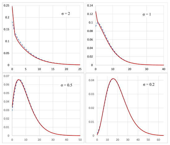
Figure 2.
Comparisons of the approximation (dashed line) and the simulation results (solid line) obtained for the probability distribution of the number of customers in the orbit for and various values of .
An important observation is that the approximation becomes more accurate as the traffic intensity increases. This is because, we approximate the scaled number of customers in the orbit by a truncated distribution of the one (stationary distribution of the diffusion process) which might have negative support. When the traffic intensity, the mass for negative part is small and thus this approximation is appropriate.
Results on errors in mean and variance for these distributions are shown in Table 2.
Table 2.
Errors in mean and variance of approximation distribution given by (53) for and various values of .
In Figure 3, we compare the mean power consumption of our model in the limitting regime (denoted by Asymptotic) with that of the buffered model [6], i.e., instead of retrial, blocked customers join the buffer in front of the servers (). Figure 3 shows the total power consumption by setup servers (phase 1) and active servers (phase 2) against the arrival rate . We assume that both the setup server and the active one consume an energy unit per unit time. Thus, the power consumption is equal to the mean of the sum of the number of setup servers and that of active ones. The mean number of setup servers and that of active ones in the limit regime is calculated using the distribution and is given by . For a reference, we also plot the power consumption of the ON-IDLE model (M/M/c queue), where the mean number of active servers and that of idle servers are given by and , respectively. Here we assume that power concumption of an idle server is of 60% that of an active one. As a result, power consmption for hte ON-IDLE model is simply given by . Fixed parameters are given by for both models. We observe that the power consumption of the asymptotic regime is larger than that of the buffered model. This is intuitive because in the buffered model, once a server completes a service (phase 2), a waiting customer can immediately occupy the server without setup (phase 1). Furthermore, ON-OFF models are more power-saving than the ON-IDLE model when the arrival rate is relatively small, and the opposite trend is observed when the arrival rate is large enough.
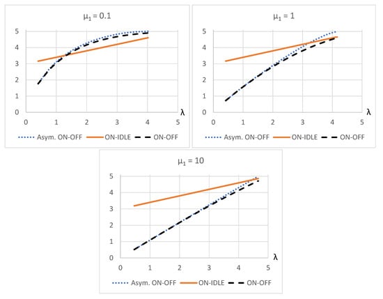
Figure 3.
Power consumption against the arrival rate .
10. Conclusions
In the paper, we considered a multiserver retrial queue with setup time. Using methods of asymptotic analysis under the condition of long delay in the orbit, we derived necessary condition for the existence of the steady-state regime. Using the method of asymptotic diffusion analysis, we obtained diffusion process whose probability density function is used an approximation for the probability distribution of the number of customers in the orbit. Using simulations and numerical experiments, we showed that the approximation is good for a wide enough range of parameters. Further studies may be made for more complex models with setup time, e.g., models with impatient customers and/or with outgoing calls. The asymptotic regime where the number of servers tends to infinity [18,27] might also be worth for investigation. In our paper, although we proved that the scaled version of the number of customers in the orbit converges to a diffusion process which has a stationary distribution. In the future work, we plan to give a rigorous proof of the convergence of the stationary scaled number of customers in the orbit to the stationary distribution of the diffusion process.
Author Contributions
Conceptualization, A.N., T.P.-D.; formal analysis, A.M., T.P.-D.; investigation, A.M., A.N., S.P., T.P.-D.; methodology, A.N.; software, A.M.; writing–original draft, S.P.; writing–review & editing, A.M., T.P.-D. All authors have read and agreed to the published version of the manuscript.
Funding
The third author T.P. was supported in part by JSPS Kakenhi No. 18K18006.
Conflicts of Interest
The authors declare no conflict of interest.
References
- Ren, Y.; Phung-Duc, T.; Chen, J.C.; Yu, Z.W. Dynamic auto scaling algorithm (dasa) for 5g mobile networks. In Proceedings of the 2016 IEEE Global Communications Conference (GLOBECOM), Washington, DC, USA, 4–8 December 2016; pp. 1–6. [Google Scholar]
- Phung-Duc, T.; Ren, Y.; Chen, J.C.; Yu, Z.W. Design and analysis of deadline and budget constrained autoscaling (DBCA) algorithm for 5G mobile networks. In Proceedings of the 2016 IEEE international conference on cloud computing technology and science (CloudCom), Luxembourg, 12–15 December 2016; pp. 94–101. [Google Scholar]
- Gandhi, A.; Harchol-Balter, M.; Adan, I. Server farms with setup costs. Perform. Eval. 2010, 67, 1123–1138. [Google Scholar] [CrossRef]
- Gandhi, A.; Doroudi, S.; Harchol-Balter, M.; Scheller-Wolf, A. Exact analysis of the M/M/k/setup class of Markov chains via recursive renewal reward. ACM Sigmetrics Perform. Eval. Rev. 2013, 41, 153–166. [Google Scholar] [CrossRef]
- Maccio, V.J.; Down, D.G. Structural properties and exact analysis of energy-aware multiserver queueing systems with setup times. Perform. Eval. 2018, 121, 48–66. [Google Scholar] [CrossRef]
- Phung-Duc, T. Exact solutions for M/M/c/setup queues. Telecommun. Syst. 2017, 64, 309–324. [Google Scholar] [CrossRef]
- Maccio, V.J.; Down, D.G. On optimal control for energy-aware queueing systems. In Proceedings of the 2015 27th International Teletraffic Congress, Ghent, Belgium, 8–10 September 2015; pp. 98–106. [Google Scholar]
- Phung-Duc, T.; Kawanishi, K. Multiserver retrial queue with setup time and its application to data centers. J. Ind. Manag. Optim. 2019, 15, 15–35. [Google Scholar] [CrossRef]
- Phung-Duc, T. Single server retrial queues with setup time. J. Ind. Manag. Optim. 2017, 13, 1329–1345. [Google Scholar] [CrossRef]
- Phung-Duc, T.; Masuyama, H.; Kasahara, S.; Takahashi, Y. M/M/3/3 and M/M/4/4 retrial queues. J. Ind. Manag. Optim. 2009, 5, 431–451. [Google Scholar] [CrossRef]
- Phung-Duc, T.; Masuyama, H.; Kasahara, S.; Takahashi, Y. State-dependent M/M/c/c+ r retrial queues with Bernoulli abandonment. J. Ind. Manag. Optim. 2010, 6, 517–540. [Google Scholar] [CrossRef]
- Cohen, J.W. Basic problems of telephone traffic theory and the influence of repeated calls. Philips Telecommun. Rev. 1957, 18, 49–100. [Google Scholar]
- Falin, G.I.; Templeton, J.G.C. Retrial Queues; Chapman & Hall: London, UK, 1997. [Google Scholar]
- Danilyuk, E.Y.; Moiseeva, S.P.; Sztrik, J. Asymptotic Analysis of Retrial Queueing System M/M/1 with Impatient Customers, Collisions and Unreliable Server. J. Sib. Fed. Univ. Math. Phys. 2020, 13, 218–230. [Google Scholar] [CrossRef]
- Fedorova, E.; Nazarov, A.; Moiseev, A. Asymptotic Analysis Methods for Multi-Server Retrial Queueing Systems. In Applied Probability and Stochastic Processes; Springer: Singapore, 2020; pp. 159–177. [Google Scholar]
- Moiseev, A.; Nazarov, N.; Paul, S. Asymptotic Diffusion Analysis of Multi-Server Retrial Queue with Hyper-Exponential Service. Mathematics 2020, 8, 531. [Google Scholar] [CrossRef]
- Artalejo, J.R.; Gomez-Corral, A. Retrial Queueing Systems; Springer: Berlin/Heidelberg, Germany, 2008. [Google Scholar]
- Halfin, S.; Whitt, W. Heavy-traffic limits for queues with many exponential servers. Oper. Res. 1981, 29, 567–588. [Google Scholar] [CrossRef]
- Mandelbaum, A.; Massey, W.A.; Reiman, M.I. Strong approximations for Markovian service networks. Queueing Syst. 1998, 30, 149–201. [Google Scholar] [CrossRef]
- Robert, P. Stochastic Networks and Queues; Springer Science & Business Media: Berlin/Heidelberg, Germany, 2013; Volume 52. [Google Scholar]
- Whitt, W. On the heavy-traffic limit theorem for GI/G/∞ queues. Adv. Appl. Probab. 1982, 14, 171–190. [Google Scholar] [CrossRef]
- Whitt, W. Stochastic-Process Limits: An Introduction to Stochastic-Process Limits and Their Application to Queues; Springer Science & Business Media: Berlin/Heidelberg, Germany, 2002. [Google Scholar]
- Whitt, W. Efficiency-driven heavy-traffic approximations for many-server queues with abandonments. Manag. Sci. 2004, 50, 1449–1461. [Google Scholar] [CrossRef]
- Pender, J.; Phung-Duc, T. A law of large numbers for M/M/c/delayoff-setup queues with nonstationary arrivals. In Analytical and Stochastic Modelling Techniques and Applications; LNCS 9845; Springer: Cham, Switzerland, 2016; pp. 253–268. [Google Scholar]
- Nazarov, A.; Phung-Duc, T.; Paul, S.; Lizura, O. Asymptotic-Diffusion Analysis for Retrial Queue with Batch Poisson Input and Multiple Types of Outgoing Calls. In International Conference on Distributed Computer and Communication Networks; LNCS 11965; Springer: Cham, Switzerland, 2019; pp. 207–222. [Google Scholar]
- Jantschi, L. A Test Detecting the Outliers for Continuous Distributions Based on the Cumulative Distribution Function of the Data Being Tested. Symmetry 2019, 11, 835. [Google Scholar] [CrossRef]
- Maccio, V.J.; Down, D.G. Asymptotic performance of an energy-aware G/G/C queue with general setup times. Queueing Model. Service Manag. 2020, 3, 111–135. [Google Scholar]
Publisher’s Note: MDPI stays neutral with regard to jurisdictional claims in published maps and institutional affiliations. |
© 2020 by the authors. Licensee MDPI, Basel, Switzerland. This article is an open access article distributed under the terms and conditions of the Creative Commons Attribution (CC BY) license (http://creativecommons.org/licenses/by/4.0/).