Predicting Benzene Concentration Using Machine Learning and Time Series Algorithms

Abstract

Benzene is a pollutant which is very harmful to our health, so models are necessary to predict its concentration and relationship with other air pollutants. The data collected by eight stations in Madrid (Spain) over nine years were analyzed using the following regression-based machine learning models: multivariate linear regression (MLR), multivariate adaptive regression splines (MARS), multilayer perceptron neural network (MLP), support vector machines (SVM), autoregressive integrated moving-average (ARIMA) and vector autoregressive moving-average (VARMA) models. Benzene concentration predictions were made from the concentration of four environmental pollutants: nitrogen dioxide (NO₂), nitrogen oxides (NO_x), particulate matter (PM₁₀) and toluene (C₇H₈), and the performance measures of the model were studied from the proposed models. In general, regression-based machine learning models are more effective at predicting than time series models.

1. Introduction

Volatile organic compounds (VOCs) are compounds with very high volatility which are in a gaseous state under normal circumstances. They include a variety of chemical species among which are benzene, toluene, ethylbenzene and xylene [1] and are known as BETX, all of them are air pollutants, along with other compounds such us SO₂, NO₂, NO_x, PM₁₀, PM_2.5 or CO [2].

Benzene is a hydrocarbon with a ring structure made up of six carbon atoms. It is one of the products that is most used as a raw material in industrial processes in the organic chemical industry. Its usual state is liquid, highly flammable, and colorless, although it does have a very characteristic odor and very high toxicity [3].

Benzene has been used in the manufacture of several chemical products like styrene, phenols, in nylon and synthetic fibers, maleic anhydride, pharmaceuticals, detergents and dyes and explosives. It has also been used in fuel, where it is added as a lead substitute, chemical reagent and extraction agent for other chemical compounds [3]. Derivates of benzene are used primarily as solvents and diluents in the manufacture of perfumes and in intermediates in the production of dyes, although the most important industrial use is as solvents and paint thinners [4,5].

Benzene has been banned as a component of products intended for domestic use and, in many countries, it has also been prohibited as a solvent and as a component of dry-cleaning liquids [4].

Natural sources of benzene include emissions from volcanoes and forest fires [6]. On the other hand, road traffic is an important source of emissions of VOCs, such as benzene, and other compounds that mainly come from vehicle exhausts and are generated during the incomplete combustion of fuels [7].

A study [8] has reported that there is a big discrepancy between the values obtained in measurements of industrial environments compared to the homogeneous values obtained in urban areas.

The main source of benzene exposure is tobacco smoke and other outdoor sources like automobile exhaust emissions [5], combustion processes and industrial chemical vapors [8]. Indoor sources include building materials, detergents, glues, furniture varnish and products such as solvents and paints from kitchens, attached garages and fuels for housing. The concentration of benzene indoors is generally higher than it is outdoors. It is affected by weather conditions and by the type of ventilation [3,5]. However, personal exposure concentrations of benzene in and around gas stations is considerably higher than indoor and ambient concentrations [9].

Recent studies [10] indicate that, while the limits of indoor concentration have been increasingly restrictive and the sources of interior emissions have been progressively reduced, outdoor benzene has become a significant, and even in many cases dominant, contributor to indoor concentration.

Air pollution is associated with adverse health effects such as respiratory and cardiovascular diseases, cancer and even death [11]. In 2017, environmental contamination contributed to almost 5 million premature deaths in the world [12]. More than 90% of the world’s population lives in areas where the WHO-established guidelines for the quality of healthy air are exceeded and about half, a total of 3.6 billion, was exposed to contamination in the home. Air pollution is related to premature deaths from ischemic heart disease (16%), chronic obstructive pulmonary disease (41%) and lung cancer (19%).

The sources of entry of benzene into the human body are the lungs, the digestive tract and the skin [5] although population exposure is mainly produced through the inhalation of air containing benzene [8].

Several factors influence benzene exposure, including mainly concentration, duration of exposure, contact pathway and also the presence of other chemical substances, as well as the characteristics and habits of people [5].

A long or repeated exposure to benzene can affect the central nervous system and the immune system. It can also affect the bone marrow, and this can cause anemia and different types of leukemia. It may also cause inherited genetic damage in human germ cells [4,13].

Benzene has been categorized as being among group I carcinogens by the International Agency for Research on Cancer (IARC). It is considered as a known human carcinogen and no safe level can be recommended [3,14,15].

Sensitive population groups such as the elderly, pregnant women, infants, children and people with previous cardiovascular and respiratory diseases are the most susceptible to poor air quality [16]. Several studies indicate that there is a strong relationship between air pollution and infant mortality [17] and diseases of the infant respiratory system, so that hospital admissions increase significantly when there are pollution peaks. Hospital admissions for other causes also increase when benzene levels and other air pollutants rise [18,19,20].

Epidemiological studies have shown that there is a relationship between exposure to benzene and the development of acute myeloid leukemia [14]. A Swiss pediatric oncology cohort study [21] found an increased risk of leukemia among children whose mothers had been exposed to benzene at work. Studies like [22] also indicate the existence of an increased risk of colon cancer in Nordic countries, while a study in France showed that long-term exposure to outdoor air pollution like benzene, fine particles, sulfur dioxide and nitrogen dioxide is a significant environmental risk factor for mortality [23].

There are different limits established for exposure to benzene. The European Commission has established a concentration limit for benzene of 5 µg/m³ as an annual averaging period in the Directive 2008/50/EC, Directive on environment air quality [24].

Regarding occupational exposure limits [13], TLV-TWA of 0.5 ppm (the threshold limit value considered as the time-weighted average for an 8 h day and 40 weekly hours) and 2.5 ppm as STEL (short-term exposure limit for periods of 15 min that should not be exceeded at any time) have been established.

OSHA regulates benzene levels in the workplace. The maximum amount of benzene in the air must not exceed 1 ppm during an 8 h day, 40 h a week [5] (Directive 97/42/EC, amendment of 90/394/EEC).

Environmental pollution processes are complex and direct measurement is not always possible. In addition, it is difficult to carry out an analysis to discover the source, the propagation and distribution models and to make predictions over time. Therefore, since the reduction of such pollution is an objective of the European Union, it is necessary to find methods that make it possible to model its behavior and predict its evolution.

In the case of pollution concentration modeling, there are two methodologies used in predicting air quality: physical models and models based on statistical data. Physical models are based on chemical dispersion and transport models, in which the input variables are often related to parameters obtained from meteorological observations, such as air temperature, dew point, relative humidity, atmospheric pressure, speed and direction of wind, UV radiation, another group of parameters related to the terrain such as vegetation, local topography, etc. and parameters related to emission sources that represent changes in traffic patterns, industrial activity and the distance to these sources. Statistical machine learning models are based on periodic parameters and these models do not need to understand physical phenomena. Models based on statistical parameters achieve better predictions than models that only used meteorological variables as input [25].

The objective of this study was to predict the concentration of benzene from other pollutants, which were collected by several measurement stations of the Community of Madrid (Spain) every day during the period indicated in

Table 1. Stations.

Station	Code	Name	Latitude (Degree)	Longitude (Degree)	Altitude (m)	Measurement Dates
6	28,079,006	Marañón	40.437567	−3.690759	669	2001–2009
15	28,079,015	Pz Castilla	40.465595	−3.688740	729	2001–2008
22	28,079,022	Pontones	40.406326	−3.712948	618	2001–2005
23	28,079,023	Alcalá final	40.448702	−3.609647	642	2001–2009
25	28,079,025	Sta Eugenia	40.379079	−3.602494	658	2001–2005
26	28,079,026	Embajada	40.459303	−3.580089	611	2005–2010
27	28,079,027	Barajas	40.476931	−3.580018	621	2005–2009
35	28,079,035	Pz Carmen	40.419216	−3.703165	659	2001–2006

for each station, constituting voluminous information that allows their mathematical modeling and statistical learning to obtain an explanation of the dependency among the main pollutants in a geographic area based on the concentrations of other air pollutants in each station, as well as the environmental pollution existing at that time in other stations.

To make this prediction, time series forecasting techniques such as autoregressive moving average vectors (VARMAs), and integrated autoregressive moving average model (ARIMA) were applied and the results compared with those obtained with machine learning methodologies such as artificial neural networks (ANNs), support vector machines (SVMs), multivariate linear regressions (MLRs) and multivariate adaptative regression splines (MARSs).

In existing literature there are several success stories of applying these methodologies as a tool for predicting contamination and dispersion of air pollutants such as SO₂, NO₂, NO_x, PM₁₀, PM_2.5 O₃ or CO.

There are multiple studies of different pollutants to make predictions with ANNs such as [25,26,27,28]. Other models like SVMs have been studied by [29,30,31]. MLRs by [32,33]. Time data series by [34,35,36,37] and MARSs by [38,39].

In many of these articles they analyze different models, compare the results and determine which method makes the best predictions for the pollutants that have been studied [40,41].

A previous study [28] reviewed 139 articles about pollutants examined with ANN models and the results indicate that the most analyzed pollutants are particulate matter (PM₁₀, PM_2.5) in 62% of the articles, 36% nitrogen oxides (NO, NO₂ and NO_x), 31% O₃. SO₂ and CO modeling in 13% and 16% of articles. Almost a third of them include the study of several pollutants, but only one article [42], has studied an ANN model for predicting benzene.

Therefore, models for the prediction of benzene have not yet been developed, and even less so to study the relationship between measurements obtained from other pollutants at stations with benzene. The methods used are data-oriented, so there is no need to make solid chemical-physical assumptions during the modeling process, they have the capacity to handle large amounts of data and are applied in different tasks such as studying the existing relationship between benzene and the rest of pollutants and its prediction.

2. Materials and Methods

2.1. The Database

In this study, data observed from various pollutants was used, along with four predictor variables: nitrogen dioxide (NO₂), nitrogen oxides (NOx), particulate matter with a diameter less than 10 µm (PM₁₀), and toluene (C₇H₈) were selected to perform the benzene (C₆H₆) prediction models.

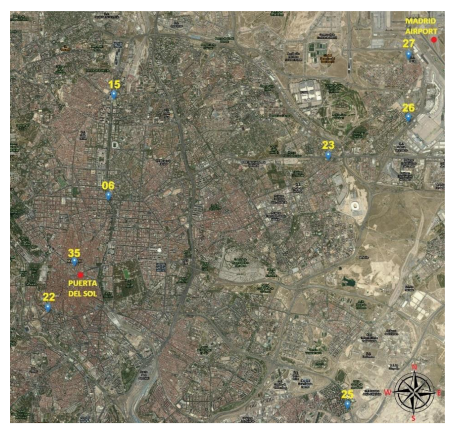
These pollutants were collected by eight remote measurement stations in the Community of Madrid (Spain) every day, with hourly measurements during the periods indicated in Table 1. Figure 1 shows the geographical location of the stations used in this study on the map of Madrid.

Before carrying out the formation phase of the models used, an imputation of the missing data due to breakdowns and maintenance of the stations was carried out, through multiple imputations by chained equations [43].

The mean and standard deviation of the pollutants under study are shown in

Table 2. Mean and standard deviation of pollutants in each station (BEN: benzene, NO₂: nitrogen dioxide, NO_x: nitrogen oxides, PM₁₀: particles with a diameter of 10 micrometres or less and TOL: toluene).

	St 6	St 15	St 22	St 23	St 25	St 26	St 27	St 35
BEN	2.989 (2.789)	2.544 (2.875)	2.544 (3.423)	1.403 (2.4472)	1.818 (2.153)	0.317 (0.395)	0.327 (0.402)	2.116 (1.999)
NO2	79.116 (40.162)	69.170 (31.930)	56.489 (30.572)	59.861 (34.839)	62.005 (35.887)	63.932 (34.562)	40.907 (28.208)	70.052 (32.049)
NOx	186.404 (149.716)	146.949 (107.172)	128.100 (117.860)	113.233 (126.986)	142.531 (135.603)	99.519 (88.431)	68.115 (65.472)	142.569 (120.250)
PM10	39.065 (29.477)	35.9547 (27.948)	32.097 (26.910)	31.747 (28.422)	38.894 (34.107)	26.529 (23.114)	25.127 (22.961)	35.638 (29.355)
TOL	14.331 (14.249)	9.751 (10.184)	10.012 (11.220)	7.408 (10.233)	8.778 (11.519)	2.003 (4.762)	2.130 (3.716)	11.774 (11.274)

.

2.2. Multivariate Linear Regression

Linear regression with several independent variables is known as multivariate or multiple linear regression (MLR), which is a generalization of simple regression when the relationship of a dependent variable designated by $Y$ is represented by the linear combination of the other k independent variables, which are denoted by $X_1,X_2,\dots ,X_k$.

MLR model assumes a relationship of the type $Y={\beta }_0+{\beta }_1{X}_1+{\beta }_2{X}_2+\dots +{\beta }_k{X}_k+\epsilon$, where ${\beta }_0, {\beta }_1, {\beta }_2,\dots ,{\beta }_k$ are (k + 1) parameters called regression coefficients and $\epsilon$ is the stochastic error associated with the regression. Regression parameters $\beta$ are estimated in order to determine the best hyperplane among all of the form $y_t={\widehat{\beta }}_0+{\widehat{\beta }}_1{x}_1+{\widehat{\beta }}_2{x}_2+\dots +{\widehat{\beta }}_k{x}_k$. A set of n observations is available for each of the dependent and independent variables, so the model is as follows [44,45]:

$$Y_j={\widehat{\beta }}_0+{\widehat{\beta }}_1{X}_{1j}+{\widehat{\beta }}_2{X}_{2j}+\dots +{\widehat{\beta }}_k{X}_{kj}+{\epsilon }_j, j=1,2,\dots , n$$

(1)

In order to be able to make predictions about the behavior of the $Y$ variable, it is first necessary to carry out the estimations ${\widehat{\beta }}_0, {\widehat{\beta }}_1, {\widehat{\beta }}_2,\dots ,{\widehat{\beta }}_k$ of the model parameters by the ordinary least square method whose objective is to find the hyperplanes that minimize the sum of square error (SSE) between the observed and predicted response: $SSE={\sum }_{j=1}^n{\left(y_j-{\widehat{y}}_j\right)}^2$, where $y_j$ is the outcome and ${\widehat{y}}_j$ is the model prediction. That is:

$${\displaystyle \sum }_{j=1}^n{\epsilon }_j{}^2={\displaystyle \sum }_{j=1}^n{\left(y_j-{\widehat{\beta }}_0-{\widehat{\beta }}_1{x}_{1j}-{\widehat{\beta }}_2{x}_{2j}-\dots -{\widehat{\beta }}_k{x}_{kj}\right)}^2$$

(2)

To minimize SSE, it is derived with respect to the ${\widehat{\beta }}_0, {\widehat{\beta }}_1, {\widehat{\beta }}_2,\dots ,{\widehat{\beta }}_k$ parameters and equating to zero gives a system of equations called normal equations.

In matrix form, the MLR model involves finding the last square solution of the linear system $X\widehat{\beta }=Y$, where $X$ is the $n\times \left(k+1\right)$ input data matrix with each row an input vector (with a 1 in the first position), $X^t$ its transposed matrix, $Y$ the $\left(n\times 1\right)$ vector of output in the training set and $\widehat{\beta }$ the $\left(k\times 1\right)$ parameters vector. Now the residual sum-of-squares is ${\left(Y-X\widehat{\beta }\right)}^t\left(Y-X\widehat{\beta }\right)$ and to minimize $SSE$ is derived $\raisebox{1ex}{$\partial SSE$}\!\left/ \!\raisebox{-1ex}{$\partial \widehat{\beta }$}\right.=-2X^t\left(Y-X\widehat{\beta }\right)$ and equating to zero (assuming rank $X^{t}X$ is k and, hence, $X^{t}X$ is positive definite), that is: $\raisebox{1ex}{$\partial SSE$}\!\left/ \!\raisebox{-1ex}{$\partial \widehat{\beta }$}\right.=-2X^t\left(Y-X\widehat{\beta }\right);$ therefore, $X^t\left(Y-X\widehat{\beta }\right)=0$ and finally $\widehat{\beta }={\left(X^{t}X\right)}^{-1}{X}^{t}Y$.

The fitting values at the training inputs are $Y=X\beta =X{\left(X^{t}X\right)}^{-1}{X}^t$ or what is the same:

$$y_j={\widehat{\beta }}_0+{\displaystyle \sum }_{j=1}^k{\widehat{\beta }}_j{x}_{ij}, i=1,2,\dots , n$$

(3)

Before modelling, stepwise regression [45] was used to choose a significant subset of independent variables for every station. This method selects the predictors by automatic iteration forward procedure dropping and including variables. It stops when the lowest Akaike Information Criterion (AIC) is reached. The models were built based on $R^2$ adjust when all variables were at 5% significance level and were validated by the k-fold cross validation method, which is explained later.

2.3. Multivariate Adaptive Regression Splines

Multivariate adaptive regression splines (MARSs) is a nonparametric statistical method developed by Friedman [46] and is a generalization of recursive partitioning regression (RPR) that can consider complex relationships between a set of k predictor independent variables, which are denoted by $X_1,X_2,\dots ,X_k$ and a dependent variable designated by $Y$, and does not make starting assumptions about any type of functional relationship between input and output variables. The MARS model is defined as [46,47,48].

$$\widehat{y}=f\left(X\right)={\beta }_0+{\displaystyle \sum }_{m=1}^M{\beta }_m{h}_m\left(X\right)+\epsilon$$

(4)

where $X$ is a function of the independent variables and their interactions, ${\beta }_0$ is the intercept parameter, $\beta$ is a vector of coefficients of the basis function, $M$ is the total number of basis functions, $h\left(X\right)$ the spline basis function in the model and $\epsilon$ is the fitting error.

To approximate the non-linear relationships between the independent variables $X$ and the response variable Y, basis functions (BF) are used. They consist of a single spline function or the product of two or more spline functions for different predictors. Spline functions are piecewise linear functions, that is, truncated left-hand and right-hand functions, and take the form of hinge functions that are joined together smoothly at the knots.

$${\left(x-t\right)}_{+}=\left\{\begin{array}{c}x-t, x>t\\ 0, x\le t\end{array}\right.$$

(5)

$${\left(t-x\right)}_{+}=\left\{\begin{array}{c}x-t, x>t\\ 0, x\le t\end{array} \right.$$

(6)

where $t$ is a constant called a node that specifies the boundary between the regions that have continuity from the base functions of the regions from left to right and that are smoothly joined at the given node and adaptively selected from the data. The “+” sign refers to the positive part and indicates a value of zero for negative values of the argument.

As stated in [49], MARS forms reflected pairs for each predictor variable with knots of each value $x_j$, $j\in \left\{1,\dots ,k\right\}$ with knots at each observed value $x_{ij}$, $1\in \left\{1,\dots ,n\right\}$ of that variable, where $n$ is the sample size. The set of all possible pairs with the corresponding knots and the truncated linear basis functions can be expressed by the set $D=\left\{{\left(x_j-t\right)}_{+},{\left(t-x_j\right)}_{+}|t\in \left\{x_{1j}.x_{2j}\dots .,x_{nj}\right\},j\in \left\{1,\dots ,k\right\}\right\}$.

An adaptive regression algorithm is taken during a recursive partition strategy to automatically select the locations of the node or breakpoints, including the two-stage process: forward-stepwise regression selection and backward-stepwise elimination procedure [50].

The first step, also called the construction phase, begins with the intercept and then sequentially adds to the model the predictor that best improves the fit; that is, when the maximum reduction in the sum-of-squares residual error occurs. The search for the best combination of variable and node is done iteratively. Considering a current model with $M$ base functions, the following pair will be added to the model in the form of ${\beta }_{M+1}{h}_m\left(X\right)max\left(0,X_j-t\right)+{\beta }_{M+2}{h}_m\left(X\right)max\left(0,t-X_j\right)$. The $\beta$ coefficients are estimated using the least-squares method [44].

This process continues until a predetermined number of base functions ($M_{max}$) is reached or the $R^2$ changes less than a threshold [50]. A large number of BFs are added one after another and an overfitting model is created. Generally, the maximum number of BF is 2 to 4 times the number of predictor variables [46].

The second step, also called the pruning phase, begins with the full model and simplifies it by eliminating terms by applying a backward procedure to avoid oversizing. MARS identifies the basis functions that contribute the least to the model and removes the least significant terms sequentially. The final model is chosen using the generalized cross-validation method (GCV) [47], which is an adjustment of the sum-of-squares of the residuals and penalizes the complexity of the models by the number of basis functions and the number of knots.

$$GCV=\frac{\frac{1}{N}{\sum }_{i=1}^N{\left[y_i-f\left(x_i\right)\right]}^2}{{\left[1-\frac{M+d\left(M-1\right)/2}{N}\right]}^2}$$

(7)

where M is the number of BF, $N$ is the number of data sets, $f\left(x_i\right)$ denotes the predicted values of MARS and $d$ is a penalty for each basis function, which takes the value of two for the additive model and three for an interaction model [47]. The term $\left(M-1\right)/2$ is the number of hinge functions knots [44].

Note that MARS is a trademark and is used in this document as an acronym for multivariate adaptive regression splines.

The MARS model was made with the parameters degree = 9 and thresh = 1 × 10⁻⁸. These parameters are explained in [50].

2.4. Artificial Neural Networks

The artificial neural network (ANN) is a nonlinear and nonparametric statistical method designed to simulate the data processing of brain neurons [51]. The ANN does not make any prior assumption about the model-building process or the relationship between input and output variables. Several studies [52,53] have indicated that MLP is the most suitable and widely-used class of neural network in atmospheric pollutants. The MLP is the most common neural network and is extensively developed in the following literature [51,54,55].

The MLP network is divided into several layers: an input layer that has as many neurons as the model has independent variables, $k$, a single hidden intermediate layer of neurons, $H$, and an output layer with as many neurons as the model has dependent variables, $S$.

In a previous study [56] it was shown that a single hidden layer with a finite number of units is generally sufficient to fit any piecewise continuous function. In existing literature [57], several proposals have been made to estimate the number of neurons, although the number of hidden units $H$ was determined by trial-and-error training various networks and estimating the corresponding errors in the test data set. If the hidden layer has few neurons, many training errors occur due to insufficient fit or because the network could not converge during training. In contrast, too many hidden layer neurons lead to low training error, but due to overfitting, they memorize the dataset and cause high test error and poor generalization [58].

Input variables are mapped by functions, called activation functions, into intermediate variables of the hidden layer, which are mapped to the output variables. MLP utilizes the following transformations [40]: $Y=\psi \left(\varphi \left(X\right)\right)=\left(\psi \circ \varphi \right)\left(X\right)$, $\varphi :X\subset {\mathcal{R}}^k\to U\subset {\mathcal{R}}^h$, $\psi :U\subset {\mathcal{R}}^h\to Y\subset {\mathcal{R}}^s$, where $X=\left(x_1,x_2,\dots ,x_k\right)$ represents the inputs, $U=\left(u_1,u_2,\dots ,u_H\right)$ is the output of the hidden layer, an output layer with one dependent variable $\widehat{Y}$, in this case, it is considered for generalization, $\widehat{Y}=\left({\widehat{y}}_1,{\widehat{y}}_2,\dots ,{\widehat{y}}_S\right)$ as the outputs of the network and $W$ indicates the weight matrix between two layers. $\varphi \left(·\right)$ and $\psi \left(·\right)$ are transfer functions of hidden layer and output layer. Both of these are logistic functions that map the output of each neuron to the interval [0,1].

All inputs were normalized as $z_i=\raisebox{1ex}{$x_i-\overline{x}$}\!\left/ \!\raisebox{-1ex}{${\sigma }_x$}\right.$, where $\overline{x}$ is the mean and $\sigma$ the standard deviation of the observation dataset for each variable.

Neural networks fit to data using learning algorithms due to an iterative training process. In this case, a supervised learning algorithm characterized by the use of a target output was compared with the predicted output and by adjusting the weights. All weights and bias were initialized with random values taken from a standard normal distribution. The main steps of this iterative training procedure are as follows:

Perform forward propagation of the first vector of input variables through the whole MLP network, which ultimately calculates an output $\widehat{Y}$ for inputs $X$ and current weights.

The input layer is just an information-receiving layer that receives the vectors of the input variables and redistributes them to the neurons in the hidden layer. This layer does not perform any type of processing on the data.

In the hidden layer, all inputs are multiplied by the weights and sum of all, taking into account the bias. The output of the i-th neuron of the hidden layer with $H$ nodes is the one transformed by an activation function $\varphi \left(X\right)$. The output of the hidden layer is

$$u_j={\varphi }_j\left(w_{0j}+{\displaystyle \sum }_{j=1}^H{w}_{ij}{x}_i\right)$$

(8)

where $w_{ij}$ is the weight connecting the i-th input with the j-th hidden node, $w_{0j}$ is a limit value known as the threshold value or bias, $i=1,2,\dots ,k$ and $j=1,2,\dots ,H$. The activation function f used in this paper is a non-linear and differentiable non-decreasing bounded function such as the logistic function $f\left(z\right)=\frac{1}{1+e^{-z}}$ In the output layer, all the outputs of the hidden layer are multiplied by the weights and the sum of all, taking into account the bias. The output of the neuron m-th of the output layer is transformed by an activation function $\psi \left(U\right)$. The output of the output layer is:

$${\widehat{y}}_m={\psi }_m\left(w_{0m}+{\displaystyle \sum }_{m=1}^S{w}_{jm}{u}_j\right)=\psi \left(w_0+W^{T}U\right)$$

(9)

where $w_{jm}$ is the weight connecting the j-th output of the hidden layer with the m-th output node, $w_{0m}$ is the bias, $m=1,2,\dots ,S$ and $j=1,2,\dots ,H$. The activation function used is the logistic function again.

$${\widehat{y}}_m={\psi }_m\left(w_{0k}+{\displaystyle \sum }_{m=1}^S{w}_{0m}{u}_j\right)={\psi }_m\left[w_{0m}+{\displaystyle \sum }_{m=1}^S{w}_{jm}·{\varphi }_j\left(w_{0j}+{\displaystyle \sum }_{j=1}^H{w}_{ij}{x}_i\right)\right]=\left(\psi \circ \varphi \right)\left(w_0+W^{T}X\right)$$

During the training process, the predicted output $\widehat{y}$ will be different from the observed output $y$. An error function $E=\frac{1}{2}{\sum }_{t=1}^n{\sum }_{m=1}^S{\left({\widehat{y}}_{lm}-y_{lm}\right)}^2$ is calculated as the sum of squared errors (SSE), where $t=1,\dots ,n$ are the observations (input-output pairs) and $m=1,\dots ,S$ the output nodes.

During the backward phase, the error is propagated backward through the network, but the neurons in the hidden layer only receive a part of the total error signal, which depends on the relative contribution that each neuron has made to the feed forward output. This whole forward and backward process is repeated for several iterations and stops when a given threshold is reached by all absolute partial derivatives $\left(\partial E/\partial w\right)$ of the error function with respect to the weights [59].

In this paper the Rprop algorithm was used, a resilient backpropagation with weight backtracking [59,60,61], which modifies the weights by adding a learning rate to find a local minimum of the error function so that when $\raisebox{1ex}{$\partial E$}\!\left/ \!\raisebox{-1ex}{$\partial w$}\right.<0$ the weight is augmented and when $\raisebox{1ex}{$\partial E$}\!\left/ \!\raisebox{-1ex}{$\partial w$}\right.>0$ the weight is reduced.

The main difference between Rprop and the backpropagation algorithm is that only the sign of the gradient is used to update the weights. In this way convergence is accelerated.

$$w_{ij}^{\left(t+1\right)}=w_{ij}^{\left(t\right)}-{\eta }_i^{\left(t\right)}·\mathrm{sign}\left(\frac{\partial E^{\left(t\right)}}{\partial w_{ij}^{\left(t\right)}}\right)$$

(10)

where $t$ is the iteration of gradient descent and $w_{ij}$ the weights. ${\eta }_i$ is the learning rate that will be increased if the corresponding partial derivative keeps its sign or it will be decreased if the partial derivative of the error function changes its sign, that is [60]:

$${\eta }_i^{\left(t\right)}=\left\{\begin{array}{c}min\left(\alpha {\eta }_i^{\left(t-1\right)},{\eta }_{max}\right) \mathrm{if} \frac{\partial E^{\left(t\right)}}{\partial w_{ij}^{\left(t\right)}}·\frac{\partial E^{\left(t-1\right)}}{\partial w_{ij}^{\left(t-1\right)}}>0\\ max\left(\beta {\eta }_i^{\left(t-1\right)},{\eta }_{min}\right) \mathrm{if} \frac{\partial E^{\left(t\right)}}{\partial w_{ij}^{\left(t\right)}}·\frac{\partial E^{\left(t-1\right)}}{\partial w_{ij}^{\left(t-1\right)}}<0\\ {\eta }_i^{\left(t-1\right)} \mathrm{otherwise}\end{array}\right.$$

(11)

where $\alpha >1>\beta$, usually $\alpha =1.2,\beta =0.5$.

In this study, the neuralnet library [59] of the R computer software was used. The number of neurons used was 8 for all stations. To determine this parameter, a random station was taken and was determined by trial-and-error and k-fold cross validation, k = 5, taking into account that in some studies such as [53] it is indicated that the number of neurons H could be the sum of the number of input variables plus the number of the output variables and the maximum number of neurons in the hidden layer twice the number of neurons in the input layer, although [53,58] indicate that there is no a “rule of thumb” to determine this parameter and so there should be an iterative approach to it.

The criteria used to stop the algorithm was the threshold for the partial derivatives of the error function, setting the threshold of 1 and a limit of maximum steps of ${10}^9.$ The detailed explanation of the parameters of the computer program are indicated in reference [59]. The logistic function was chosen instead of other commonly-used functions such as the hyperbolic tangent as the activation function [44,62] because the values of the dependent variable take positive values given that it is the measure of benzene concentration. The input variables were normalized as indicated. As it is a regression-based model, the output parameter was fixed as linear.

2.5. Support Vector Machines

The support vector machine (SVM) is a nonparametric machine learning method developed by Vapnik [63] for both classification as regression. In this paper, the method was used for regression, that is, support vector regression (SVR). There are two basic versions of SVM regression, epsilon-SVR and nu-SVR denoted by ε-SVR and ν-SVR, the differences between which will be discussed later.

The SVR task consists of transforming the training dataset $\mathcal{T}=\left\{\left(x_1,y_1\right),\dots ,\left(x_n,y_n\right)\right\}$ to a higher dimensional space $\mathcal{F}$ through a non-linear mapping by a kernel function $\mathsf{\Phi }\left(x\right)$ where a linear regression can be done, with $y_i\in \mathcal{R}$, $x_i\in {\mathcal{R}}^k$, $n$ being the number of samples and $k$ the dimension of the input dataset.

The SVR model is defined as $f\left(x\right)={\sum }_{i=1}^{n}w\circ \mathsf{\Phi }\left(x\right)+b$, where $b$ is the intercept of the model indicating the bias, $w\circ \mathsf{\Phi }\left(x\right)$ is the dot or scalar product of weight vector $w\in \mathcal{R}$ and the kernel function.

The error function is defined in [63] by an ε-insensitive loss function that defines a tube so that if the predicted value is within the tube the loss is zero, that is:

$$\left\{\begin{array}{c}0 \mathrm{if}\left|y_i-f\left(x_i\right)\right|<\epsilon \\ \left|y_i-f\left(x_i\right)\right|-\epsilon \mathrm{otherwise}\end{array}\right.$$

(12)

In order to solve the limitations that result from the optimization problem, introduce slack variables ${\xi }_i^{+}, {\xi }_i^{-}$ that depend on the position in relation to the tube: above (${\xi }_i^{+}$) or below (${\xi }_i^{-}$). Therefore, the problem as indicated in [63,64] is stated as follows:

Minimize $C{\sum }_{i=1}^n\left({\xi }_i^{+}+{\xi }_i^{-}\right)+\frac{1}{2}{\Vert w\Vert }^2$, with the following constraints:

$$\left\{\begin{array}{c}{y}_i\le w\circ \mathsf{\Phi }\left(x_i\right)+b+\epsilon +{\xi }_i^{+}\\ y_i\ge w\circ \mathsf{\Phi }\left(x_i\right)+b-\epsilon -{\xi }_i^{-}\\ {\xi }_i^{+}, {\xi }_i^{-}\ge 0, i=1,\dots ,n, \epsilon \ge 0\end{array} \right.$$

(13)

where $C>0$ is the cost parameter whose function is to control the trade-off between the complexity of the model and the maximum level of deviation above $\epsilon$. If the cost parameter is large, the model becomes more flexible since the effect of the errors measured by the slack variables, and the value of $\epsilon$ increases. On the other hand, if C is small, the model will be tighter and less likely to overfit, since the effect of the norm of weights vector is greater and leads to a better generalization [65].

The problem can be solved in a simpler way in its dual formulation, also making it possible to extend the problem to nonlinear functions. Therefore, a standard dualization method is used using Lagrange multipliers for the optimization problem, as described in [64,66] and applying the Karush–Kuhn–Tucker (KKT) optimality conditions of the primal problem [67]. The kernel function $K\left(x_i,x_j\right)$ returns the scalar product between the pairwise in a high-order dimensional space without explicitly mapping data. [63].

$$\begin{array}{cc}\max L& =\max (\frac{1}{2}{\Vert w\Vert }^2+C{\displaystyle {\displaystyle \sum }_{i=1}^n}\left({\xi }_i^{+}+{\xi }_i^{-}\right)-{\displaystyle {\displaystyle \sum }_{i=1}^n}\left({\eta }_i^{+}{\xi }_i^{+}+{\eta }_i^{-}{\xi }_i^{-}\right)\\ & -{\displaystyle {\displaystyle \sum }_{i=1}^n}\left({\alpha }_i^{+}\left(\epsilon +{\xi }_i^{+}-y_i+w\circ \mathsf{\Phi }\left(x_i\right)+b\right)\right)\\ & -{\displaystyle {\displaystyle \sum }_{i=1}^n}\left({\alpha }_i^{-}\left(\epsilon +{\xi }_i^{-}+y_i-w\circ \mathsf{\Phi }\left(x_i\right)-b\right)\right))\end{array}$$

(14)

where $L$ is the Lagrangian and ${\alpha }_i^{+}>0,{\alpha }_i^{-}>0,{\eta }_i^{+}>0,{\eta }_i^{-}>0$ are the Lagrange multipliers for all $i$ considered. A saddle point is found by partial derivatives with respect to $b,w,{\xi }_i^{+}, {\xi }_i^{-}$ [63]:

$$\raisebox{1ex}{$\partial L$}\!\left/ \!\raisebox{-1ex}{$\partial b$}\right.={\sum }_{i=1}^n\left({\alpha }_i^{+}+{\alpha }_i^{-}\right)=0, \raisebox{1ex}{$\partial L$}\!\left/ \!\raisebox{-1ex}{$\partial w$}\right.=w-{\sum }_{i=1}^n{x}_i\left({\alpha }_i^{+}+{\alpha }_i^{-}\right)=0,$$

$$\raisebox{1ex}{$\partial L$}\!\left/ \!\raisebox{-1ex}{$\partial {\xi }_i^{+}$}\right.=C-{\alpha }_i^{+}-{\eta }_i^{+}=0,\raisebox{1ex}{$\partial L$}\!\left/ \!\raisebox{-1ex}{$\partial {\xi }_i^{-}$}\right.=C-{\alpha }_i^{-}-{\eta }_i^{-}=0$$

After which the dual variables ${\eta }_i^{+},{\eta }_i^{-}$ are eliminated after the substitution of ${\eta }_i^{+}=C-{\alpha }_i^{+}$ and ${\eta }_i^{-}=C-{\alpha }_i^{-}$. Thus, the dual optimization is as described:

$$\max \left({\displaystyle \sum }_{i=1}^n{y}_i\left({\alpha }_i^{+}-{\alpha }_i^{-}\right)-\epsilon {\displaystyle \sum }_{i=1}^n\left({\alpha }_i^{+}-{\alpha }_i^{-}\right)-\frac{1}{2}{\displaystyle \sum }_{i=1}^n{\displaystyle \sum }_{j=1}^n\left({\alpha }_i^{+}-{\alpha }_i^{-}\right)\left({\alpha }_j^{+}-{\alpha }_j^{-}\right)K\left(x_i,x_j\right)\right)$$

(15)

$$\mathrm{subjected}\mathrm{to} \left\{\begin{array}{c}{\displaystyle {\displaystyle \sum }_{i=1}^n}\left({\alpha }_i^{+}-{\alpha }_i^{-}\right)=0,\\ 0\le {\alpha }_i^{+}\le C\\ 0\le {\alpha }_i^{-}\le C\end{array}\right.$$

(16)

for all i (16)

where $K\left(x_i,x_j\right)$ is the kernel function that satisfies the Merced condition explained in [68] and can be written as $K\left(x_i,x_j\right)=\mathsf{\Phi }\left(x_i\right)\circ \mathsf{\Phi }\left(x_j\right).$ The radial basis function (RBF) kernel is used in this paper, that is, $K\left(x_i,x_j\right)=e^{-\lambda \Vert x_i-x_j{\Vert }^2}$ and $\lambda$ is a parameter that regulates the behavior of the kernel.

Finally, after solving the dual problem, the prediction function $f\left(x\right)$ can be formulated in terms of Lagrange multipliers and the kernel function as:

$$f\left(x\right)={\displaystyle \sum }_{i=1}^n\left({\alpha }_i^{+}-{\alpha }_i^{-}\right)\mathsf{\Phi }\left(x\right)+b$$

(17)

ε-SVR uses parameters $C>0$ and $\epsilon >0$ to apply an optimization penalty for points that were not predicted correctly. As it is difficult to select an appropriate ε, in [69] a new algorithm ν-SVR is introduced that automatically adjusts the ε parameter, which defines the tolerance margin, by introducing a new parameter $\upsilon \in \left[0,1\right]$ that makes it possible to control the number of support vectors and training errors, establishing the relationship between the number of support vectors that remain in the solution with respect to the total number of samples in the data set. ε parameter is introduced in the optimization problem formulation and is estimated automatically. This formulation is:

$$\min C(\upsilon \epsilon +\frac{1}{n}{{\displaystyle \sum }}_{i=1}^n\left({\xi }_i^{+}+ {\xi }_i^{-}\right))+\frac{1}{2}\Vert w{\Vert }^2$$

which can be solved in a similar way to ε-SVR:

$$\mathrm{subjected}\mathrm{to} \left\{\begin{array}{c}\begin{array}{c}{y}_i\le w\circ \mathsf{\Phi }\left(x_i\right)+b+\epsilon +{\xi }_i^{+}\\ y_i\ge w\circ \mathsf{\Phi }\left(x_i\right)+b-\epsilon -{\xi }_i^{-}\\ {\xi }_i^{+}, {\xi }_i^{-}\ge 0, i=1,\dots ,n, \epsilon \ge 0\end{array}\\ \epsilon \ge 0, 0\le \upsilon \le 1\end{array}\right.$$

(18)

In [70] it is explained how to solve ν-SVR in detail and in [66] the relationship between ε-SVR and ν-SVR is discussed.

A grid search [67] was carried out to determine the parameters in one of the stations, randomly chosen, and these values were used in all stations. The study was undertaken with the following parameters: tolerance: 0.01, 0.05, 0.1, 0.5; C: 1, 10, 50; ε: 0.10, 0.11, 0.12, 0.15, 0.16, 0.20, 0.25; gamma: 0.15, 0.17, 0.20, 0.25; $\upsilon$: 0.2, 0.5, 0.6, 0.75.

The parameters used for SVM algorithms are as follows:

For ε-SVR model: tolerance = 0.01, C = 10, ε = 0.11, gamma = 0.15

For ν-SVR model: tolerance = 0.01, C = 10, $\upsilon$ = 0.6.

where gamma is a kernel parameter that defines the influence of a single training set point and tolerance is the termination criterion.

2.6. Autoregressive Integrated Moving Average

Autoregressive integrated moving average (ARIMA) is a parametric method of univariate analysis of time series that have a stochastic nature, and whose methodology was described by Box and Jenkins [71,72,73,74,75].

The variable $Y_t$, $t=1,2,\dots ,n$ where n is the total number of observations, depends only on its own past and a set of random shocks, but on no other independent variables. It is; therefore, a matter of making forecasts about the future values of said variable using as information only that contained in the past values of the time series itself.

In the ARIMA model (p, d, q), p represents the order of the autoregressive process (AR), d is the number of differences that are necessary for the process to be stationary (I) and q represents the order of the moving average process (MA).

This methodology is fundamentally based on two principles [71]:

(a) Selection of the model iteratively through four steps: identification to determine the order p, d, q of the model, estimation of the parameters, validation to verify that the model fits the data and prediction.

(b) Concise parameterization or parsimony for the representation of the model with the minimum number of possible parameters.

$B$ is defined as lag operator $B{Y}_t=Y_{t-1}$ as the result of delaying observations by one period, in general, $B^k{Y}_t=Y_{t-k},$ where k is the number of lags and $\nabla$ as difference operator of the form $\nabla Y_t=Y_t-Y_{t-1}$, then as a function of $B$ operator, is $\nabla Y_t=\left(1-B\right)Y_t$, in general, ${\nabla }^k{Y}_t={\left(1-B\right)}^k{Y}_t$ [73].

The autoregressive or AR($p$) model is based on the fact that the value of the series at a given moment t is the linear combination of the past values up to a maximum number $p$ and a random error, that is, $Y_t={\beta }_0+{\beta }_1{Y}_{t-1}+{\beta }_2{Y}_{t-2}+\cdots +{\beta }_p{Y}_{t-p}+{\epsilon }_t$, where $Y_{t-1},Y_{t-2},\dots ,Y_{t-p}$ are the past values of the series, ${\beta }_0,{\beta }_1,{\beta }_2,\dots ,{\beta }_p$ are the constants, with values different from zero, that have to be estimated with the regression and ${\epsilon }_t$ is a Gaussian white noise error random variable.

$$Y_t={\beta }_0+\left({\displaystyle \sum }_{i=1}^p{\beta }_i{B}^i\right)Y_t+{\epsilon }_t, t=p+1,\dots ,n$$

(19)

Another representation can be given as $\beta \left(B\right)Y_t={\beta }_0+{\epsilon }_y$, where $\beta \left(B\right)=1-{\beta }_{1}B-{\beta }_2{B}^2-\cdots -{\beta }_p{B}^p$ [73].

The moving average or MA($q$) model is represented by a relationship between the variable and the present and $q$ past values of white noise, that is, $Y_t={\alpha }_0+{\epsilon }_t-{\alpha }_1{\epsilon }_{t-1}+{\alpha }_2{\epsilon }_{t-2}+\cdots +{\alpha }_q{\epsilon }_{t-q}$, where ${\alpha }_0,{\alpha }_1,{\alpha }_2,\dots ,{\alpha }_q$ are constants, with values different from zero and ${\epsilon }_{t-1},{\epsilon }_{t-2},\dots ,{\epsilon }_{t-q}$ the lagged errors.

$$Y_t={\alpha }_0-1-\left({\displaystyle \sum }_{i=1}^p{\alpha }_i{B}^i\right){\epsilon }_t, t=q+1,\dots ,n$$

(20)

Then $Y_t={\alpha }_0+\alpha \left(B\right){\epsilon }_t$, where $\alpha \left(B\right)=1-{\sum }_{i=1}^q{\alpha }_i{B}^i$ [73]

When a time series is non-stationary, the integrated process I(d) is the method to make the time series near-stationary by differencing, where d is the number of differentiations necessary to make the series stationary, that is, using lag and difference operators: ${\nabla }^d{Y}_t={\left(1-B\right)}^d{Y}_t$

Hence, an ARIMA (p, d, q) model can be written as follows, where $\gamma$ is a constant:

$$\left(1-{\beta }_{1}B-{\beta }_2{B}^2-\cdots -{\beta }_p{B}^p\right){\left(1-B\right)}^d{Y}_t=\left(1+{\alpha }_{1}B+{\alpha }_2{B}^2+\cdots +{\alpha }_q{B}^q\right){\epsilon }_t+\gamma$$

(21)

${\beta }_p\left(B\right){\nabla }^d{Y}_t={\alpha }_q\left(B\right){\epsilon }_t+\gamma$ as indicated in [76].

A stationary model is an ARMA (p, q) process, that is an ARIMA (p, 0, q).

To adjust the best ARIMA model for each station, the auto.arima function [77] of the forecast library of the R software was used. The value of the parameters p, d, q is indicated in Table 7.

2.7. Vector Autoregressive Moving Average

Vector autoregressive moving-average (VARMA) is a parametric method of multivariate analysis time series that have a stochastic nature. They are a generalization of univariate models ARMA, with the difference that instead of a single variable there are several variables; that is, they study the relationships between several time series, without distinguishing between exogenous and endogenous variables. A detailed explanation of the model can be found in [71,78].

In the VARMA model (p, q) p represents the order of the autoregressive process (VAR) and q represents the order of the moving average process (VMA).

This methodology is fundamentally based on two principles [71]:

(a) Selection of the model iteratively. First, determination of the p, q order of the model, estimation of the parameters, validation that the model fits the data and prediction.

(b) Representation of the model with the minimum number of possible parameters.

$B$ is defined as lag operator in the same way that in the previous section $B^k{Y}_t=Y_{t-k},$ where k is the number of lags [73].

Vector autoregressive or VAR($p$) is a model in which the value of the series at a given time $t$ are a linear combination of the past values of the variable and of the other variables up to a maximum number $p$ and a random error vector, that is, $Y_t={\beta }_0+\left({\sum }_{i=1}^p{\beta }_i{Y}_{t-i}\right)+{\epsilon }_t,$ where $Y_t$ is a vector of $k$ variables to be predicted at time $t$, ${\beta }_0$ is a $k$ dimensional vector of constants, ${\beta }_i$ are $k\times k$ matrices for $i>0$ and ${\beta }_p$ not a null matrix. ${\epsilon }_t$ are the multivariate white noise vectors with a positive definite covariance matrix ${\mathsf{\Sigma }}_{\epsilon }$ and zero mean.

Another representation with $B$ operator can be given as $\beta \left(B\right)Y_t={\beta }_0+{\epsilon }_t$, where $\beta \left(B\right)=I-{\beta }_{1}B-{\beta }_2{B}^2-\cdots -{\beta }_p{B}^p$ is a degree $p$ polynomial of matrices and $I$ is $k\times k$ identity matrix [71].

The vector moving average or VMA($q$) model is represented by a relationship between the time series and the present and $q$ past values of white noise, that is, $Y_t=\mu +{\epsilon }_t-{\sum }_{i=1}^p{\alpha }_i{\epsilon }_{t-i}$, where ${\alpha }_i$ are $k\times k$ matrices and ${\alpha }_q$ not a null matrix, $i>0$. $\mu$ is constant vector containing the mean of the process. ${\epsilon }_t$ are white noise series. Using $B$ lag operator, the model becomes $Y_t=\mu +\alpha \left(B\right){\epsilon }_t$, where $\alpha \left(B\right)=I-{\alpha }_{1}B-{\alpha }_2{B}^2-\cdots -{\alpha }_q{B}^q$ is a matrix polynomial of order $q$ and $I$ is $k\times k$ identity matrix [78].

The vector autoregressive moving-average VARMA ($p$,$q$) can be written as follows:

$$\beta \left(B\right)Y_t={\beta }_0+\alpha \left(B\right){\epsilon }_t$$

(22)

The VARMA parameters p and q have been determined by trial-and-error, choosing those that allow determining a smaller RMSE error. These parameters are shown in Table 8.

2.8. Performance Measurements

In order to make comparisons of the performance measures between the machined learning models, for each model the same parameters were established for all the stations, as indicated in the corresponding sections.

The different models that have been developed in this study are evaluated for their accuracy by root mean squared error (RMSE) [79,80], mean absolute error (MAE) [80,81] and bias [80] according to the following equations:

$$RMSE=\sqrt{\frac{1}{n}{\displaystyle \sum }_{j=1}^n{\left(y_j-{\widehat{y}}_j\right)}^2}$$

(23)

$$MAE=\frac{1}{n}{\displaystyle \sum }_{j=1}^n\left|y_j-{\widehat{y}}_j\right|$$

(24)

$$bias=\frac{1}{n}{\displaystyle \sum }_{j=1}^n\left(y_j-{\widehat{y}}_j\right)$$

(25)

As a method to estimate the prediction error, a k-fold cross validation was used for machine learning algorithms. This method uses part of the data to fit the model and another part to test it [44]. The dataset has been divided into k = 5 equal parts.

To validate the model of the time series algorithms, the data was divided into two sets, 80% of the initial data to fit the algorithm. A prediction was made on 20% of the final observations, which are the values used to calculate the RMSE, MAE and bias errors.

3. Results and Discussion

In this section the performance of the forecasts performed with the MLR, MARS, MLPNN, SVM, ARIMA and VARMA models are presented.

Table 3. RMSE, MAE and bias values in each station for MLR models (RMSE: root mean squared error, MAE: mean absolute error, BIAS: bias or historical average error, MLR: multivariate linear regression).

Station	RMSE	MAE	BIAS
6	1.00118	0.52430	−0.00072
15	1.85302	1.10512	0.00001
22	1.30363	0.78811	0.00009
23	1.28901	0.61969	0.00006
25	1.06531	0.48992	−0.00006
26	0.25824	0.11533	0.00000
27	0.29791	0.13354	0.00003
35	0.89380	0.44451	−0.00008

shows RMSE, MAE and bias values for the MLR models of all the stations, while

Table 4. RMSE, MAE and bias values in each station for MARS models (RMSE: root mean squared error, MAE: mean absolute error, BIAS: bias or historial average error, MARS: multivariate adaptive regression splines).

Station	RMSE	MAE	BIAS
6	0.93551	0.49397	−0.00022
15	1.80570	1.07105	0.00286
22	1.26793	0.71869	−0.00196
23	1.13057	0.52616	0.00071
25	1.01452	0.46532	−0.00098
26	0.24430	0.10422	−0.00073
27	0.27114	0.11383	0.00004
35	0.89007	0.43271	−0.00018

shows the same information for the MARS models while

Table 5. RMSE, MAE and bias values in each station for MLPNN models (RMSE: root mean squared error, MAE: mean absolute error, BIAS: bias or historial average error, MLPNN: multilayer perceptron neural network).

Station	RMSE	MAE	BIAS
6	1.17063	0.60598	−0.09609
15	2.02740	1.19491	−0.08878
22	1.21984	0.70447	−0.00451
23	1.35970	0.62052	−0.08020
25	1.13518	0.52670	−0.08030
26	0.25712	0.11539	−0.02126
27	0.30390	0.14138	−0.01653
35	0.91940	0.45993	−0.00654

,

Table 6. RMSE, MAE and bias values in each station for SVM models with nu and eps regression (RMSE: root mean squared error, MAE: mean absolute error, BIAS: bias or historial average error, SVM: support vector machines).

	nu-Regression			eps-Regression
Station	RMSE	MAE	BIAS	MAE	MAE	BIAS
6	0.95816	0.47893	−0.02310	0.93916	0.47810	−0.01568
15	1.71299	1.00743	−0.08639	1.70947	1.00649	−0.09397
22	1.31154	0.72078	−0.01672	1.29252	0.73885	0.01520
23	1.09511	0.49838	−0.05577	1.09468	0.50643	−0.03502
25	1.01331	0.45760	−0.03780	0.99517	0.45572	−0.02826
26	0.24445	0.09727	−0.02911	0.24255	0.09694	−0.02778
27	0.27487	0.09955	−0.03873	0.27343	0.10312	−0.03512
35	0.88557	0.41802	−0.02636	0.88026	0.41629	−0.02398

,

Table 7. RMSE, MAE and bias values in each station for ARIMA (p,d,q) models (RMSE: root mean squared error, MAE: mean absolute error, BIAS: bias or historial average error, ARIMA: autoregressive integrated moving average).

Station	(p,d,q)	RMSE	MAE	BIAS
6	(5,1,1)	1.65368	0.98688	−0.64045
15	(5,1,3)	1.47438	1.13770	−0.92292
22	(5,1,2)	3.00834	1.65755	−1.64900
23	(5,1,5)	1.13321	0.55848	−0.12683
25	(0,1,0)	1.29739	0.93479	0.25096
26	(3,1,3)	0.36901	0.31947	0.24297
27	(1,1,3)	0.51699	0.29751	−0.06988
35	(4,1,3)	1.08751	0.64347	−0.31873

and

Table 8. RMSE, MAE and bias values in each station for VARMA (p,q) models (RMSE: root mean squared error, MAE: mean absolute error, BIAS: bias or historial average error, VARMA: vector autoregressive moving average).

Station	(p,q)	RMSE	MAE	BIAS
6	(3,1)	2.10386	1.80502	1.44976
15	(1,0)	1.32604	1.10379	0.66137
22	(1,1)	2.64159	2.16374	0.80648
23	(1,2)	1.31553	1.03732	0.67987
25	(1,1)	1.39733	1.12313	0.57590
26	(1,0)	0.27808	0.16443	−0.01519
27	(2,0)	0.54810	0.28023	−0.19499
35	(1,1)	1.47019	1.29105	1.03933

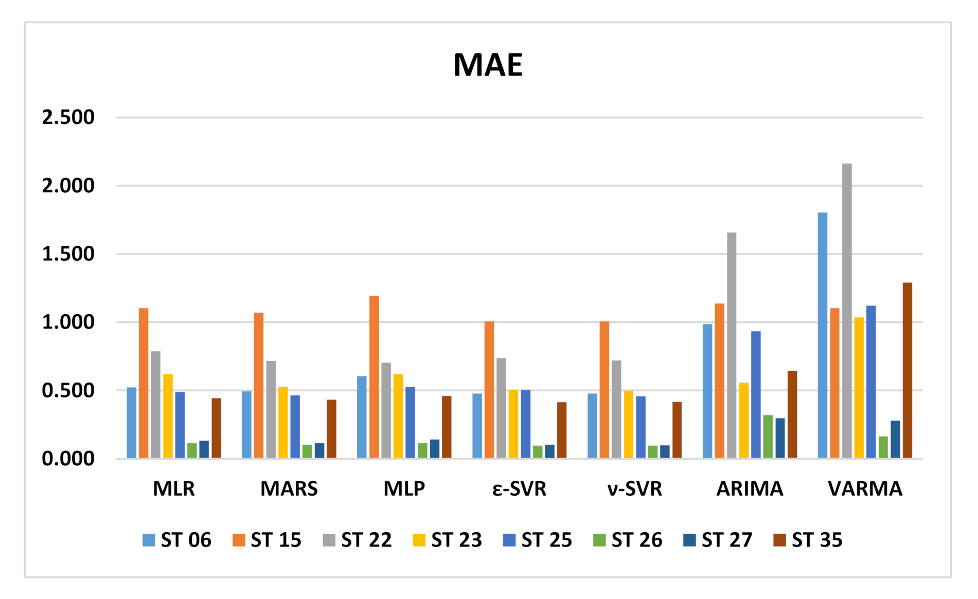
do the same for SVM, MLPNN with a single hidden layer with eight neurons, ARIMA and VARMA models, respectively. In the case of SVM, both ε-SVR and ν-SVR regressions were tested. Figure 2 shows a comparison of all RMSE values for all models and stations, the same is made for MAE in Figure 3 and BIAS in Figure 4.

For station 06, RMSE values are very similar and close to unity for the MLR, MARS and SVM models. The lowest value corresponds to MARS model with 0.936. RMSE value for MLP is slightly higher at 1.171. The highest values were reached with the time series models with 1.654 for ARIMA and 2.106 for VARMA. A similar behavior occurs with MAE, as the lowest value for the ε-SVR model is 0.478 and MLR, ν-SVR and MARS show values close to 0.5. MLP has a slightly higher value with 0.606 and the time series models reach the highest values, with 1.805 being the highest of the VARMA model. Regarding the bias error, all the models have negative values, so the prediction tends to be higher than the observed value. Again, the MLR, MARS and SVR models reached values close to zero and the time series models have a greater bias with values of 1.449 for VARMA.

RMSE values for station 15 are higher than those for station 06 overall. In this case, the lowest RMSE value was obtained for the ARIMA model, with 1.474. The SVR, MARS and MLR models have RMSE between 1.7 to 1.8 and the highest value was obtained for the MLP model, with 2.027. The MAE values are very close to each other, from 1.006 for ε-SVR to 1.195 for MLP, including time series models. However, the worst bias error values were obtained for the ARIMA model with −0.922 followed by VARMA with 0.6613. The rest of the models have a bias error close to zero, with positive values for MLR and MARS, together with VARMA.

Again, at station 22, the RMSE values are very similar for machine learning models, ranging from 1.220 for MLP to 1.304 for MLR. The time series models present much higher RMSE values, namely 3.008 for ARIMA and 2.642 for VARMA. The same occurs with the MAE values, which all remain at 0.7, varying from 0.704 for MLP to 0.788 for MLR. The MAE value for the time series models is 1.658 for ARIMA and the highest value is for VARMA, with 2.164. The bias error has values very close to zero for all machine learning models. MLR and ε-SVR have positive values, while the MARS, ν-SVR and MLP models have negative values of the bias error. Regarding the bias in time series models, it is 0.864 for VARMA and −1.6490 for ARIMA.

Station 23 does not have such a differentiated error pattern between machine learning models and early series models, and the error values are more clustered. The lowest value for RMSE was reached for both SVR models with 1.095 and the highest value for MLP, with 1.360. Something similar occurs with the MAE error. The lowest error was achieved for ν-SVR with 0.498 and the highest value for MLP, with 0.621. The lowest bias error was reached for MLR with ${10}^{-4}$ and the highest value for VARMA with 0.679, with positive values for MLR and MARS and negative for the rest of the models.

At station 25, the RMSE error ranges from 1.015 for the MARS model to 1.397 for the VARMA model. Time series models have slightly higher RMSE than machine learning models. Regarding MAE, the time series models have approximately twice the value of the other models, the lowest value being 0.458 for ν-SVR and the highest for VARMA, with 1.123. The same goes for the bias error. All bias errors in machine learning models are negative and close to zero with the lowest value for MLR. On the other hand, the time series models present positive values; that is, the observed value is greater than that predicted by these models, with the highest bias value for VARMA, with 0.579.

At station 26, the ARIMA model is the one that differs the most from the rest of the models, which show similar behavior for the three errors. The lowest value of RMSE was reached for the MARS and SVR models with 0.24, followed by MLP and MLR with 0.25 and 0.27 for VARMA. The ARIMA model has an RMSE of 0.36. The smallest MAE error was achieved in SVR, with 0.097. The rest of the models vary from 0.104 for MARS to 0.164 for VARMA, reaching 0.319 for the ARIMA model. The smallest bias error is for MLR, with a positive 5 × 10⁻⁶ value. In the rest of the models the values are negative, except ARIMA, which reached a value of 0.243.

All machine learning models show similar behavior at station 27, with the lowest RMSE value for the MARS model being 0.271. The time series models have a somewhat higher RMSE with a higher value for the ARIMA model, with 0.517. The lowest value of MAE is 0.100 and was achieved with the ν-SVR model. The behavior is similar to that of the RMSE error. The highest value was obtained for ARIMA, with 0.298. Regarding the bias error, the models that perform better are MLR and MARS, with positive values of 10 × 10⁻⁵. The rest of the models have a negative bias error and the highest value was obtained for the VARMA model, with −0.195.

The behavior of the RMSE error in station 35 was very similar for all models, acquiring the lowest value for ε-SVR with 0.880 and the highest value for ARIMA, with 1.088. Machine learning models have a similar MAE error, the smallest being 0.416 for ε-SVR. Time series models have a slightly larger MAE error of 0.643 for ARIMA. The bias error is negative for all models except for VARMA, being very close to zero and the lowest value on the order of −10 × 10⁻⁴ corresponds to MLR. The RVS models show a bias error of −0.02, while the bias error of the ARIMA model is −0.318.

At stations 15 and 23, the MLP model has a very high RMSE in relation to the machine learning models, compared to the homogeneity of the RMSE error performance in the rest of the stations. Station 35 has a very homogeneous RMSE error for all models. In stations 06 and 22, the machine learning models also have a homogeneous RMSE, but there is a clear difference with respect to the time series models, whose RMSE is higher. Station 15 has the highest RMSE and MAE in machine learning models, but this does not happen in time series models. Stations 26 and 27 have clearly lower RMSE and MAE values in all models, including time series models. The worst bias error for the ARIMA model is found at station 22. This model is the one that, together with VARMA, has the highest bias error for all stations, in general. The SVM models, both ε-SVR and ν-SVR, perform in a very similar way.

4. Conclusions

This paper studies the relationship between four predictors and benzene in order to establish predictions at eight stations in the community of Madrid, Spain, using seven mathematical models: MLR, MARS, ε-SVR, ν-SVR, MLP, ARIMA and VARMA.

Stations 06, 15, 22 and 35 are stations that are located in the city center and have observations with an average concentration of benzene higher than the rest of the stations located in the east, on the outskirts of the city or near the airport.

The models were evaluated using RMSE, MAE and bias. The validation of the machine learning models was carried out using k times the cross validation with k = 5 and with 20% of the observations for the time series models.

The results showed that, in general, machine learning models are more effective at predicting than time series models, but this does not happen at all stations, since at station 15 the lowest RMSE occurs in the VARMA model. The highest error values occur for the time series models, except at station 15, where they were obtained for the MLP model.

MLR, MARS, SVR and MLP follow similar behavior patterns for all stations and stations 26 and 27 show the lowest errors.

The time series models, ARIMA and VARMA, present greater variations in the values obtained for the stations, not following the same pattern as the machine learning models.