A Differential Game with Random Time Horizon and Discontinuous Distribution

Abstract

One class of differential games with random duration is considered. It is assumed that the duration of the game is a random variable with values from a given finite interval. The cumulative distribution function (CDF) of this random variable is assumed to be discontinuous with two jumps on the interval. It follows that the player’s payoff takes the form of the sum of integrals with different but adjoint time intervals. In addition, the first interval corresponds to the zero probability of the game to be finished, which results in terminal payoff on this interval. The method of construction optimal solution for the cooperative scenario of such games is proposed. The results are illustrated by the example of differential game of investment in the public stock of knowledge.

1. Introduction

Dynamic processes with many participants are well described by the differential game theory framework (e.g., for differential games see [1], also [2] in Russian, and their applications in economics in [3]). Meanwhile, a lot of natural processes (such as ecological dynamics) impose random components [4]. Thus, the assumption of the random nature of the processes’ time horizon allows constructing models even closer to reality [5]. Therefore, differential game models with random duration are of particular importance. This type of models was initially introduced in [6], where a differential game of pursuit with terminal payoff and stochastic terminal time was considered; the first problem formulation with integral payoff function and random time horizon with continuous distribution function was considered in [7] and later extended to the case of differential game with random time horizon and discounting in [8].

In this work, one class of differential games with a random time horizon is considered. It is assumed that the duration of the game is a random variable corresponding to the discontinuous cumulative distribution function (CDF). Particular classes of discontinuous models had been formulated in [9] for the case with only one jump and in [10] for the step form of the CDF. In this paper, the discontinuous structure of the CDF of the game implies that the game can not be interrupted until a certain point, then could stop either on the continuous interval or in the certain discrete-time moments. Moreover, the first interval corresponds to the zero probability of the game to be ended, which results in terminal payoff on this time interval. This game formulation leads to the fact that the player’s payoff takes the form of the sum of integrals with different, but adjoint time intervals and the problem can be considered in terms of hybrid differential games [11,12]. For more examples of games with regime switching see, e.g., [13,14,15].

The method of solution for such a wide class of problems by using dynamic programming methods [1], the maximum Pontryagin principle [16] and parametrization firstly was suggested in [17] for a class of differential games with random time horizon, with continuous but composite CDF, further generalized in [11]. Based on [11], a number of games with payoffs defined on adjoint time intervals were solved in [18,19].

In this paper, a method to construct optimal controls for the introduced class of games with discontiniuous CDF is proposed. This method refers to the idea of defining the connecting trajectory points at the edges of intervals as numeric parameters and usage of the maximum Pontryagin principle [16], after every interval. The numeric values for these points are obtained by maximization of total payoff under a dynamic programming approach on the interval. The method can also be used for a non-cooperative game scenario to find Nash equllibria and further exploit for a wide class of differential games with integral payoffs defined on different time intervals.

The results obtained in this work are illustrated by the game-theoretical model of investment to the public stock of knowledge [3] (also see [20]) modified accordingly to the described stochastic framework. The considered model refers to the unstable market conditions which bring a random nature to the process.

The paper is organized as follows. Section 2 is dedicated to the game formulation and main assumptions made to construct a feasible solution. The following Section 3 consists of the stock investment model specification. The optimization approach for the game formulation considered in the paper is proposed in Section 3 as well. In Section 4.1, the calculations for the adjoint time intervals are given. All the necessary details to reproduce this result of the work are written in Appendix A. Section 4.2 provides the dynamic programming approach to determine the numerical values of the state at the end points of the intervals. The limit case under the assumption of no jumps considered CDF is investigated in Section 5.1. Another limit case with assumption of step CDF is described in Section 5.2. The last Section presents a numeric example for the stock investment model.

2. Problem Formulation

Consider a differential game of n participants (players): ${\Gamma }^T(t_0,x_0)$. Let $N=\{1,\dots ,n\}$ be the set of players. Assume that the game starts at the initial moment $t_0$ and the initial state $x_0$; the duration of the game is a random variable such that it corresponds to the particular cumulative distribution function (CDF) described in the below notation. The following assumptions are made:

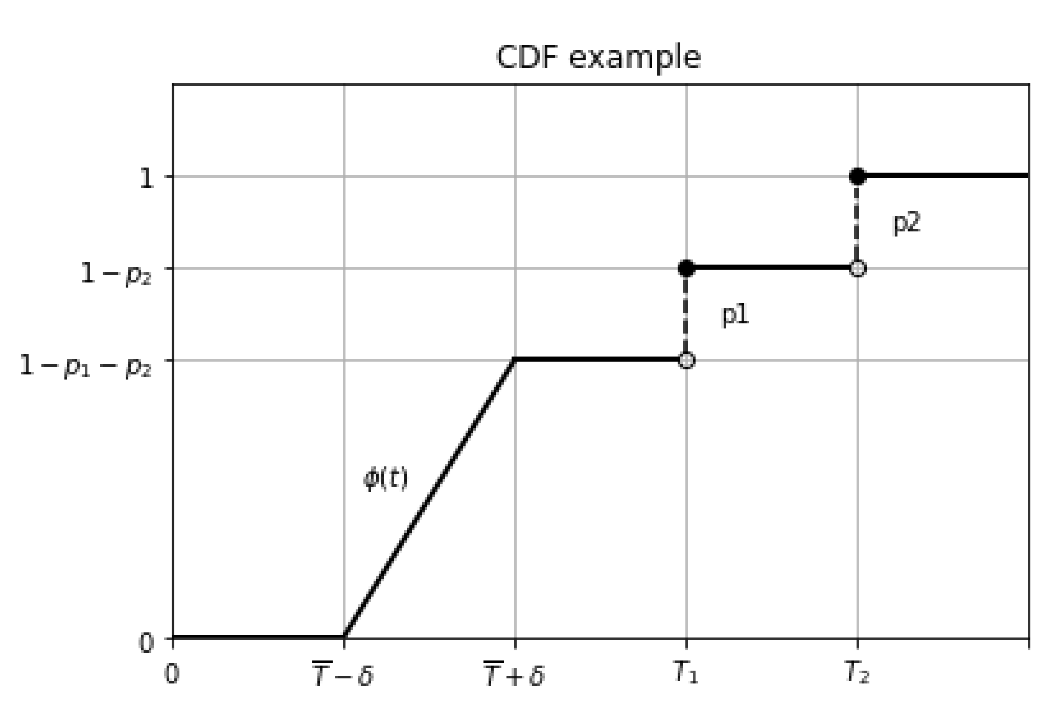
• the interval over which the game is played is $[t_0,T]\subset {\mathbb{R}}_{+}$, where $t_0\ge 0$ and T are random variables defined on the interval $[t_0,T_2]$, $T_2<\infty$. The random variable corresponds to the discontinuous CDF

  $$F\left(\tau \right)=\left\{\begin{array}{cc}0,\hfill & \mathrm{if}\tau <\overline{T}-\delta ,\hfill \\ \phi \left(\tau \right),\hfill & \mathrm{if}\overline{T}-\delta \le \tau <\overline{T}+\delta ,\hfill \\ 1-p_1-p_2,\hfill & \mathrm{if}\overline{T}+\delta \le \tau <T_1,\hfill \\ 1-p_2,\hfill & \mathrm{if}{T}_1\le \tau <T_2,\hfill \\ 1,\hfill & \mathrm{for}\tau \ge T_2,\hfill \end{array}\right.$$

  (1)

  where $\phi \left(\tau \right)$ is assumed to be an absolutely continuous non-decreasing function, $\phi (\overline{T}-\delta )=0,$ $\phi (\overline{T}+\delta )=1-p_1-p_2,$ $p_1>0$, $p_2>0$, $p_1+p_2\le 1$.
  The CDF of the random variable is assumed to be discontinuous with two jumps occurring on the bounded interval. The example of such CDF is given on Figure 1;
  

  Figure 1. The example of discrete distribution of random time horizon.
• the dynamic constraints of the game are given by

  $$\left\{\begin{array}{c}\dot{x}=g(x\left(t\right),u_1\left(t\right),\dots ,u_n\left(t\right)),\hfill \\ x\in R^h,x\left(t_0\right)=x_0.\hfill \end{array}\right.,$$

  (2)

  where the state Equation (2) are the ODEs whose solutions satisfy the standard existence and uniqueness requirements, which means that the function $g(x\left(t\right),u_1\left(t\right),\dots ,u_n\left(t\right))$ in (2) is a differentiable function on $[t_0;T_2]$;
• the controls $u_i\left(t\right)$ are open-loop strategies;
• the controls $u_i\left(t\right)$ belong to the sets of admissible controls ${\mathcal{U}}_i$, which consist of all measurable functions on the interval $[t_0,T_2]$, taking values in the set of admissible control values ${\mathbb{U}}_i$, which are in turn convex compact subsets of ${\mathbb{R}}^k$;
• the instantaneous payoff of the i-th player at the moment $\tau \in [t_0,T_2]$ is defined as $h_i(x\left(\tau \right),u_1\left(\tau \right),\dots ,u_n\left(\tau \right))$. To shorten the notation, we write

  $$h_i(x\left(\tau \right),u_1\left(\tau \right),\dots ,u_n\left(\tau \right))=h_i(x\left(\tau \right),u\left(\tau \right)),$$

  where $u\left(\tau \right)=\{u_1\left(\tau \right),\dots ,u_n\left(\tau \right)\}$;
• in the deterministic case the integral payoff is

  $$J_i(x_0,t_0,T_f,u)=\underset{t_0}{\overset{T_f}{\int }}{h}_i(x\left(t\right),u\left(t\right))dt,i=\overline{1,n},$$

  (3)

  where $T_f$ is a known moment of the end of the game, $T_f\in [t_0,T_2]$;
• in the case of random time horizon, the mathematical expectation of the integral payoff is considered. Thus, the i-th player’s integral functional is:

  $$K_i(x_0,t_0,T_2,u)=E\left(J_i\right)=\underset{t_0}{\overset{T_2}{\int }}\underset{t_0}{\overset{t}{\int }}{h}_i(x\left(\tau \right),u\left(\tau \right))d\tau dF\left(t\right),i=\overline{1,n}.$$

  (4)

It was obtained previously [10] that (4) can be written as follows

$$K_i(x_0,t_0,T_2,u)=\underset{t_0}{\overset{T_2}{\int }}{h}_i(x\left(t\right),u\left(t\right))(1-F\left(t\right))dt,i=\overline{1,n}.$$

(5)

Proposition 1.

For the considered game formulation, the payoff is a sum of functionals defined over four time intervals:

$$\begin{array}{cc}\hfill K_i(x_0,t_0,T_1,T_2,u)=\underset{t_0}{\overset{\overline{T}-\delta }{\int }}{h}_i(x\left(t\right),u\left(t\right))dt& +\underset{\overline{T}-\delta }{\overset{\overline{T}+\delta }{\int }}{h}_i(x\left(t\right),u\left(t\right))(1-\phi \left(t\right))dt\hfill \\ \hfill & +\underset{\overline{T}+\delta }{\overset{T_1}{\int }}{h}_i(x\left(t\right),u\left(t\right))(p_1+p_2)dt+\underset{T_1}{\overset{T_2}{\int }}{h}_i(x\left(t\right),u\left(t\right))p_{2}dt.\hfill \end{array}$$

(6)

Proof. 

The CDF of the random variable in the described game formulation is a piecewise function on the four time intervals. It is not hard to spot, that due to the zero probability of the game to be ended on the first interval $[t_0,\overline{T}-\delta ]$, the payoff of the player on this interval takes a deterministic form. The payoff on the other intervals is nothing but a mathematical expectation of the integration payoff corresponding to the particular form of the CDF on the interval. Thus, accordingly to (5) and proof in [10], the total payoff of the player could be written as the sum of four adjoint integrals (6). □

Obviously, the problem can be easily modified for the more general case with jumps at $T_1,T_2,\dots ,T_n$.

3. Model Example

Consider the model example in the frame of differential game formulation mentioned in the previous section. Namely, consider a so-called stock investment model described in [3] (also see [21]). There, n individuals invest in the stocks related to the particular industry. State variable $x\left(t\right)$ corresponds to the number of stocks held at the moment t, and $u_i\left(t\right)$ is the investment strategy of agent i at time t. The game dynamics take form of the accumulative process

$$\dot{x}\left(t\right)=\sum _{i=1}^N{u}_i\left(t\right),x\in R,u_i\in U\subseteq R,x\left(t_0\right)=x_0.$$

(7)

Assume that the instant payoff function is the linear-quadratic one, as each agent derives linear utility from the consumption of the stock

$$h_i(x\left(t\right),u\left(t\right))=q_{i}x\left(t\right)-r_i{u}_i^2\left(t\right),q_i>0,r_i>0.$$

(8)

Assume also that the CDF function of the game partly corresponds to a uniform distribution

$$F\left(\tau \right)=\left\{\begin{array}{cc}0,\hfill & \mathrm{if}\tau <\overline{T}-\delta ,\hfill \\ (1-p_1-p_2)\frac{t-\overline{T}+\delta }{2\delta },\hfill & \mathrm{for}\overline{T}-\delta \le \tau <\overline{T}+\delta ,\hfill \\ 1-p_1-p_2,\hfill & \mathrm{if}\overline{T}+\delta \le \tau <T_1,\hfill \\ 1-p_2,\hfill & \mathrm{if}{T}_1\le \tau <T_2,\hfill \\ 1,\hfill & \mathrm{if}\tau \ge T_2.\hfill \end{array}\right.$$

(9)

To further simplify the investigation, assume that the initial moment of the game is equal to zero: $t_0=0$.

Consider the cooperative form of the game. Assume that all participants decided to cooperate and, thus, unite their efforts to maximize the total payoff.

$$\sum _{i=1}^n{K}_i(x_0,t_0,T_1,T_2,u)\to \underset{u}{max}$$

The optimization problem can be solved using parametric method for four separate intervals. Over every interval, we use the Pontryagin maximum principle [16].

We start by introducing three yet undefined values of the state at the respective switching instants:

$$x_1,x_2,x_3\subseteq R.$$

Let $I_i$ denote the ith interval, $I_i\left(x_j\right)$ is the total payoff on interval i, which depends on the numeric parameter $x_j$. So, we obtain the following connected optimization problems:

$$\begin{array}{ccccc}\hfill & I_1:[0;\overline{T}-\delta ]\hfill & \hfill & \leftarrow \mathrm{both}\mathrm{sides}\mathrm{are}\mathrm{fixed}\hfill & \hfill \{x_0,x_1\}\\ \hfill & I_2:[\overline{T}-\delta ;\overline{T}+\delta ]\hfill & \hfill & \leftarrow \mathrm{both}\mathrm{sides}\mathrm{are}\mathrm{fixed}\hfill & \hfill \{x_1,x_2\}\\ \hfill & I_3:[\overline{T}+\delta ;T_1]\hfill & \hfill & \leftarrow \mathrm{both}\mathrm{sides}\mathrm{are}\mathrm{fixed}\hfill & \hfill \{x_2,x_3\}\\ \hfill & I_4:[T_1;T_2]\hfill & \hfill & \leftarrow \mathrm{only}\mathrm{one}\mathrm{side}\mathrm{is}\mathrm{fixed}\hfill & \hfill \left\{x_3\right\}\end{array}$$

To obtain the numeric value of every parameter $x_1,x_2,x_3$, the following algorithm based on dynamic programming principle can be used

$$I_1\left(x_1\right)+I_2(x_1,x_2)+I_3(x_2,x_3)+I_4\left(x_3\right)\to \underset{x_1,x_2,x_3}{max}$$

• $I_3(x_2,x_3)+I_4\left(x_3\right)\to {max}_{x_3}$ –compute $x_3$ parameterized by $x_2$;
• $I_2(x_1,x_2)+{max}_{x_3}\{I_3(x_2,x_3)+I_4\left(x_3\right)\}\to {max}_{x_2}$ –compute $x_2$ parameterized by $x_1$, while using the previously obtained expression for $x_3$ that depends on $x_2$;
• $I_1\left(x_1\right)+{max}_{x_2}\{I_2(x_1,x_2)+{max}_{x_3}\{I_3(x_2,x_3)+I_4\left(x_3\right)\}\}\to {max}_{x_1}$ –compute $x_1$.

Thus, all three numeric values for $x_1,x_2,x_3$ can be unambiguously obtained.

4. Computations

4.1. Intervals Calculations

In this section, the expressions for the optimal control and optimal trajectory are obtained under the assumption that three numeric parameters $x_1,x_2,x_3$ are given. The detailed calculations for all four intervals are presented in Appendix A. For every interval, the Pontryagin maximum principle (under the assumption of one side of interval fixed or both sides fixed) is used.

For the interval $I_1$, we obtain the following expressions for the optimal trajectory and controls:

$$\begin{array}{c}\hfill x^{*}{\left(t\right)}_{I_1}=\frac{(x_1-x_0)t}{(\overline{T}-\delta )}+\frac{1}{4}\widehat{q}t(\overline{T}-\delta -t)\sum _{i=1}^n\frac{1}{r_i}+x_0,\\ \hfill u_i^{*}{\left(t\right)}_{I_1}=\frac{x_1-x_0}{r_i{\sum }_{i=1}^n\frac{1}{r_i}(\overline{T}-\delta )}+\frac{\widehat{q}(\overline{T}-\delta )}{4r_i}-\frac{\widehat{q}t}{2r_i}.\end{array}$$

(10)

For the interval $I_2$, we have the following expressions for the optimal trajectory and controls:

$$\begin{array}{cc}\hfill x^{*}{\left(t\right)}_{I_2}& =\frac{\widehat{q}{\sum }_{i=1}^n\frac{1}{r_i}}{2{(1-p_1-p_2)}^2}\left({\delta }^2-\frac{\chi {\left(t\right)}^2}{4}\right)\hfill \\ \hfill +& \frac{2(x_2-x_1)(1-p_1-p_2)-\widehat{q}{\sum }_{i=1}^n\frac{1}{r_i}{\delta }^2(1+p_1+p_2)}{2ln(p_1+p_2)(1-p_1-p_2)}ln\frac{\chi \left(t\right)}{2\delta }+x_1,\hfill \\ \hfill u_i^{*}{\left(t\right)}_{I_2}& =\frac{\widehat{q}\chi \left(t\right)}{4r_i(1-p_1-p_2)}-\frac{2(x_2-x_1)(1-p_1-p_2)-\widehat{q}{\delta }^2{\sum }_{i=1}^n\frac{1}{r_i}(1+p_1+p_2)}{2r_i{\sum }_{i=1}^n\frac{1}{r_i}\chi \left(t\right)ln(p_1+p_2)},\hfill \end{array}$$

(11)

where $\chi \left(t\right)=2\delta -(1-p_1-p_2)(t-\overline{T}+\delta ).$

For the interval $I_3$, we obtain:

$$\begin{array}{cc}\hfill x^{*}{\left(t\right)}_{I_3}& =\sum _{i=1}^n\frac{1}{r_i}\left[\frac{(x_3-x_2)(t-\overline{T}-\delta )}{{\sum }_{i=1}^n\frac{1}{r_i}(T_1-\overline{T}-\delta )}+\frac{\widehat{q}(T_1-\overline{T}-\delta )(t-\overline{T}-\delta )}{4}-\frac{\widehat{q}{(t-\overline{T}-\delta )}^2}{4}\right]+x_2,\hfill \\ \hfill u_i^{*}{\left(t\right)}_{I_3}& =\frac{(x_3-x_2)}{r_i{\sum }_{i=1}^n\frac{1}{r_i}(T_1-\overline{T}-\delta )}+\frac{\widehat{q}(T_1+\overline{T}+\delta -2t)}{4r_i}.\hfill \end{array}$$

(12)

For the interval $I_4$, we obtain:

$$\begin{array}{cc}\hfill x^{*}{\left(t\right)}_{I_4}& =-\widehat{q}\sum _{i=1}^n\frac{1}{4r_i}\left[(t-T_1)(t+T_1-2T_2)\right]+x_3,\hfill \\ \hfill u_i^{*}{\left(t\right)}_{I_4}& =\frac{\widehat{q}(T_2-t)}{2r_i}.\hfill \end{array}$$

(13)

The expressions for optimal control on the intervals (10)–(13) are written under assumption of these controls belonging to the set of admissible controls ${\mathcal{U}}_i$. In other cases, the solution lies in the board of the compact set.

4.2. Computation of the Parameters $x_1,x_2,x_3$

As was written above, the connecting trajectory points at the boundary of intervals $x_1,x_2,x_3$ are obtained by the following algorithm.

$$I_1\left(x_1\right)+I_2(x_1,x_2)+I_3(x_2,x_3)+I_4\left(x_3\right)\to \underset{x_1,x_2,x_3}{max}$$

Using dynamic programming optimal principal

• $I_3(x_2,x_3)+I_4\left(x_3\right)\to {max}_{x_3}$ –compute $x_3$ parameterized by $x_2$;
• $I_2(x_1,x_2)+{max}_{x_3}\{I_3(x_2,x_3)+I_4\left(x_3\right)\}\to {max}_{x_2}$ –compute $x_2$ parameterized by $x_1$, while using the previously obtained expression for $x_3$ that depends on $x_2$;
• $I_1\left(x_1\right)+{max}_{x_2}\{I_2(x_1,x_2)+{max}_{x_3}\{I_3(x_2,x_3)+I_4\left(x_3\right)\}\}\to {max}_{x_1}$ –compute $x_1$.

Every expression is a linear-quadratic one in relation to $x_1,x_2\mathrm{or}{x}_3$ correspondingly. Thus, it is easy to obtain optimal values by using the first derivative of the expression. As a result, we obtain three linear equations, and after solving the system of these three equations, we obtain

$$\begin{array}{cc}\hfill x_1=& \frac{\widehat{q}(\overline{T}-\delta )(p_1(T_1-\overline{T})+p_2(T_2-\overline{T})+\frac{\overline{T}+\delta }{2}){\sum }_{i=1}^n\frac{1}{r_i}}{2}+x_0,\hfill \\ \hfill x_2=& \frac{\widehat{q}{\delta }^2{\sum }_{i=1}^n\frac{1}{r_i}}{2{(1-p_1-p_2)}^2}({(p_1+p_2)}^2(2ln(p_1+p_2)-1)+1)\hfill \\ & -\frac{\widehat{q}\delta {\sum }_{i=1}^n\frac{1}{r_i}ln(p_1+p_2)}{1-p_1-p_2}(p_1(T_1-\overline{T}-\delta )+p_2(T_2-\overline{T}-\delta ))+x_1,\hfill \\ \hfill x_3=& \frac{{\sum }_{i=1}^n\frac{1}{r_i}\widehat{q}(T_1-\overline{T}-\delta )}{2(p_1+p_2)}\left[\frac{(p_1+p_2)(T_1-\overline{T}-\delta )}{2}+p_2(T_2-T_1)\right]+x_2.\hfill \end{array}$$

(14)

5. Analysis of the Limiting Cases

5.1. Assumption of no Jumps in CDF

Consider the limit case of the game formulated in the paper. Namely, suppose that the probabilities $p_1,p_2$ which are responsible for the discontinuous structure of CDF function tend to zero

$$p_1\to 0,p_2\to 0.$$

This assumption leads to the situation when the CDF becomes a continuous function and the game cannot end after $\overline{T}+\delta$. Thus, we disregard the intervals $I_3,I_4$.

The dynamics and the instantaneous payoff function of the game remain the same

$$\begin{array}{c}\dot{x}\left(t\right)=\sum _{i=1}^N{u}_i\left(t\right),x\in R,u_i\in U\subseteq R,x\left(0\right)=x_0,h_i(x\left(t\right),u\left(t\right))=q_{i}x\left(t\right)-r_i{u}_i^2\left(t\right).\end{array}$$

The CDF function of the game takes form

$$F\left(\tau \right)=\left\{\begin{array}{cc}0,\hfill & \mathrm{for}\tau <\overline{T}-\delta \hfill \\ \frac{t-\overline{T}+\delta }{2\delta },\hfill & \mathrm{for}\overline{T}-\delta \le \tau <\overline{T}+\delta \hfill \\ 1,\hfill & \mathrm{for}\tau \ge \overline{T}+\delta .\hfill \end{array}\right.$$

This game formulation of stock investment game was investigated in [18]. Consider a cooperative form of the game:

$$\sum _{i=1}^n{K}_i(x_0,t_0,\overline{T}+\delta ,u)=\sum _{i=1}^n\underset{t_0}{\overset{\overline{T}-\delta }{\int }}{h}_i(x\left(t\right),u\left(t\right))dt+\sum _{i=1}^n\underset{\overline{T}-\delta }{\overset{\overline{T}+\delta }{\int }}{h}_i(x\left(t\right),u\left(t\right))(1-\frac{t-\overline{T}+\delta }{2\delta })dt\to max.$$

The optimization problem is solved using parametric method but with only one parameter $x_1\in R$.

$$\begin{array}{ccccc}\hfill & I_1:[0;\overline{T}-\delta ]\hfill & \hfill & \leftarrow \mathrm{both}\mathrm{sides}\mathrm{are}\mathrm{fixed}\hfill & \hfill \{x_0,x_1\}\\ \hfill & I_2:[\overline{T}-\delta ;\overline{T}+\delta ]\hfill & \hfill & \leftarrow \mathrm{only}\mathrm{one}\mathrm{side}\mathrm{is}\mathrm{fixed}\hfill & \hfill \left\{x_1\right\}\end{array}$$

To obtain the numeric value of parameter $x_1$, the following maximization problem must be solved

$$I_1\left(x_1\right)+I_2\left(x_1\right)\to \underset{x_1}{max}$$

The solution for this game is given in the form of optimal control, optimal trajectory and the numeric value of $x_1$. Using the Pontryagin maximum principle, it is not difficult to obtain the following expressions (denote them with superscript A)

$$\begin{array}{cc}\hfill x_1^A& =\frac{\widehat{q}({\overline{T}}^2-{\delta }^2){\sum }_{i=1}^n\frac{1}{r_i}}{4}+x_0,\hfill \\ \hfill u_i{\left(t\right)}_{I_1}^A& =\frac{\widehat{q}(\overline{T}-t)}{2r_i},u_i{\left(t\right)}_{I_2}^A=\frac{\widehat{q}(\overline{T}+\delta -t)}{4r_i}.\hfill \end{array}$$

(15)

$$\begin{array}{cc}\hfill x{\left(t\right)}_{I_1}^A& =\left(\frac{\left(x_1-x_0\right)t}{{\sum }_{i=1}^n\frac{1}{r_i}(\overline{T}-\delta )}+\frac{\widehat{q}(\overline{T}-\delta )}{4}t-\frac{\widehat{q}{t}^2}{4}\right)\sum _{i=1}^n\frac{1}{r_i}+x_0,\hfill \\ \hfill x{\left(t\right)}_{I_2}^A& =\frac{\widehat{q}{\sum }_{i=1}^n\frac{1}{r_i}}{4}\left((\overline{T}+\delta )t+\frac{{(\overline{T}-\delta )}^2-t^2}{2}\right)+x_0.\hfill \end{array}$$

(16)

From the other side, we can use the solution (10), (11) and (14) of the initial game described in Section 4 and set $p_1=0,p_2=0$.

The connection point $x_1$ (14) under assumption of $p_1$ and $p_2$ aiming to 0 coincides with the result obtained in (15):

$$\begin{array}{cc}\hfill x_1& =\frac{\widehat{q}(\overline{T}-\delta )(p_1(T_1-\overline{T})+p_2(T_2-\overline{T})+\frac{\overline{T}+\delta }{2}){\sum }_{i=1}^n\frac{1}{r_i}}{2}+x_0,\hfill \\ \hfill \underset{p_1\to 0,p_2\to 0}{lim}& \left(\frac{\widehat{q}(\overline{T}-\delta )(p_1(T_1-\overline{T})+p_2(T_2-\overline{T})+\frac{\overline{T}+\delta }{2}){\sum }_{i=1}^n\frac{1}{r_i}}{2}+x_0\right)=\frac{\widehat{q}({\overline{T}}^2-{\delta }^2){\sum }_{i=1}^n\frac{1}{r_i}}{4}+x_0=x_1^A.\hfill \end{array}$$

Similarly, the optimal control on the first interval (10) under the assumption of $p_1$ and $p_2$ tending to 0 also coincides with the control obtained for the reduced model (15):

$$\begin{array}{c}{u}_i^{*}{\left(t\right)}_{I_1}=\frac{x_1-x_0}{r_i{\sum }_{i=1}^n\frac{1}{r_i}(\overline{T}-\delta )}+\frac{\widehat{q}(\overline{T}-\delta )}{4r_i}-\frac{\widehat{q}t}{2r_i}=\frac{\frac{\widehat{q}({\overline{T}}^2-{\delta }^2){\sum }_{i=1}^n\frac{1}{r_i}}{4}}{r_i{\sum }_{i=1}^n\frac{1}{r_i}(\overline{T}-\delta )}+\frac{\widehat{q}(\overline{T}-\delta )}{4r_i}-\frac{\widehat{q}t}{2r_i}\hfill \\ \hfill =\frac{\widehat{q}(\overline{T}-t)}{2r_i}=u_i^{*}{\left(t\right)}_{I_1}^A.\end{array}$$

Optimal control on the second interval (11) under assumption of $p_1$ and $p_2$ aiming to 0 could be rewritten using the expression for $x_2$ obtained from (14):

$$\begin{array}{cc}\hfill x_2-x_1& =\frac{\widehat{q}{\delta }^2{\sum }_{i=1}^n\frac{1}{r_i}}{2{(1-p_1-p_2)}^2}({(p_1+p_2)}^2(2ln(p_1+p_2)-1)+1)\hfill \\ \hfill -& \frac{\widehat{q}\delta {\sum }_{i=1}^n\frac{1}{r_i}ln(p_1+p_2)}{1-p_1-p_2}(p_1(T_1-\overline{T}-\delta )+p_2(T_2-\overline{T}-\delta )).\hfill \\ \hfill \underset{p_1\to 0,p_2\to 0}{lim}(x_2-x_1)& =\frac{\widehat{q}{\delta }^2{\sum }_{i=1}^n\frac{1}{r_i}}{2}.\hfill \end{array}$$

Then we get the coincidence of optimal controls for the limiting case (16) and initial game (11):

$$\begin{array}{cc}\hfill u_i^{*}{\left(t\right)}_{I_2}& =\frac{\widehat{q}\chi \left(t\right)}{4r_i(1-p_1-p_2)}-\frac{2(x_2-x_1)(1-p_1-p_2)-\widehat{q}{\delta }^2{\sum }_{i=1}^n\frac{1}{r_i}(1+p_1+p_2)}{2r_i{\sum }_{i=1}^n\frac{1}{r_i}\chi \left(t\right)ln(p_1+p_2)},\hfill \\ \hfill \underset{p_1\to 0,p_2\to 0}{lim}& \left(\frac{\widehat{q}\chi \left(t\right)}{4r_i(1-p_1-p_2)}-\frac{2(x_2-x_1)(1-p_1-p_2)-\widehat{q}{\delta }^2{\sum }_{i=1}^n\frac{1}{r_i}(1+p_1+p_2)}{2r_i{\sum }_{i=1}^n\frac{1}{r_i}\chi \left(t\right)ln(p_1+p_2)}\right)\hfill \\ & =\frac{\widehat{q}(\overline{T}+\delta -t)}{4r_i}=u_i{\left(t\right)}_{I_2}^A.\hfill \end{array}$$

Optimal trajectory on the first interval (10) under assumption of $p_1$ and $p_2$ aiming to 0 also gives the results (16):

$$x^{*}{\left(t\right)}_{I_1}=\frac{(x_1-x_0)t}{(\overline{T}-\delta )}+\frac{1}{4}\widehat{q}t(\overline{T}-\delta -t)\sum _{i=1}^n\frac{1}{r_i}+x_0=x^{*}{\left(t\right)}_{I_1}^A.$$

Optimal trajectory function on the second interval under assumption of $p_1$ and $p_2$ aiming to 0 coincides with the corresponding result in (16):

$$\begin{array}{c}{x}^{*}{\left(t\right)}_{I_2}=\frac{\widehat{q}{\sum }_{i=1}^n\frac{1}{r_i}}{2{(1-p_1-p_2)}^2}\left({\delta }^2-\frac{\chi {\left(t\right)}^2}{4}\right)\hfill \\ \hfill +\frac{2(x_2-x_1)(1-p_1-p_2)-\widehat{q}{\sum }_{i=1}^n\frac{1}{r_i}{\delta }^2(1+p_1+p_2)}{2ln(p_1+p_2)(1-p_1-p_2)}ln(\frac{\chi \left(t\right)}{2\delta })+x_1,\end{array}$$

where $\chi \left(t\right)=2\delta -(1-p_1-p_2)(t-\overline{T}+\delta ).$ We have

$$\begin{array}{c}\underset{p_1\to 0,p_2\to 0}{lim}\left(\frac{\widehat{q}{\sum }_{i=1}^n\frac{1}{r_i}}{2{(1-p_1-p_2)}^2}\left({\delta }^2-\frac{\chi {\left(t\right)}^2}{4}\right)\right.\hfill \\ \hfill \left.+\frac{2(x_2-x_1)(1-p_1-p_2)-\widehat{q}{\sum }_{i=1}^n\frac{1}{r_i}{\delta }^2(1+p_1+p_2)}{2ln(p_1+p_2)(1-p_1-p_2)}ln(\frac{\chi \left(t\right)}{2\delta })+x_1\right)\hfill \\ \hfill =\frac{\widehat{q}{\sum }_{i=1}^n\frac{1}{r_i}}{4}\left((\overline{T}+\delta )t+\frac{{(\overline{T}-\delta )}^2-t^2}{2}\right)+x_0=x{\left(t\right)}_{I_2}^A.\end{array}$$

As we have shown, the solutions of the initial game and the reduced game coincide. Thus, the solution of the main game formulation described in Section 4 can be considered as the generalization of the game described in this Section.

5.2. Assumption of a Piece-Wise Constant CDF

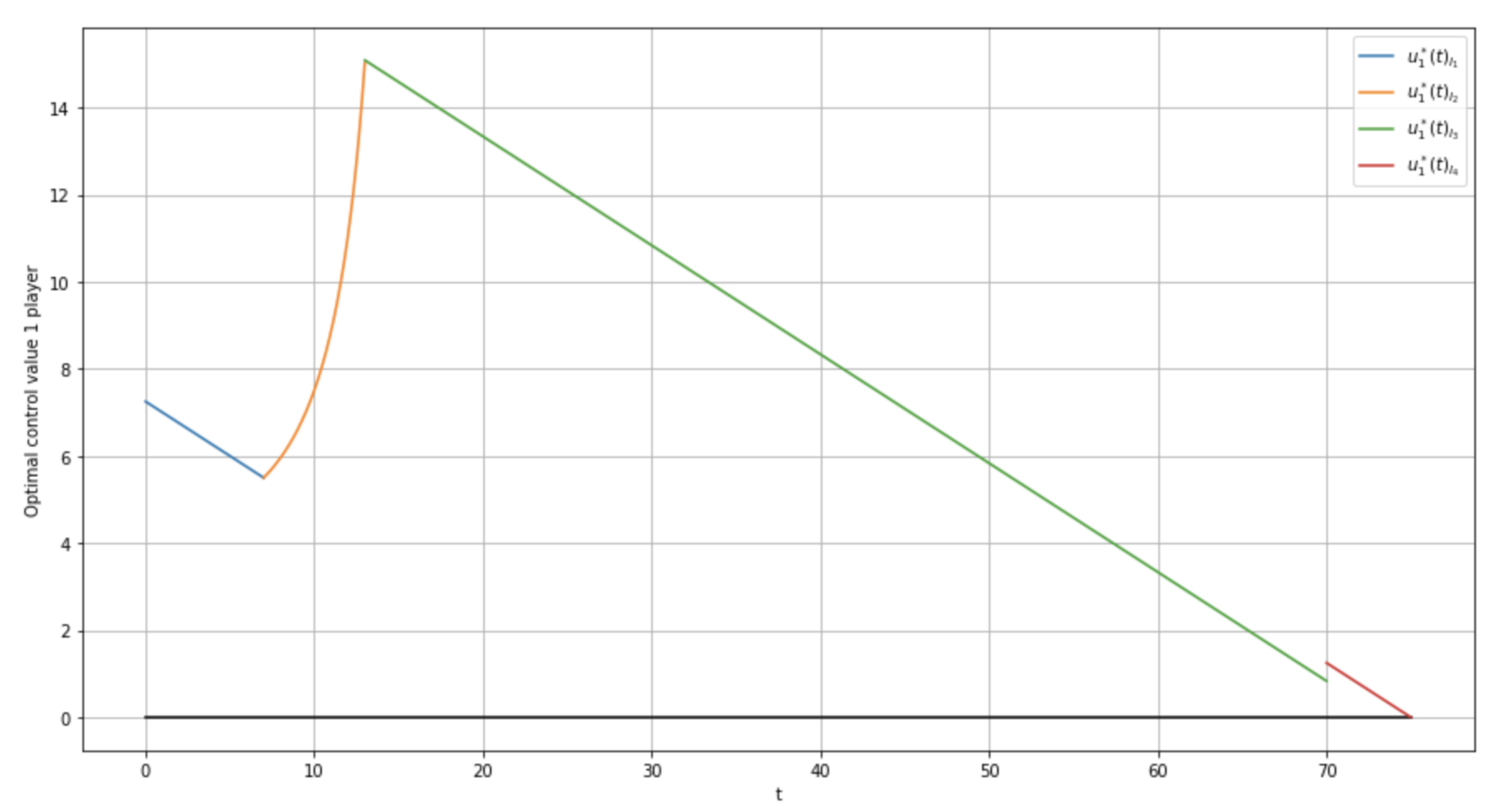
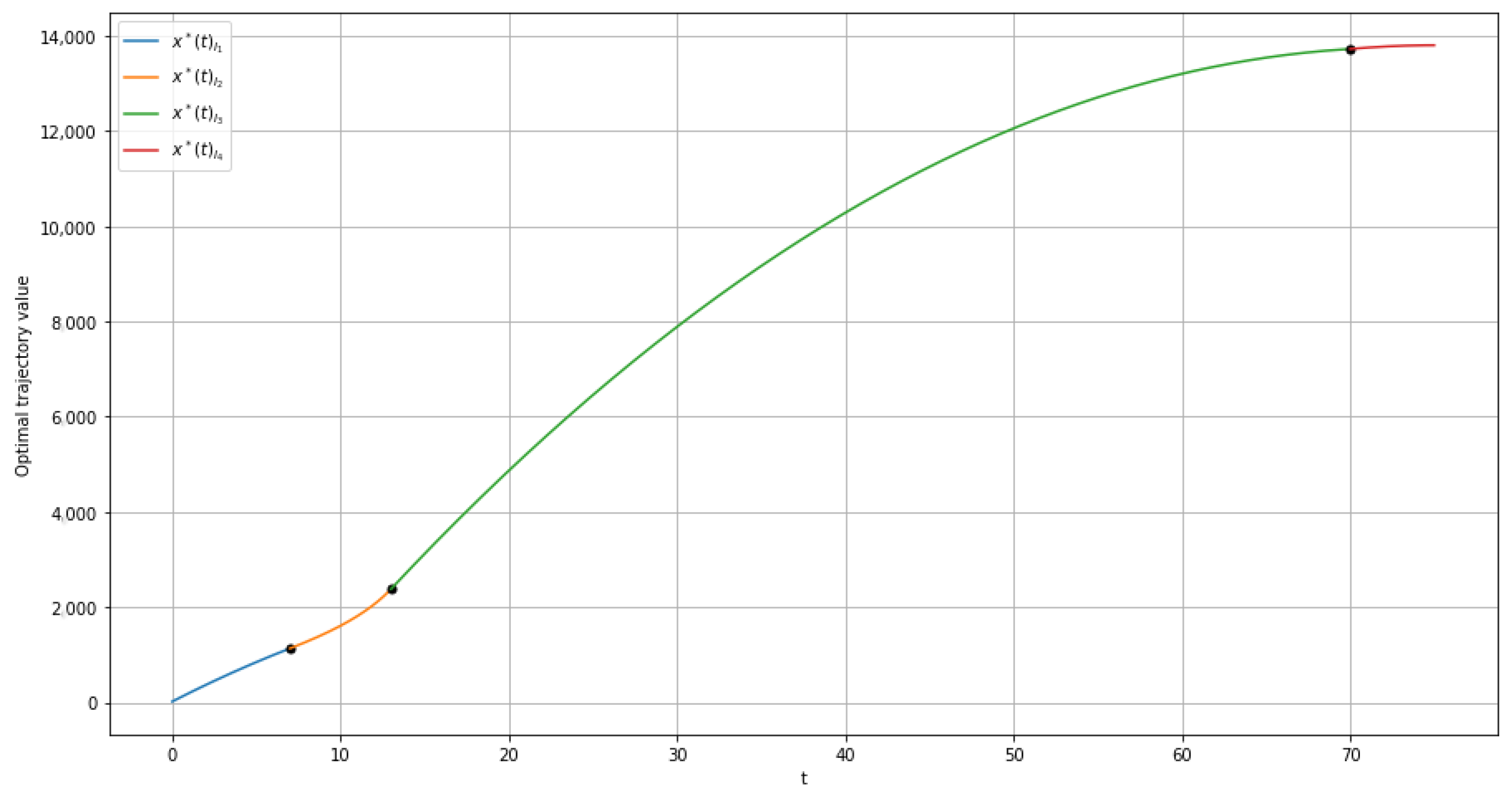
Consider another edge case of the game formulated in the paper. Now, suppose that the continuous part of (1) $\varphi \left(\tau \right)$ takes only zero values on all interval $[t_0,T_1]$. This assumption is equivalent to the following condition:

$$p_1+p_2=1.$$

In this case, CDF corresponds to discrete random variable T and becomes a step function with probabilities $p_1$ and $p_2$ of the game to be finished at time $T_1$ and $T_2$ correspondingly. Thus, there is a guaranteed terminal payoff on the interval $[t_0,T_1]$ and expected value for the interval $[T_1,T_2]$.

The dynamic and the instantaneous payoff function of the game remain, the same as

$$\begin{array}{c}\dot{x}\left(t\right)=\sum _{i=1}^N{u}_i\left(t\right),x\in R,u_i\in U\subseteq R,x\left(0\right)=x_0,\\ h_i(x\left(t\right),u\left(t\right))=q_{i}x\left(t\right)-r_i{u}_i^2\left(t\right).\end{array}$$

The CDF function of the game takes the step form:

$$F\left(\tau \right)=\left\{\begin{array}{cc}0,\hfill & \mathrm{if}\tau <T_1,\hfill \\ 1-p_2,\hfill & \mathrm{if}{T}_1\le \tau <T_2,\hfill \\ 1,\hfill & \mathrm{if}\tau \ge T_2.\hfill \end{array}\right.$$

This game formulation of differential game with discrete random time horizon was investigated in [22]. Consider cooperative form of the game:

$$\sum _{i=1}^n{K}_i(x_0,t_0,T_1,T_2,u)=\sum _{i=1}^n\underset{t_0}{\overset{T_1}{\int }}{h}_i(x\left(t\right),u\left(t\right))dt+p_2\sum _{i=1}^n\underset{T_1}{\overset{T_2}{\int }}{h}_i(x\left(t\right),u\left(t\right))dt\to max.$$

The optimization problem is solved using the parametric method, but only with one parameter $x_3\in R$:

$$\begin{array}{ccccc}\hfill & I_{1,2,3}:[0;T_1]\hfill & \hfill & \leftarrow \mathrm{both}\mathrm{sides}\mathrm{are}\mathrm{fixed}\hfill & \hfill \{x_0,x_3\}\\ \hfill & I_4:[T_1;T_2]\hfill & \hfill & \leftarrow \mathrm{only}\mathrm{one}\mathrm{side}\mathrm{is}\mathrm{fixed}\hfill & \hfill \left\{x_3\right\}\end{array}$$

To obtain the numeric value of parameter $x_3$, the following maximization problem must be solved

$$I_{1,2,3}\left(x_3\right)+I_4\left(x_3\right)\to \underset{x_3}{max}$$

The solution for this game is given in the form of optimal control, optimal trajectory and the numeric value of $x_3$. Using the Pontryagin maximum principle, we obtain the following expressions (denote them with superscript B):

$$x_3^B=\frac{\widehat{q}{\sum }_{i=1}^n\frac{1}{r_i}{T}_1}{2}\left[(T_2-T_1)p_2+\frac{T_1}{2}\right]+x_0.$$

Note that optimal control and optimal trajectory are the same over all three intervals $I_1,I_2,I_3$:

$$u_i{\left(t\right)}_{I_1,I_2,I_3}^B=\frac{\widehat{q}}{2r_i}\left[T_1{p}_1+T_2{p}_2-t\right].$$

$$x{\left(t\right)}_{I_1,I_2,I_3}^B=\frac{\widehat{q}{\sum }_{i=1}^n\frac{1}{r_i}}{2}\left[T_1{p}_{1}t+T_2{p}_{2}t-\frac{t^2}{2}\right]+x_0.$$

(17)

For the interval $I_4$, we obtain:

$$\begin{array}{cc}\hfill u_i{\left(t\right)}_{I_4}^B& =\frac{\widehat{q}(T_2-t)}{2r_i},\hfill \\ \hfill x{\left(t\right)}_{I_4}^B& =-\widehat{q}\sum _{i=1}^n\frac{1}{4r_i}(t-T_1)(t+T_1-2T_2)+x_3.\hfill \end{array}$$

From the expression for optimal trajectory (17), we can obtain the following points:

$$\begin{array}{c}\hfill x_1^B=x{(\overline{T}-\delta )}_{I_1,I_2,I_3}^B=\frac{\widehat{q}{\sum }_{i=1}^n\frac{1}{r_i}(\overline{T}-\delta )}{2}\left[p_1{T}_1+p_2{T}_2-\frac{\overline{T}-\delta }{2}\right]+x_0,\\ \hfill x_2^B=x{(\overline{T}+\delta )}_{I_1,I_2,I_3}^B=\frac{\widehat{q}{\sum }_{i=1}^n\frac{1}{r_i}(\overline{T}+\delta )}{2}\left[p_1{T}_1+p_2{T}_2-\frac{\overline{T}+\delta }{2}\right]+x_0.\end{array}$$

From the other side, we can use the solution (10)–(14) of the initial game described in Section 4 and calculate the limit under condition of $(p_1+p_2)\to 1$. Below, we use L’Hopital’s rule to compute the limits.

For the connectivity point $x_1$ under assumption of $p_1+p_2\to 1$, we obtain the results:

$$\begin{array}{cc}\hfill x_1& =\frac{\widehat{q}(\overline{T}-\delta )(p_1(T_1-\overline{T})+p_2(T_2-\overline{T})+\frac{\overline{T}+\delta }{2}){\sum }_{i=1}^n\frac{1}{r_i}}{2}+x_0,\hfill \\ \hfill & \underset{(p_1+p_2)\to 1}{lim}\left(\frac{\widehat{q}(\overline{T}-\delta )(p_1(T_1-\overline{T})+p_2(T_2-\overline{T})+\frac{\overline{T}+\delta }{2}){\sum }_{i=1}^n\frac{1}{r_i}}{2}+x_0\right)\hfill \\ \hfill & =\frac{\widehat{q}{\sum }_{i=1}^n\frac{1}{r_i}(\overline{T}-\delta )}{2}\left[p_1{T}_1+p_2{T}_2-\frac{\overline{T}-\delta }{2}\right]+x_0=x_1^B.\hfill \end{array}$$

Similarly, for $x_2$ and $x_3$, we have:

$$\begin{array}{cc}\hfill x_2& =\frac{\widehat{q}{\delta }^2{\sum }_{i=1}^n\frac{1}{r_i}}{2{(1-p_1-p_2)}^2}({(p_1+p_2)}^2(2ln(p_1+p_2)-1)+1)\hfill \\ \hfill -& \frac{\widehat{q}\delta {\sum }_{i=1}^n\frac{1}{r_i}ln(p_1+p_2)}{1-p_1-p_2}(p_1(T_1-\overline{T}-\delta )+p_2(T_2-\overline{T}-\delta ))+x_1.\hfill \\ \hfill \underset{(p_1+p_2)\to 1}{lim}& \left(\frac{\widehat{q}{\delta }^2{\sum }_{i=1}^n\frac{1}{r_i}}{2{(1-p_1-p_2)}^2}({(p_1+p_2)}^2(2ln(p_1+p_2)-1)+1)\right.\hfill \\ \hfill & \left.-\frac{\widehat{q}\delta {\sum }_{i=1}^n\frac{1}{r_i}ln(p_1+p_2)}{1-p_1-p_2}(p_1(T_1-\overline{T}-\delta )+p_2(T_2-\overline{T}-\delta ))+x_1\right)\hfill \\ \hfill & =\frac{\widehat{q}{\sum }_{i=1}^n\frac{1}{r_i}(\overline{T}+\delta )}{2}\left[p_1{T}_1+p_2{T}_2-\frac{\overline{T}+\delta }{2}\right]+x_0=x_2^B,\hfill \\ \hfill x_3& =\frac{{\sum }_{i=1}^n\frac{1}{r_i}\widehat{q}(T_1-\overline{T}-\delta )}{2(p_1+p_2)}\left[\frac{(p_1+p_2)(T_1-\overline{T}-\delta )}{2}+p_2(T_2-T_1)\right]+x_2.\hfill \end{array}$$

So, we obtain:

$$\begin{array}{c}\underset{(p_1+p_2)\to 1}{lim}\left(\frac{{\sum }_{i=1}^n\frac{1}{r_i}\widehat{q}(T_1-\overline{T}-\delta )}{2(p_1+p_2)}\left[\frac{(p_1+p_2)(T_1-\overline{T}-\delta )}{2}+p_2(T_2-T_1)\right]+x_2\right)\hfill \\ \hfill =\frac{\widehat{q}{\sum }_{i=1}^n\frac{1}{r_i}{T}_1}{2}\left[(T_2-T_1)p_2+\frac{T_1}{2}\right]+x_0=x_3^B.\end{array}$$

Optimal controls on the first interval under assumption of $(p_1+p_2)\to 1$ and the condition $x_1=x_1^B$ coincide both for the limiting and the initial cases:

$$\begin{array}{c}{u}_i^{*}{\left(t\right)}_{I_1}=\frac{x_1-x_0}{r_i{\sum }_{i=1}^n\frac{1}{r_i}(\overline{T}-\delta )}+\frac{\widehat{q}(\overline{T}-\delta )}{4r_i}-\frac{\widehat{q}t}{2r_i}=\frac{\frac{\widehat{q}{\sum }_{i=1}^n\frac{1}{r_i}(\overline{T}-\delta )}{2}\left[p_1{T}_1+p_2{T}_2-\frac{\overline{T}-\delta }{2}\right]}{r_i{\sum }_{i=1}^n\frac{1}{r_i}(\overline{T}-\delta )}+\frac{\widehat{q}(\overline{T}-\delta )}{4r_i}\hfill \\ \hfill -\frac{\widehat{q}t}{2r_i}=\frac{\widehat{q}}{2r_i}\left[T_1{p}_1+T_2{p}_2-t\right]=u_i{\left(t\right)}_{I_1,I_2,I_3}^B.\end{array}$$

Optimal control on the second interval under assumption of $(p_1+p_2)\to 1$ is rewritten using the expression for $x_2=x_2^B$:

$$u_i^{*}{\left(t\right)}_{I_2}=\frac{\widehat{q}\chi \left(t\right)}{4r_i(1-p_1-p_2)}-\frac{2(x_2-x_1)(1-p_1-p_2)-\widehat{q}{\delta }^2{\sum }_{i=1}^n\frac{1}{r_i}(1+p_1+p_2)}{2r_i{\sum }_{i=1}^n\frac{1}{r_i}\chi \left(t\right)ln(p_1+p_2)},$$

So again we have:

$$\begin{array}{cc}\hfill \underset{(p_1+p_2)\to 1}{lim}& \left(\frac{\widehat{q}\chi \left(t\right)}{4r_i(1-p_1-p_2)}-\frac{2(x_2-x_1)(1-p_1-p_2)-\widehat{q}{\delta }^2{\sum }_{i=1}^n\frac{1}{r_i}(1+p_1+p_2)}{2r_i{\sum }_{i=1}^n\frac{1}{r_i}\chi \left(t\right)ln(p_1+p_2)}\right)\hfill \\ & =\frac{\widehat{q}}{2r_i}\left[T_1{p}_1+T_2{p}_2-t\right]=u_i{\left(t\right)}_{I_1,I_2,I_3}^B.\hfill \end{array}$$

For the third interval, and taking in mind that $x_3$ depends on $p_1$ and $p_2$, we obtain:

$$\begin{array}{cc}\hfill u_i^{*}{\left(t\right)}_{I_3}& =\frac{(x_3-x_2)}{r_i{\sum }_{i=1}^n\frac{1}{r_i}(T_1-\overline{T}-\delta )}+\frac{\widehat{q}(T_1+\overline{T}+\delta -2t)}{4r_i},\hfill \\ \hfill \underset{(p_1+p_2)\to 1}{lim}& \left(\frac{(x_3-x_2)}{r_i{\sum }_{i=1}^n\frac{1}{r_i}(T_1-\overline{T}-\delta )}+\frac{\widehat{q}(T_1+\overline{T}+\delta -2t)}{4r_i}\right)\hfill \\ & =\frac{\widehat{q}}{2r_i}\left[T_1{p}_1+T_2{p}_2-t\right]=u_i{\left(t\right)}_{I_1,I_2,I_3}^B.\hfill \end{array}$$

For the last interval, the expression is the same:

$$u_i^{*}{\left(t\right)}_{I_4}=\frac{\widehat{q}(T_2-t)}{2r_i}=u_i{\left(t\right)}_{I_4}^B.$$

Optimal trajectory on the first interval under assumption of $(p_1+p_2)\to 1$ and the condition $x_1=x_1^B$ has the form:

$$\begin{array}{c}{x}^{*}{\left(t\right)}_{I_1}=\frac{(x_1-x_0)t}{(\overline{T}-\delta )}+\frac{1}{4}\widehat{q}t(\overline{T}-\delta -t)\sum _{i=1}^n\frac{1}{r_i}+x_0\hfill \\ \hfill =\frac{\widehat{q}{\sum }_{i=1}^n\frac{1}{r_i}}{2}\left[T_1{p}_{1}t+T_2{p}_{2}t-\frac{t^2}{2}\right]+x_0=x{\left(t\right)}_{I_1,I_2,I_3}^B.\end{array}$$

Optimal trajectory on the second interval under assumption of $(p_1+p_2)\to 1$ and $x_2=x_2^B$ is as follows:

$$\begin{array}{c}{x}^{*}{\left(t\right)}_{I_2}=\frac{\widehat{q}{\sum }_{i=1}^n\frac{1}{r_i}}{2{(1-p_1-p_2)}^2}\left({\delta }^2-\frac{\chi {\left(t\right)}^2}{4}\right)\hfill \\ \hfill +\frac{2(x_2-x_1)(1-p_1-p_2)-\widehat{q}{\sum }_{i=1}^n\frac{1}{r_i}{\delta }^2(1+p_1+p_2)}{2ln(p_1+p_2)(1-p_1-p_2)}ln(\frac{\chi \left(t\right)}{2\delta })+x_1,\end{array}$$

where $\chi \left(t\right)=2\delta -(1-p_1-p_2)(t-\overline{T}+\delta ).$ Then, we obtain:

$$\begin{array}{c}\underset{(p_1+p_2)\to 1}{lim}\left(\frac{\widehat{q}{\sum }_{i=1}^n\frac{1}{r_i}}{2{(1-p_1-p_2)}^2}\left({\delta }^2-\frac{\chi {\left(t\right)}^2}{4}\right)\right.\hfill \\ \left.+\frac{2(x_2-x_1)(1-p_1-p_2)-\widehat{q}{\sum }_{i=1}^n\frac{1}{r_i}{\delta }^2(1+p_1+p_2)}{2ln(p_1+p_2)(1-p_1-p_2)}ln(\frac{\chi \left(t\right)}{2\delta })+x_1\right)\\ \hfill =\frac{\widehat{q}{\sum }_{i=1}^n\frac{1}{r_i}}{2}\left[T_1{p}_{1}t+T_2{p}_{2}t-\frac{t^2}{2}\right]+x_0=x{\left(t\right)}_{I_1,I_2,I_3}^B.\end{array}$$

We also obtain the optimal trajectory on the third interval under assumption of $(p_1+p_2)\to 1$ and $x_3=x_3^B$:

$$\begin{array}{c}\hfill x^{*}{\left(t\right)}_{I_3}=\sum _{i=1}^n\frac{1}{r_i}\left[\frac{(x_3-x_2)(t-\overline{T}-\delta )}{{\sum }_{i=1}^n\frac{1}{r_i}(T_1-\overline{T}-\delta )}+\frac{\widehat{q}(T_1-\overline{T}-\delta )(t-\overline{T}-\delta )}{4}-\frac{\widehat{q}{(t-\overline{T}-\delta )}^2}{4}\right]+x_2.\end{array}$$

Then

$$\begin{array}{c}\underset{(p_1+p_2)\to 1}{lim}\left(\sum _{i=1}^n\frac{1}{r_i}\left[\frac{(x_3-x_2)(t-\overline{T}-\delta )}{{\sum }_{i=1}^n\frac{1}{r_i}(T_1-\overline{T}-\delta )}+\frac{\widehat{q}(T_1-\overline{T}-\delta )(t-\overline{T}-\delta )}{4}-\frac{\widehat{q}{(t-\overline{T}-\delta )}^2}{4}\right]+x_2\right)\hfill \\ \hfill =\frac{\widehat{q}{\sum }_{i=1}^n\frac{1}{r_i}}{2}\left[T_1{p}_{1}t+T_2{p}_{2}t-\frac{t^2}{2}\right]+x_0=x{\left(t\right)}_{I_1,I_2,I_3}^B.\end{array}$$

On the last interval, we have

$$x^{*}{\left(t\right)}_{I_4}=-\widehat{q}\sum _{i=1}^n\frac{1}{4r_i}\left[(t-T_1)(t+T_1-2T_2)\right]+x_3=x{\left(t\right)}_{I_4}^B.$$

As can be seen, the results coincide as well as in the edge case under assumption of no jumps. Thus, the solution of the main game formulation described in Section 4 could be considered as the generalization of the game described in this Section as well.

6. Numeric Example

This section is devoted to the particular numeric example of the stock investment game considered in the paper. Assume the following values of parameters

$$\begin{array}{cccc}\hfill & N=3\hfill & \hfill -& \mathrm{number}\mathrm{of}\mathrm{players}\hfill \\ \hfill & x_0=20\hfill & \hfill -& \mathrm{initial}\mathrm{number}\mathrm{of}\mathrm{stocks}\hfill \\ \hfill & t_0=0\hfill & \hfill -& \mathrm{initial}\mathrm{time}\hfill \\ \hfill & T=10,d=3,T_1=70,T_2=75\hfill & \hfill -& \mathrm{time}\mathrm{structure}\mathrm{parameters}\hfill \\ \hfill & q_1=1,q_2=3,q_3=6,\hfill & \hfill -& \mathrm{values}\mathrm{of}\mathrm{coefficients}\mathrm{from}\mathrm{payoff}\hfill \\ \hfill & r_1=20,r_2=1,r_3=4\hfill & \\ \hfill & p_1=0.1,p_2=0.2\hfill & \hfill -& \mathrm{probabilities}\mathrm{to}\mathrm{stop}\mathrm{the}\mathrm{game}\mathrm{at}{T}_1,T_2\hfill \end{array}$$

The cumulative distribution function (CDF) is defined according to (9).

Assume also that the set of admissible controls corresponds to the interval

$${\mathbb{U}}_i=[0;U],U<\infty .$$

The optimal control of the first player is presented in Figure 2. This function is a piecewise function defined on four separate intervals. The optimal control’s values belong to the predefined set of admissible control values.

Figure 2. The optimal control of the first player on four time subintervals.

The graphs for the other two players differ in minor details and show a similar picture with the controls belonging to the admissible set.

The optimal trajectory is presented in Figure 3. The trajectory is a continuous function defined on all four time subintervals. The bold black dots represent the connectivity points $x_1,x_2,x_3$ calculated in the previous section.

Figure 3. The optimal trajectory on four time subintervals connected by connectivity points—bold black dots $x_1,x_2,x_3$ correspondingly.

The evolution of the trajectory in Figure 3 is consistent with the intuitive understanding that it should be a non-decreasing continuous function. In contrast, Figure 2 shows the function for optimal investments, which should not satisfy the property of monotonicity and continuity, but should belong to a compact set, as shown in Figure 2.

7. Conclusions

In this work, a special class of differential games with random duration and discontinuous CDF was studied. The method to construct an optimal solution based on the consideration of separate adjoint time intervals is proposed. The analytical formulas of optimal control for every player and the optimal trajectory of the game are obtained. The numeric example is given and illustrated in the form of graphs.

In addition to the general formulation for the optimal solution we considered a number of special cases and shown that all considered cases agree well with the general formulation and can be derived from it. This proves the validity of our findings and extends the class of possible problems to be addressed within this framework.

The future research will consist, in particular, in studying the non-cooperative form of the game and time-consistency problem for the cooperative form of the game. In addition, we are going to investigate the Stackelberg equilibrium [23] for the considered game formulation.

References

1. Basar, T.; Olsder, G. Dynamic Noncooperative Game Theory; SIAM: New York, NY, USA, 1999. [Google Scholar]
2. Petrosyan, L.; Danilov, N. Cooperative Differential Games and THEIR Applications; Izd. Tomskogo University: Tomsk, Russia, 1982. [Google Scholar]
3. Dockner, E.J.; Jørgensen, S.; Long, N.V.; Sorger, G. Differential Games in Economics and Management Science. In Cambridge Books; Cambridge University Press: Cambridge, UK, 2000. [Google Scholar]
4. Yeung, D.; Petrosyan, L. Cooperative Stochastic Differential Games; Springer Science, Business Media: Berlin/Heidelberg, Germany, 2006. [Google Scholar]
5. Yaari, M. Uncertain lifetime, life insurance, and the theory of the consumer. Rev. Econ. Stud. 1965, 32, 137–150. [Google Scholar] [CrossRef]
6. Petrosyan, L.; Murzov, N. Game-theoretic problems of mechanics. Litovsk. Math. Sb. 1966, 7, 423–433. [Google Scholar]
7. Petrosyan, L.; Shevkoplyas, E. Cooperative differential games with stochastic time. Vestn. Petersburg Univ. Math. 2000, 33, 18–23. [Google Scholar]
8. Marin-Solano, J.; Shevkoplyas, E. Non-constant discounting and differential games with random time horizon. Automatica 2011, 47, 2626–2638. [Google Scholar] [CrossRef]
9. Gromova, E.; Malakhova, A.; Palestini, A. Payoff Distribution in a Multi-Company Extraction Game with Uncertain Duration. Mathematics 2018, 6, 165. [Google Scholar] [CrossRef] [Green Version]
10. Gromova, E.; Tur, A. On the form of integral payoff in differential games with random duration. In Proceedings of the 2017 XXVI International Conference on Information, Communication and Automation Technologies (ICAT), Sarajevo, Bosnia-Herzegovina, 26–28 October 2017; pp. 1–6. [Google Scholar]
11. Gromov, D.; Gromova, E. On a Class of Hybrid Differential Games. Dyn. Games Appl. 2017, 7, 266–288. [Google Scholar] [CrossRef]
12. Reddy, P.V.; Schumacher, J.M.; Engwerda, J.C. Analysis of optimal control problems for hybrid systems with one state variable. SIAM J. Control. Optim. 2020, 58, 3262–3292. [Google Scholar] [CrossRef]
13. Bonneuil, N.; Boucekkine, R. Optimal transition to renewable energy with threshold of irreversible pollution. Eur. J. Oper. Res. 2016, 248, 257–262. [Google Scholar] [CrossRef] [Green Version]
14. Elliott, R.J.; Siu, T.K. A stochastic differential game for optimal investment of an insurer with regime switching. Quant. Financ. 2011, 11, 365–380. [Google Scholar] [CrossRef]
15. Reddy, P.; Schumacher, J.; Engwerda, J. Optimal management with hybrid dynamics—The shallow lake problem. In Mathematical Control Theory I; Springer: Berlin/Heidelberg, Germany, 2015; pp. 111–136. [Google Scholar]
16. Pontryagin, L.; Boltyanskii, V.; Gamkrelidze, R.; Mishchenko, E. The Mathematical Theory of Optimal Processes; Interscience: New York, NY, USA, 1962. [Google Scholar]
17. Gromov, D.; Gromova, E. Differential games with random duration: A hybrid systems formulation. Contrib. Game Theory Manag. 2014, 7, 104–119. [Google Scholar]
18. Tur, A.V.; Magnitskaya, N.G. Feedback and Open-Loop Nash Equilibria in a Class of Diferential Games with Random Duration. Contrib. Game Theory Manag. 2020, 13, 415–426. [Google Scholar] [CrossRef]
19. Gromova, E.; Magnitskaya, N. Solution of the differential game with hybrid structure. Contrib. Game Theory Manag. 2019, 12, 159–176. [Google Scholar]
20. Feichtinger, G.; Jørgensen, S. Differential game models in management science. Eur. J. Oper. Res. 1983, 14, 137–155. [Google Scholar] [CrossRef]
21. Jørgensen, S.; Zaccour, G. Developments in differential game theory and numerical methods: Economic and management applications. Comput. Manag. Sci. 2007, 4, 159–181. [Google Scholar] [CrossRef]
22. Malakhova, A.P.; Gromova, E.V. Strongly Time-Consistent Core in Differential Games with Discrete Distribution of Random Time Horizon. Math. Appl. 2018, 46, 197–209. [Google Scholar] [CrossRef]
23. Abdel-Wahab, O.; Bentahar, J.; Otrok, H.; Mourad, A. Resource-Aware Detection and Defense System Against Multi-Type Attacks in the Cloud: Repeated Bayesian Stackelberg Game. IEEE Trans. Dependable Secur. Comput. 2019. [Google Scholar] [CrossRef]