New Computational Geometry Methods Applied to Solve Complex Problems of Radiative Transfer


Abstract
1. Introduction
1.1. Form Factors
1.2. Configuration Factors
2. Symbolic Calculus of Basic Elements
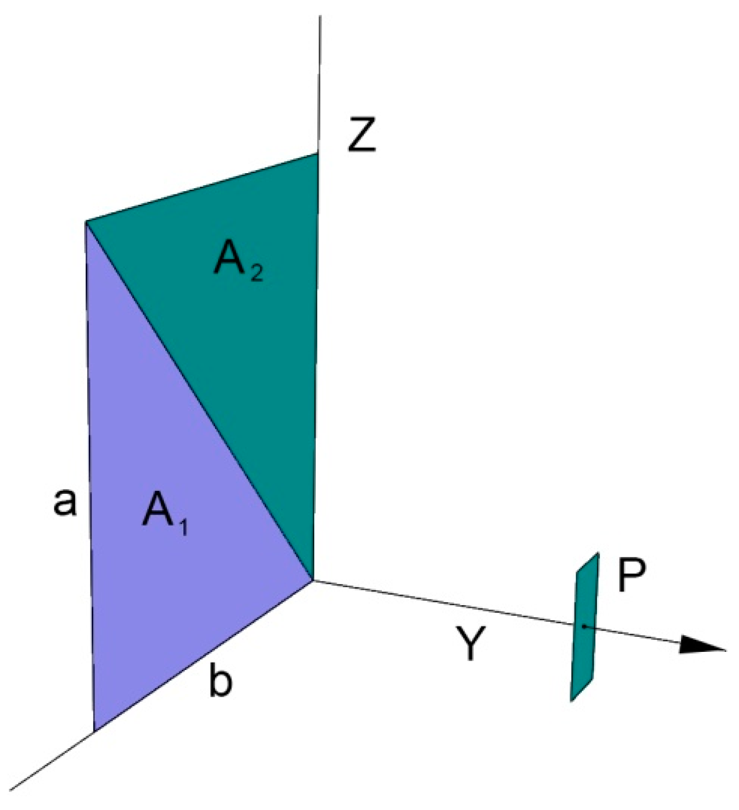
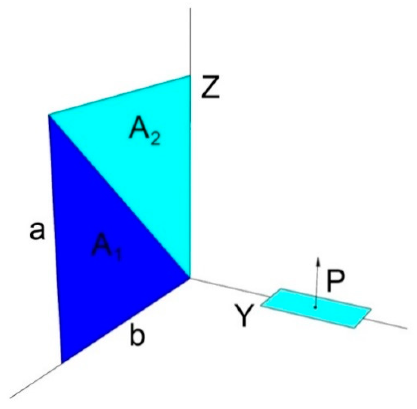
2.1. Triangle
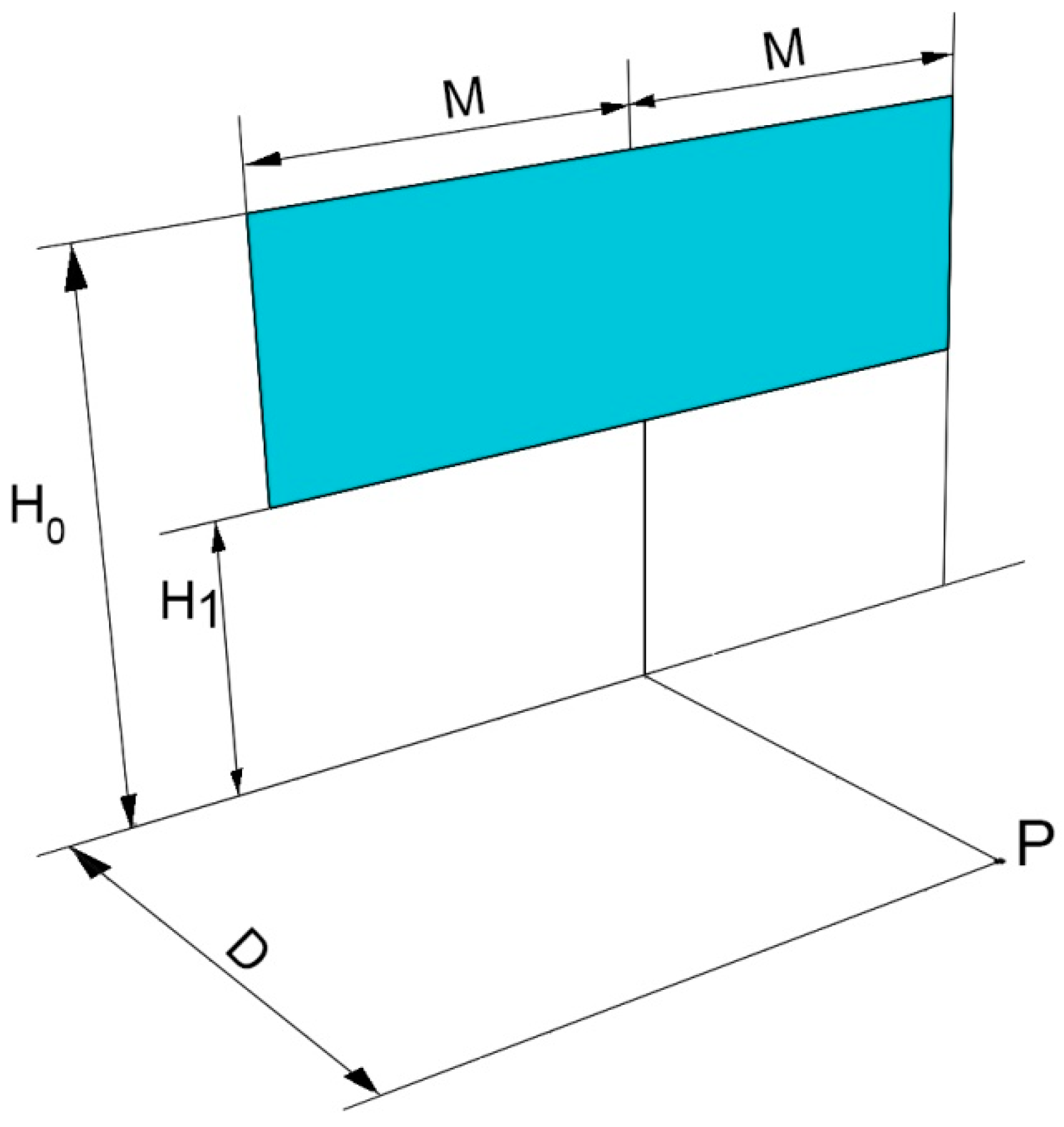
2.2. Rectangle
2.3. Calculations in a Plane Perpendicular to the Figure
2.4. Calculation of Integral Equation for a ‘Rectangle’ Over a Horizontal Square
3. Methodology
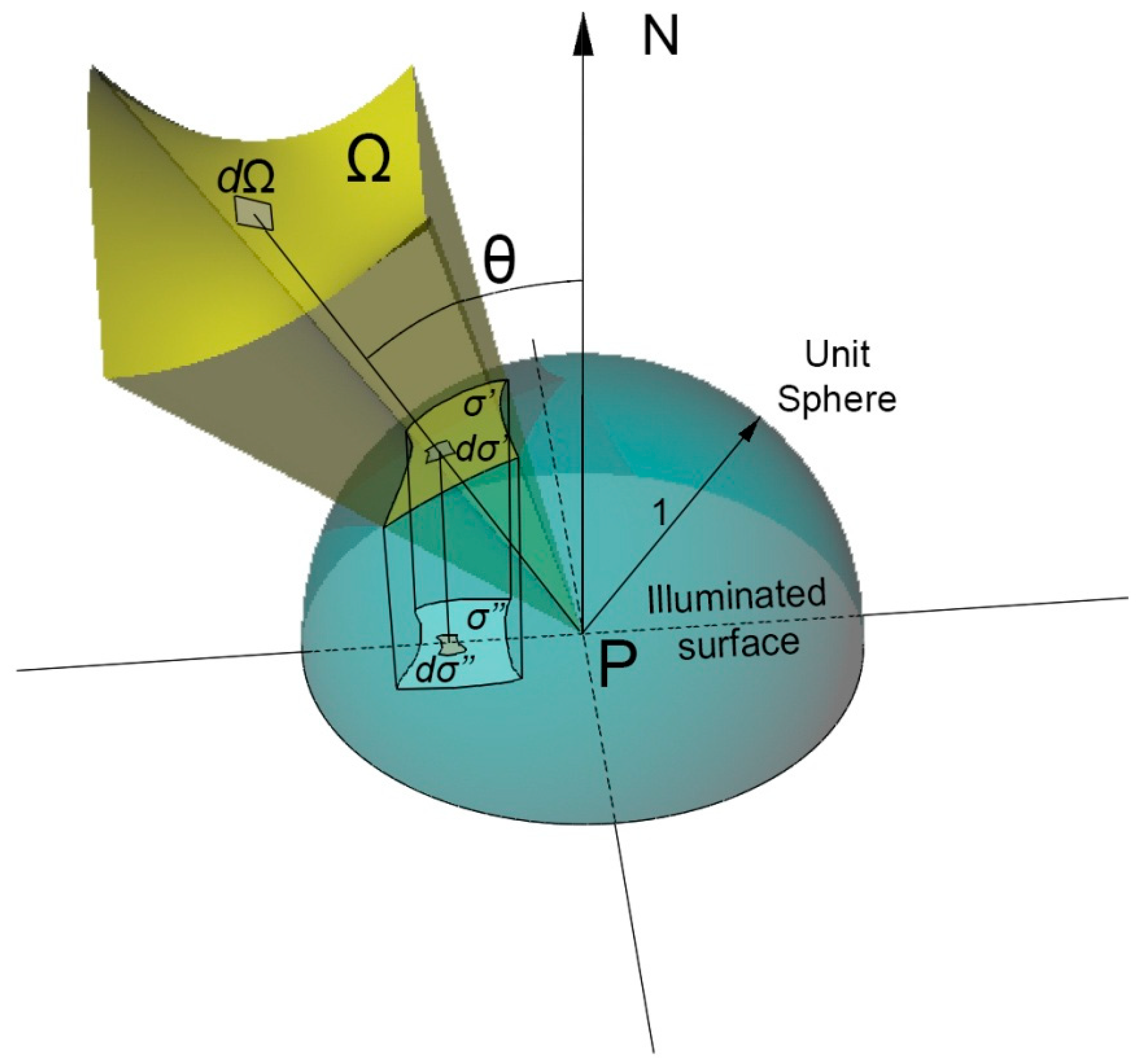
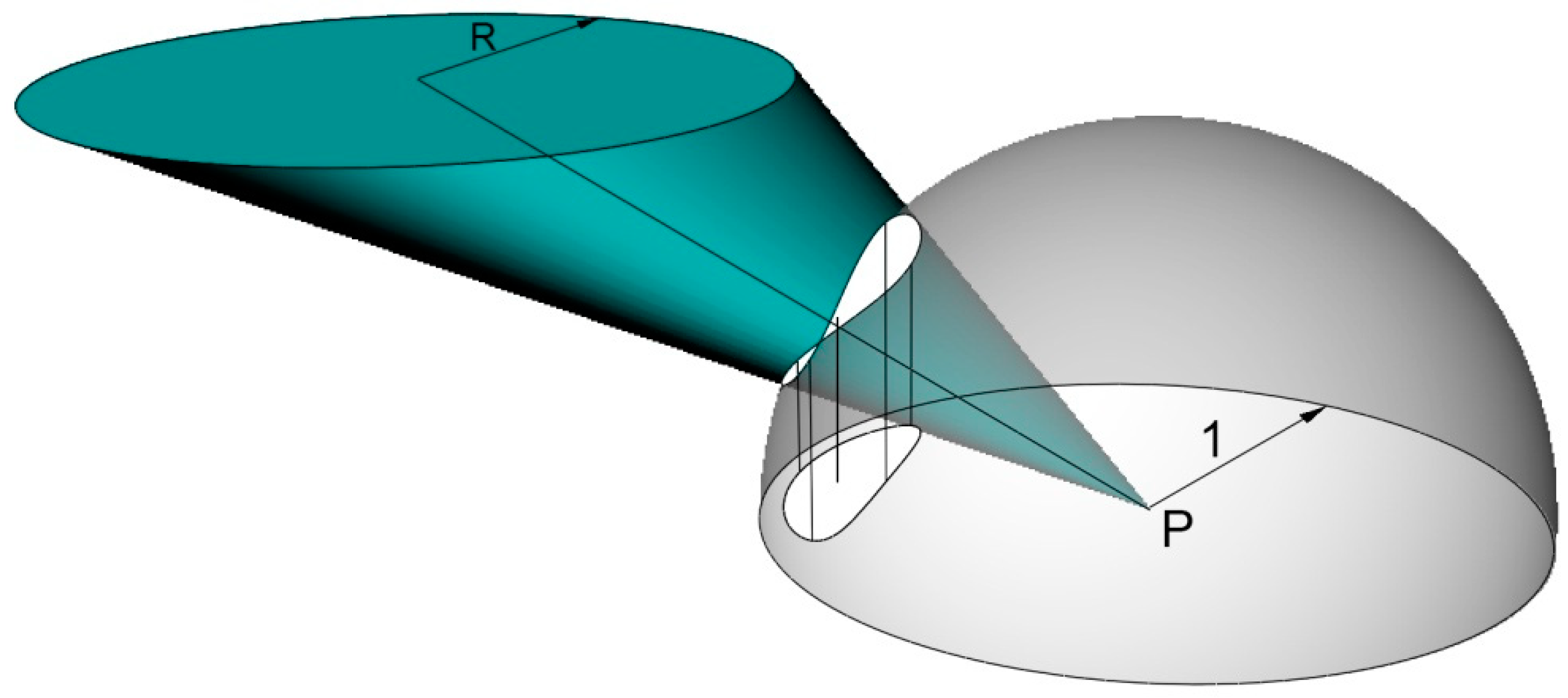
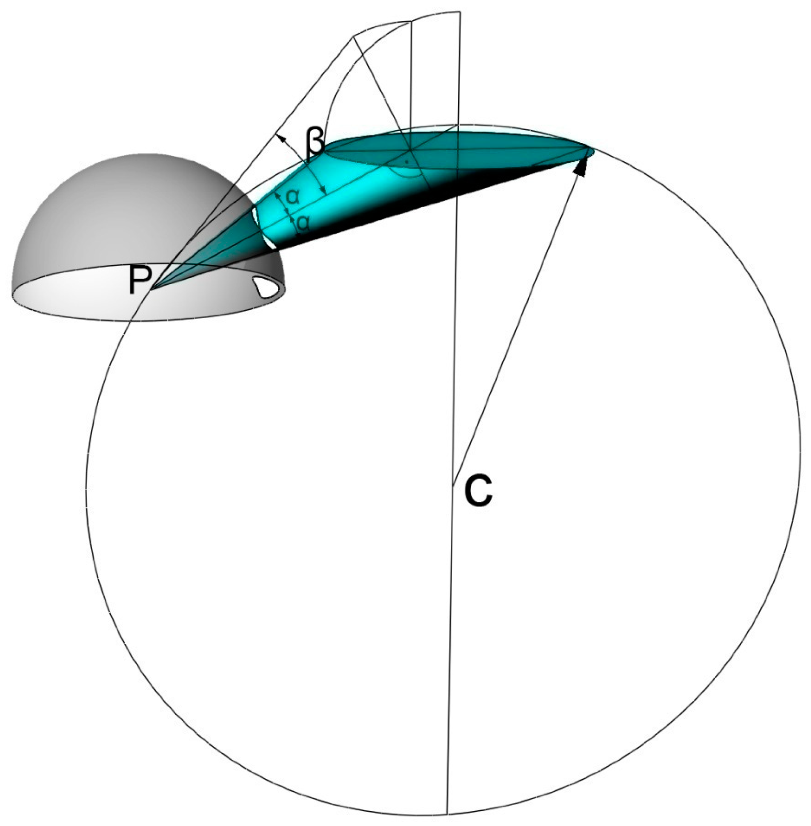
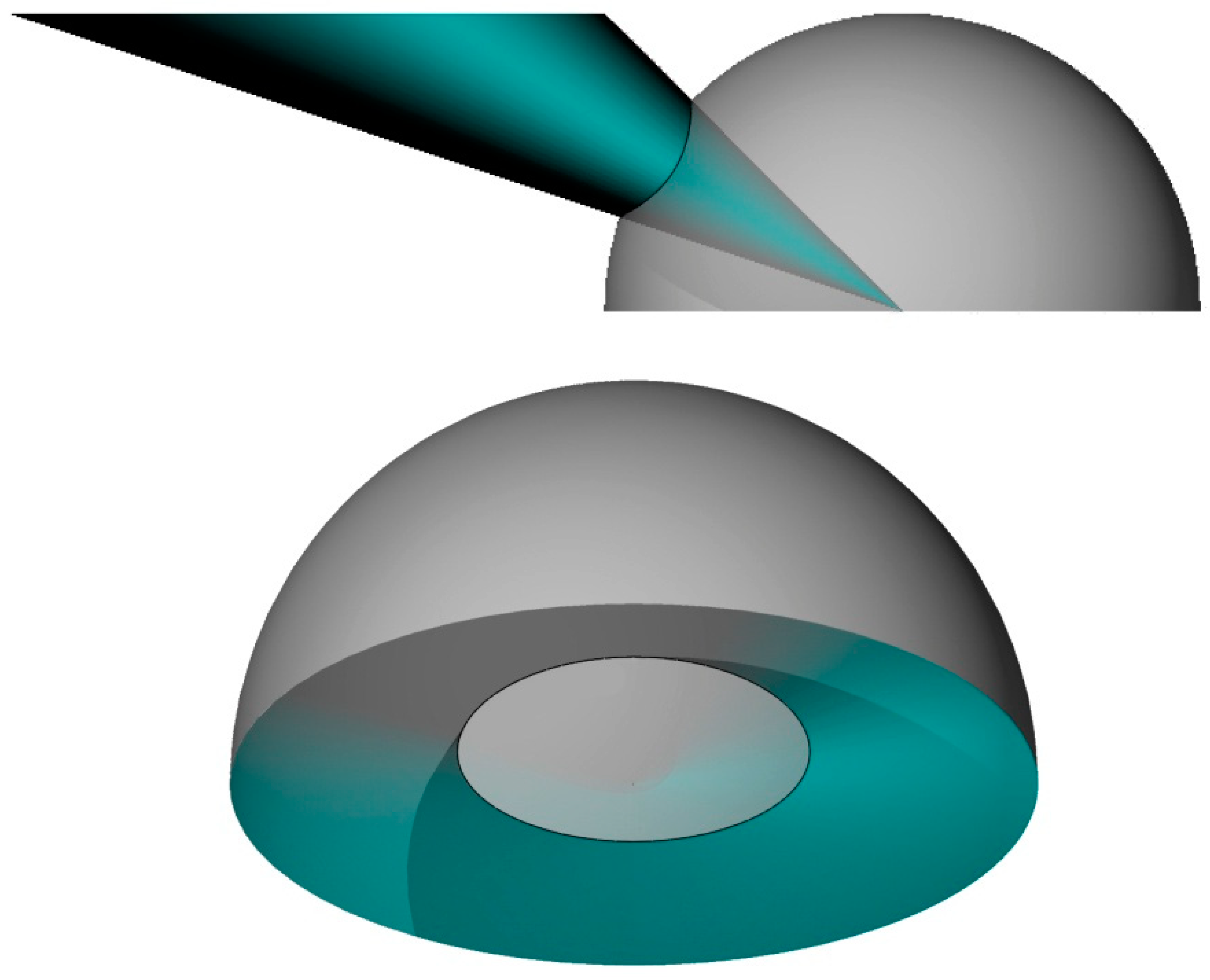
3.1. Solid Angle Projection Law
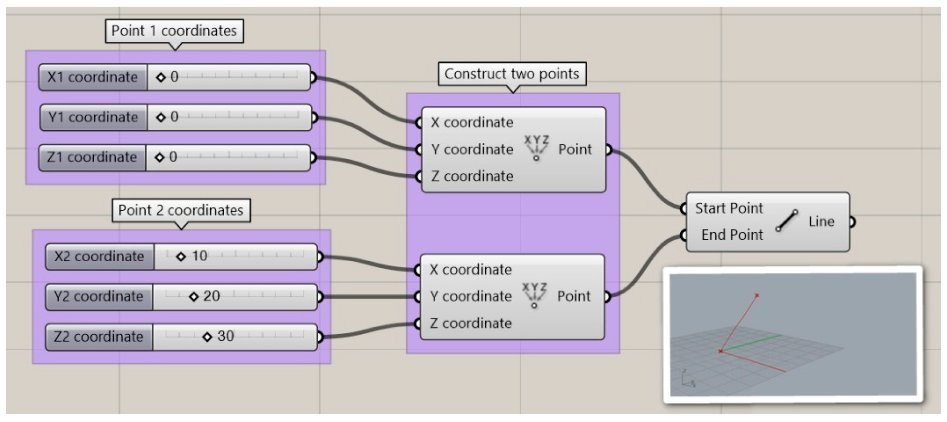
3.2. Algorithms Aided Design
- An algorithm is a well-defined set of properly concise instructions.
- An algorithm demands a defined set of inputs that may or may not come from the output of a previous algorithm.
- An algorithm generates a precise output (Figure 6):
- Finally, an algorithm can produce warnings and error messages through the appropriate editor. If the inputs are not appropriate, e.g., if we enter text instead of numbers, the algorithm will return an error message instead of the expected output, via the appropriate editor [8].
3.3. Calculation by Algorithms Aided Design through Finite Element Method
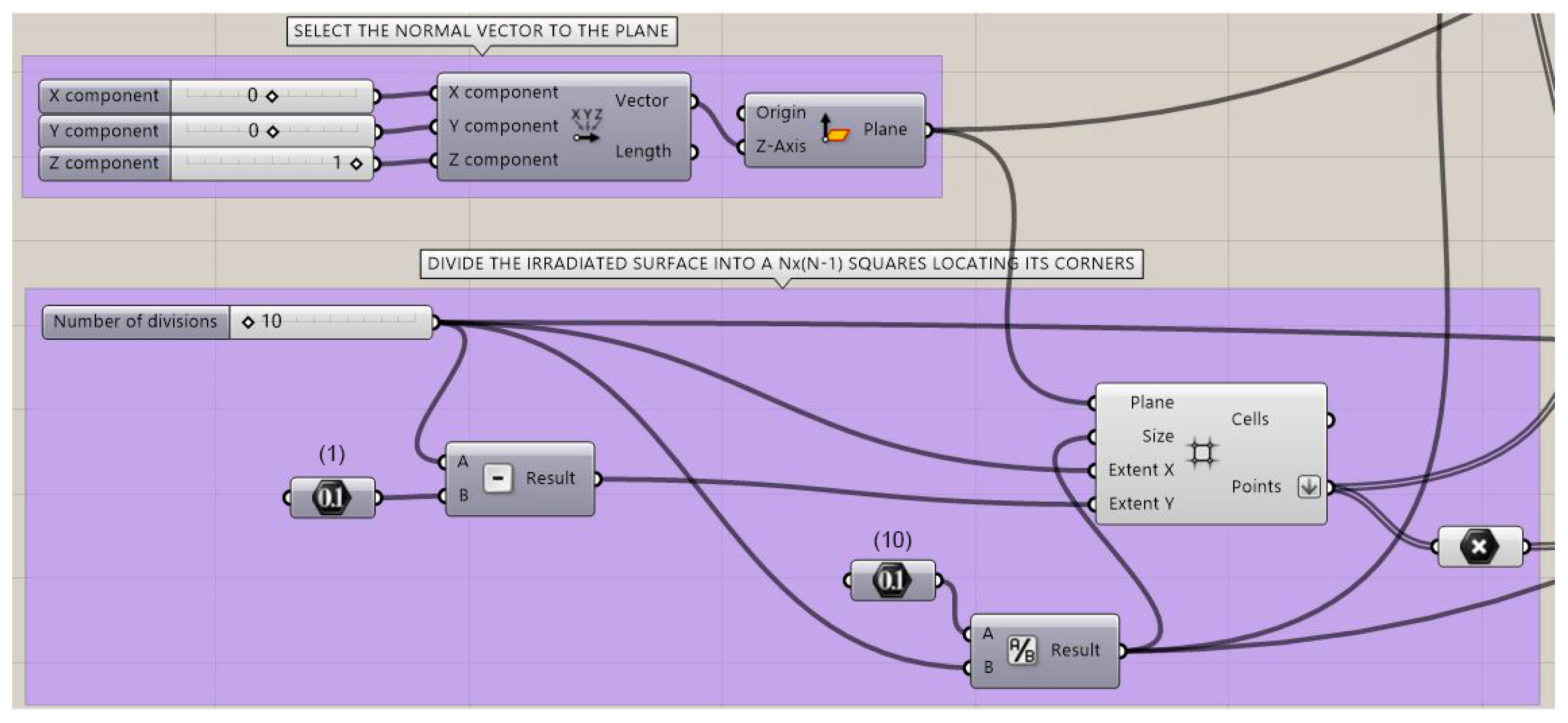
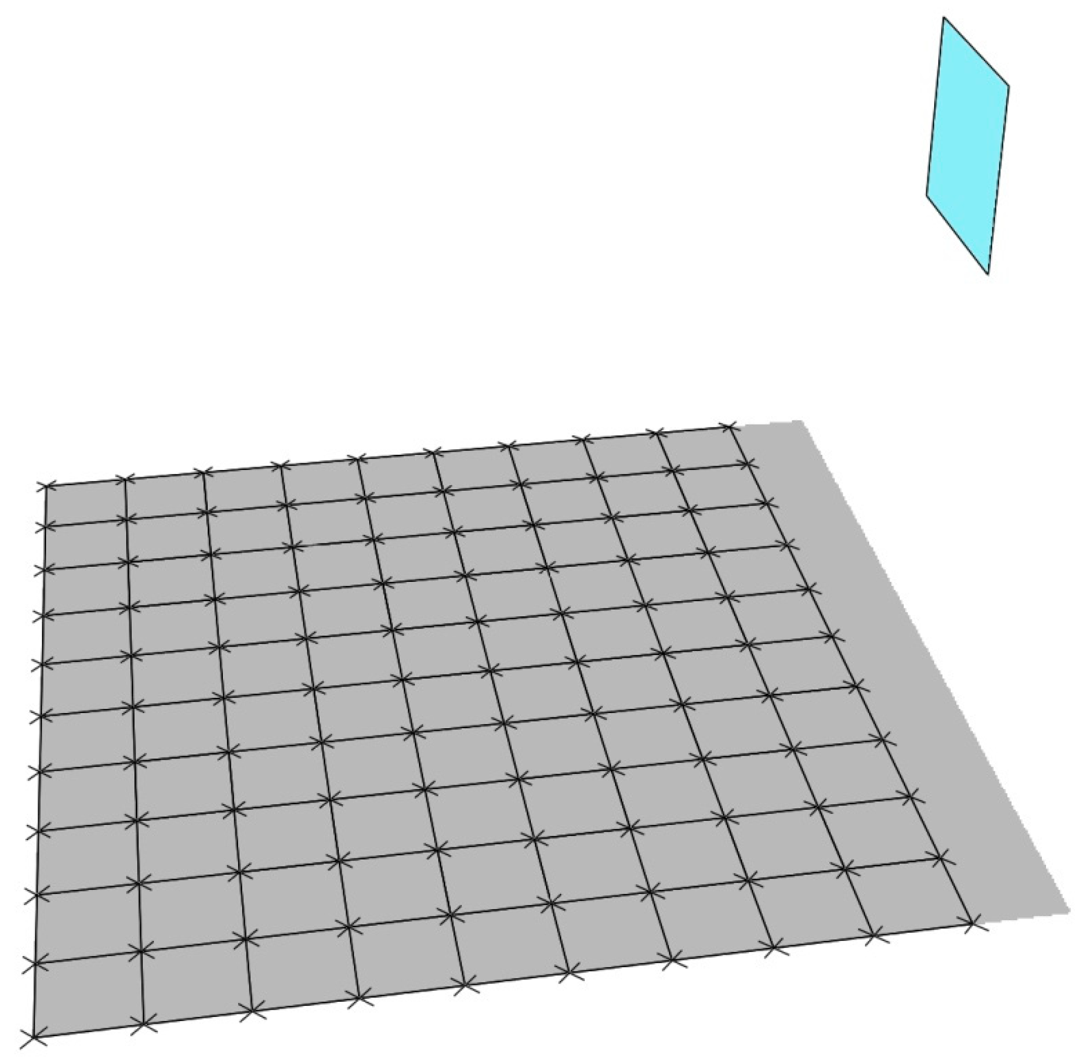
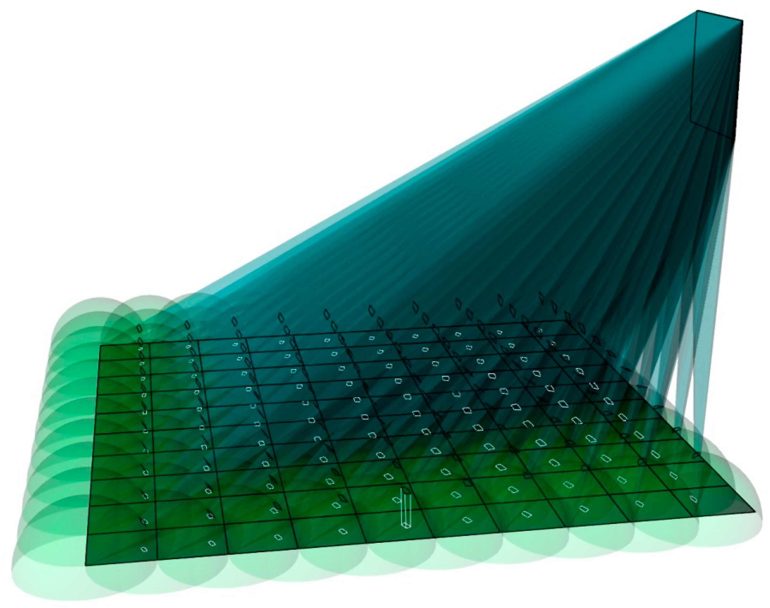
3.3.1. Geometric Definition of Both the Irradiated Surface and the Emitter and, Subsequently, Division of the Irradiated Surface into a Grid of N × (N − 1) Squares, Locating Its Corners
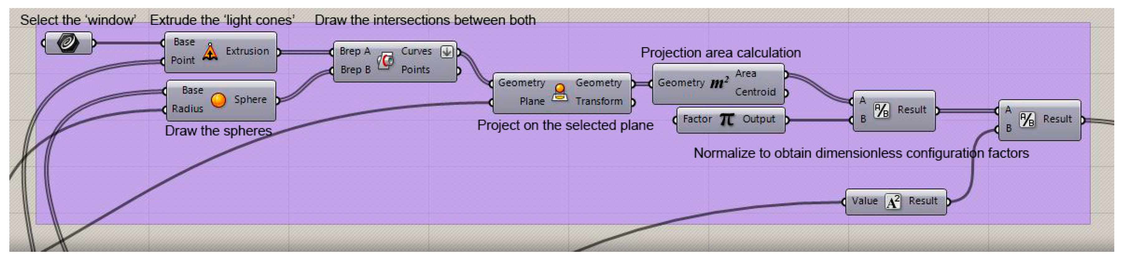
3.3.2. Calculate the Configuration Factors
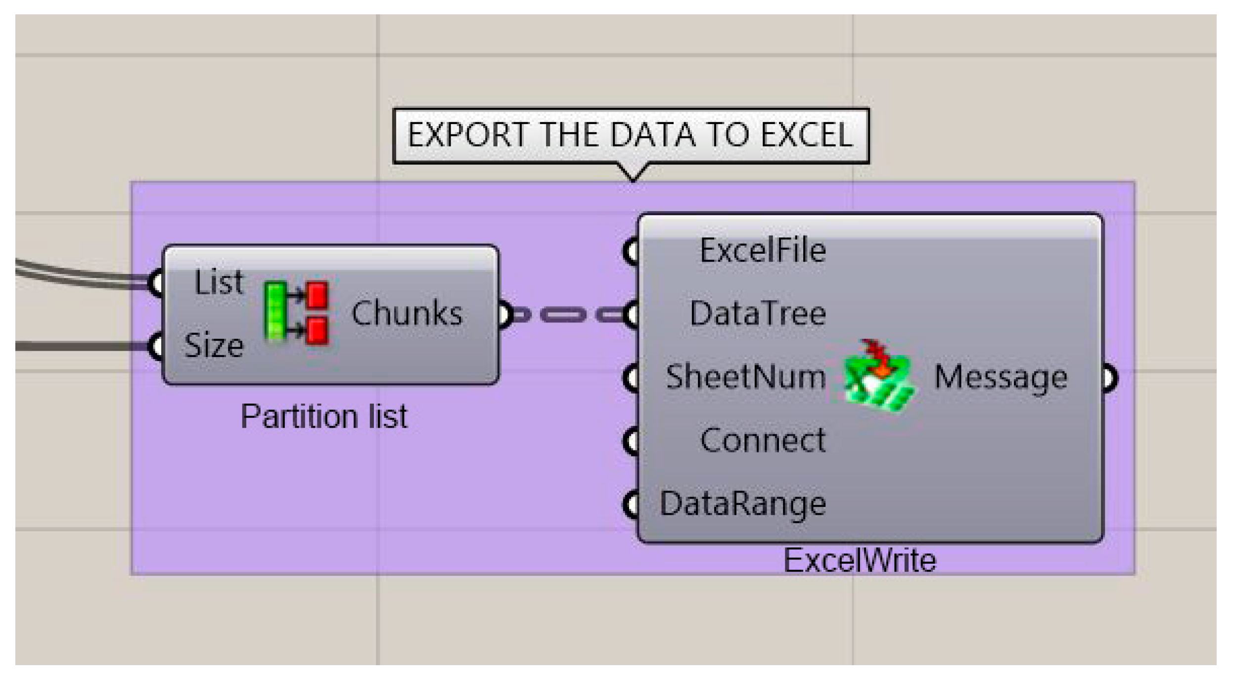
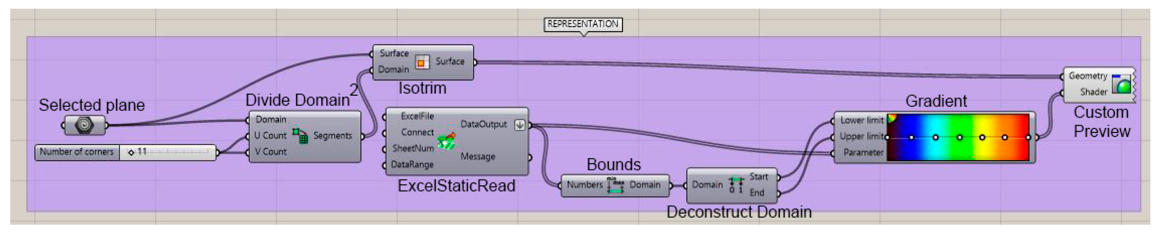
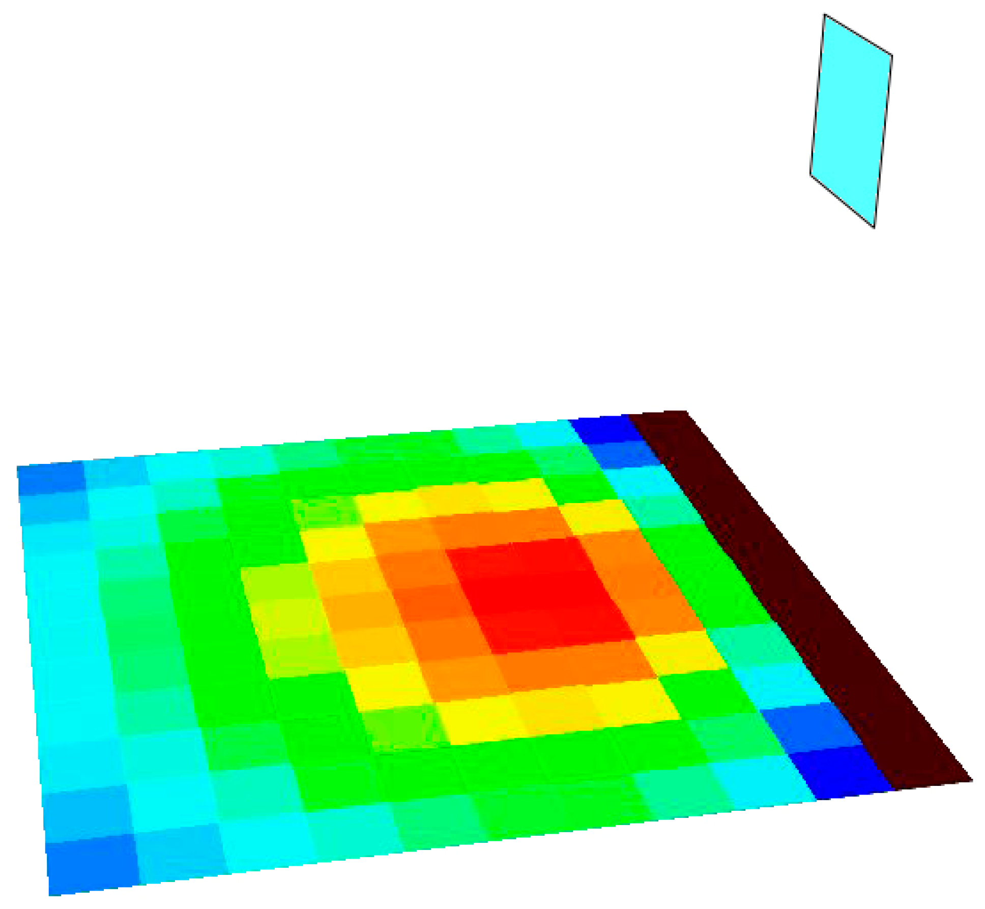
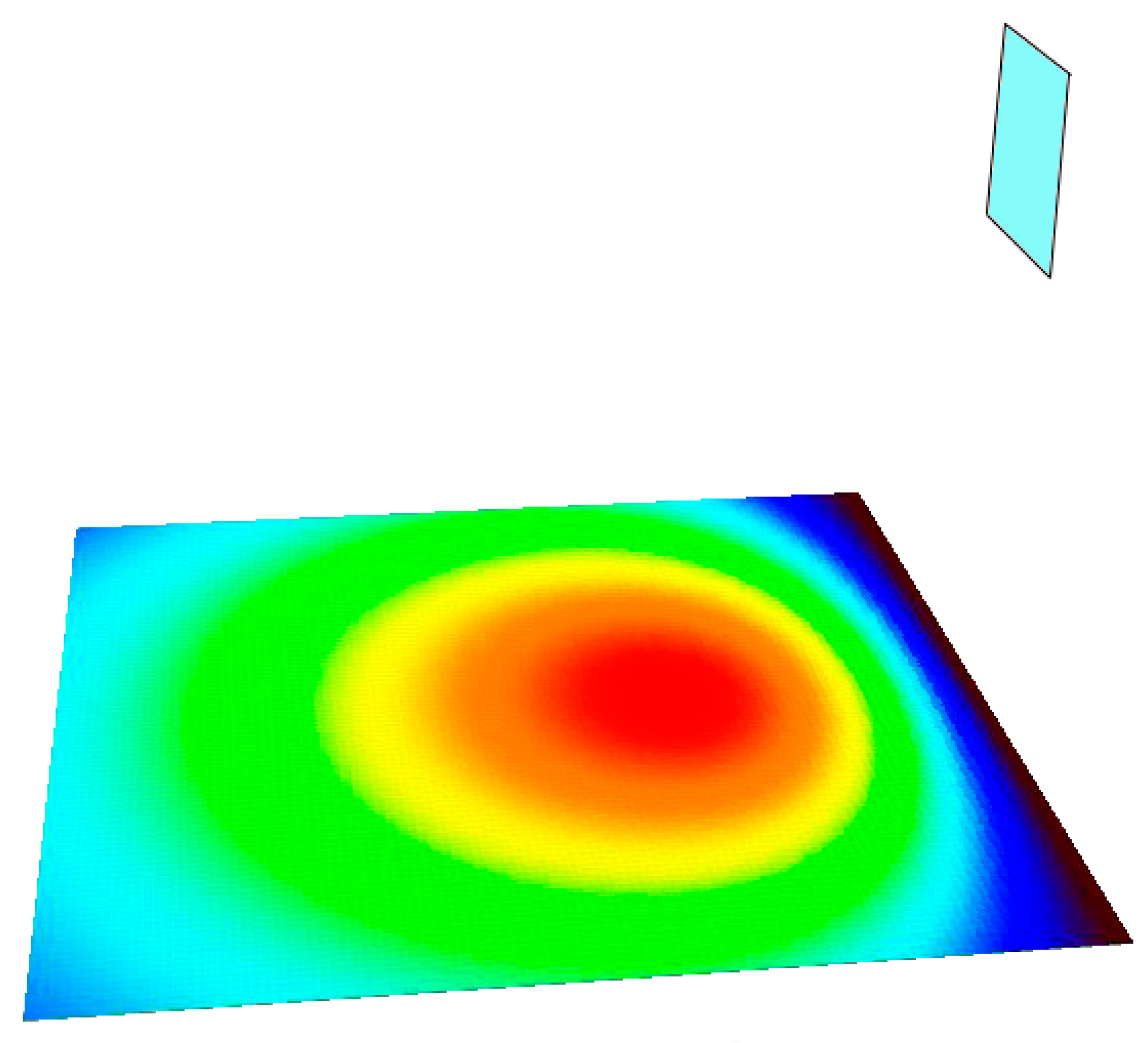
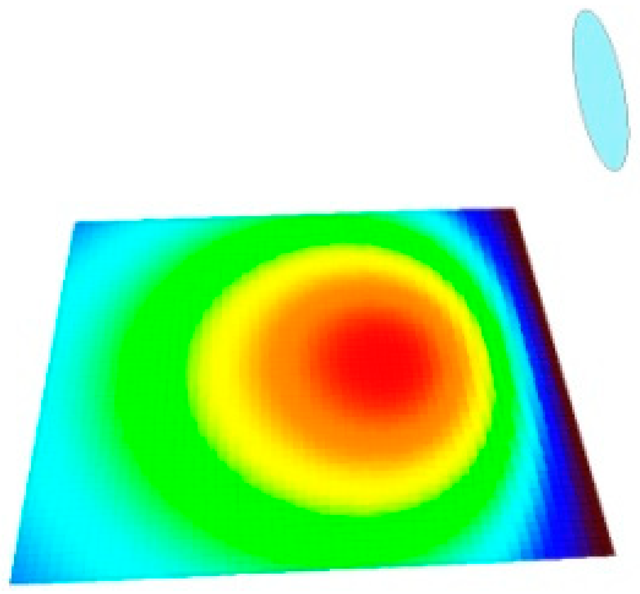
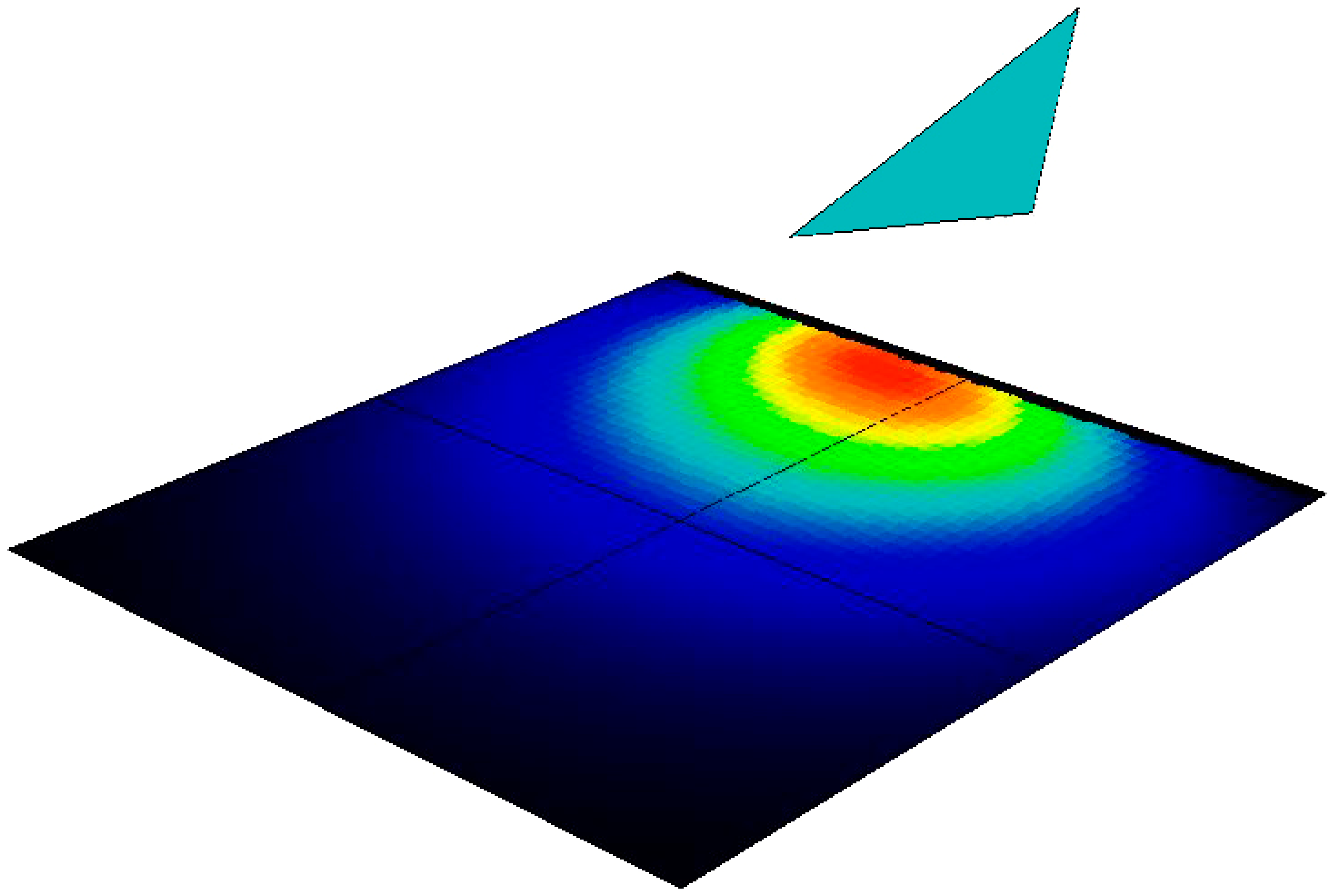
3.3.3. Exporting the Data to Excel and Representing them by Color Maps
3.3.4. Numerical Results
4. Discussion
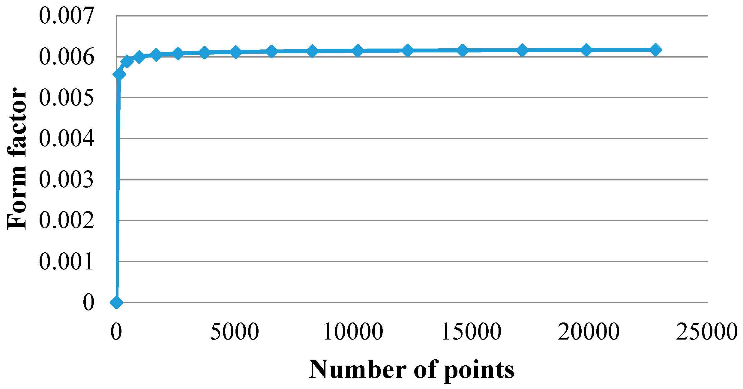
4.1. Convergence
4.2. Versatility of the Method
5. Conclusions and Future Aims
Author Contributions
Funding
Acknowledgments
Conflicts of Interest
Nomenclature
| Fij | Form Factor (surface to surface, dimensionless) |
| fij | Configuration factor (surface to point, dimensionless) |
| Ei, Mi | Emitted Radiant Power (W/m2) |
| Ni | Received Radiant Power (W/m2) |
| ni | Unit Received Radiant Power (point from surface, W/m2) |
| Φi | Radiant flux (W) |
| Li | Emitted Luminance or radiance (W/sr·m2) |
| I | Radiant intensity (W/sr) |
| Ai | Surface area (m2) |
| r | distance (m) |
| θi | angle with the normal (radian) |
| Ω | solid angle (sr) |
Appendix A. Further Details on the Calculations of Basic Configuration Factors
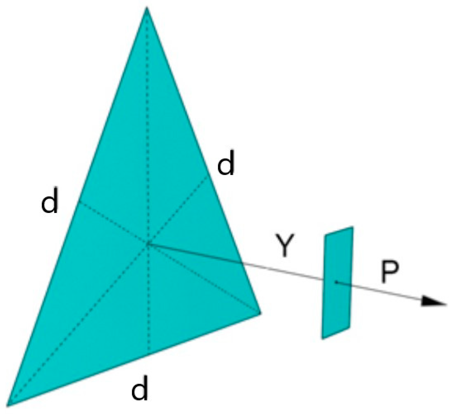
Appendix A.1. Triangles and Shapes Composed of Triangles
Appendix A.2. Rectangle
Appendix A.3. Square
Appendix A.4. Equilateral Triangle

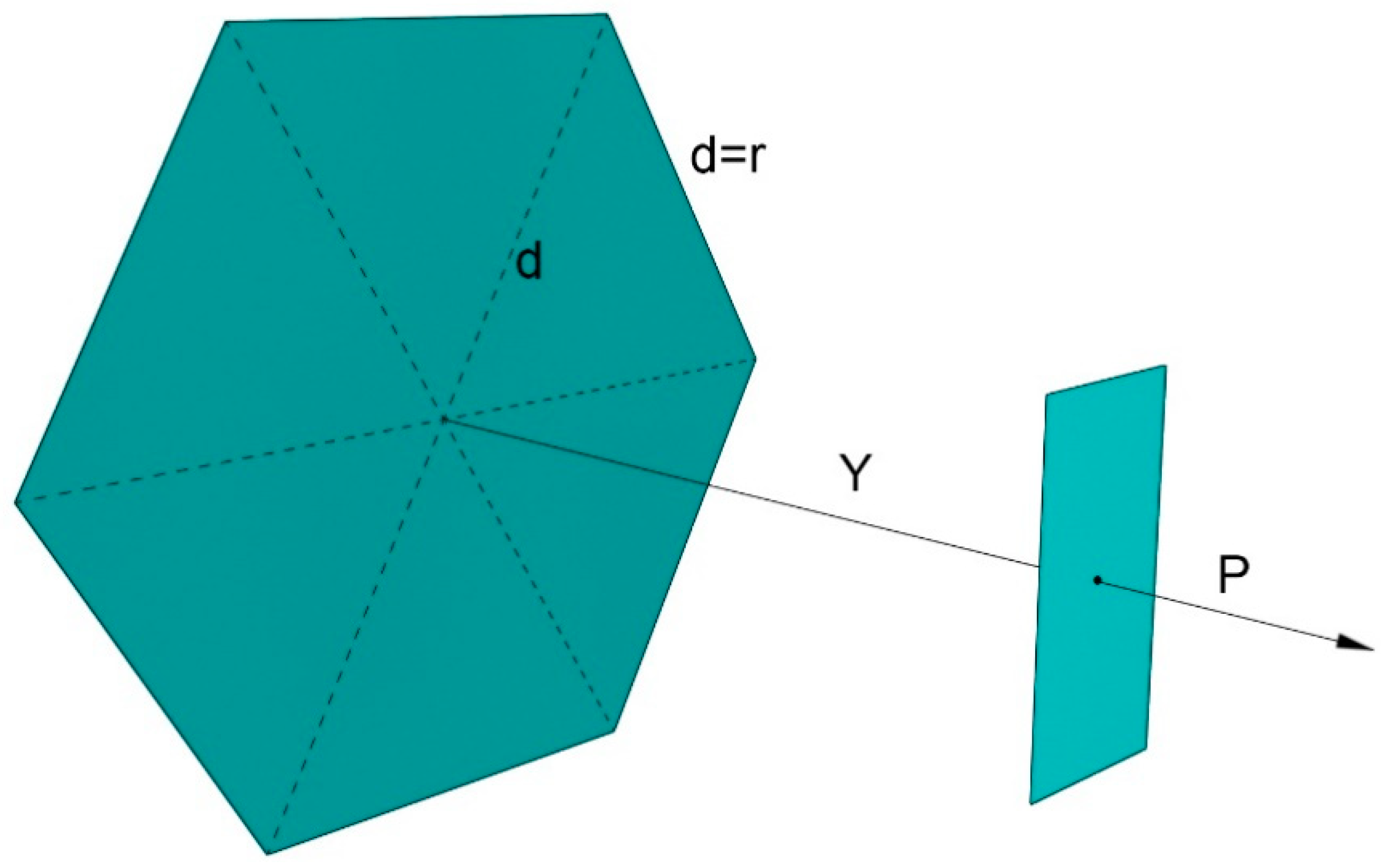
Appendix A.5. Hexagon

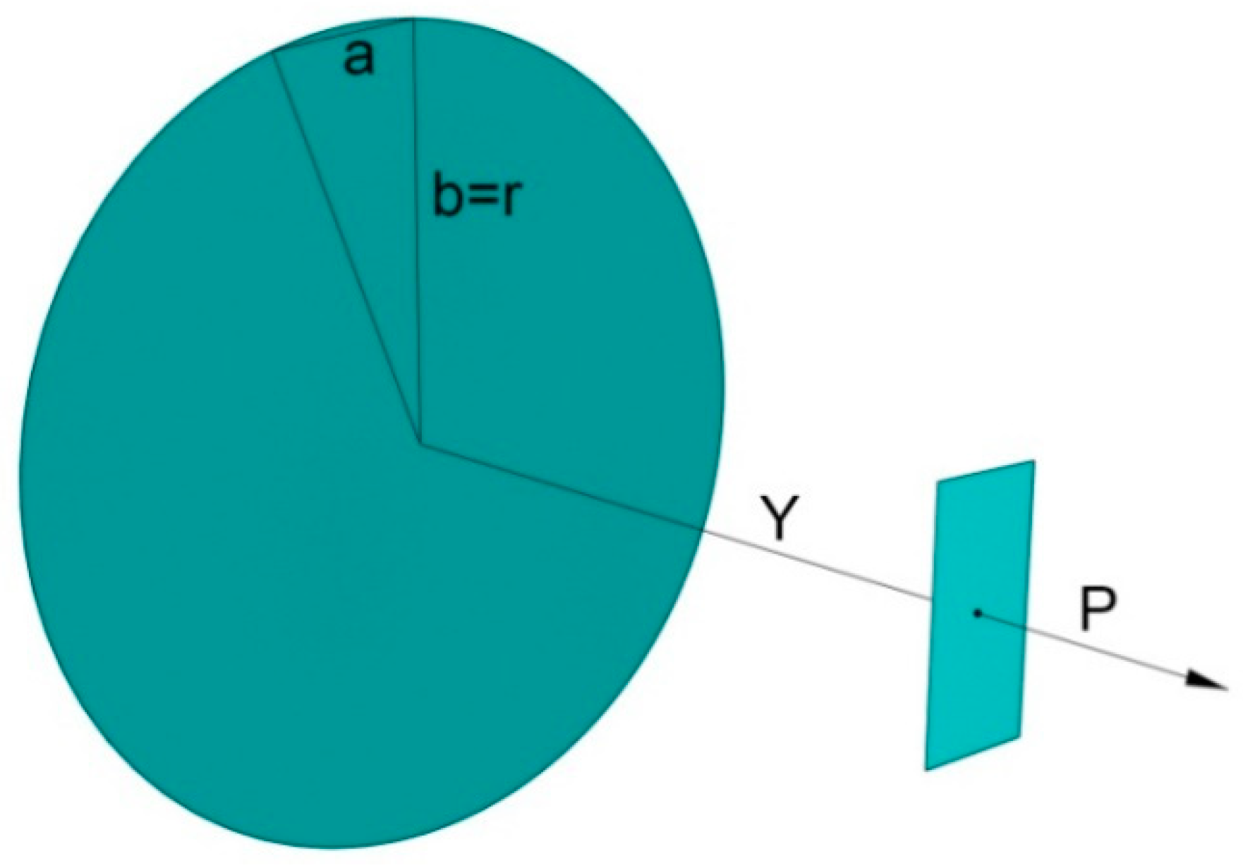
Appendix A.6. Circle

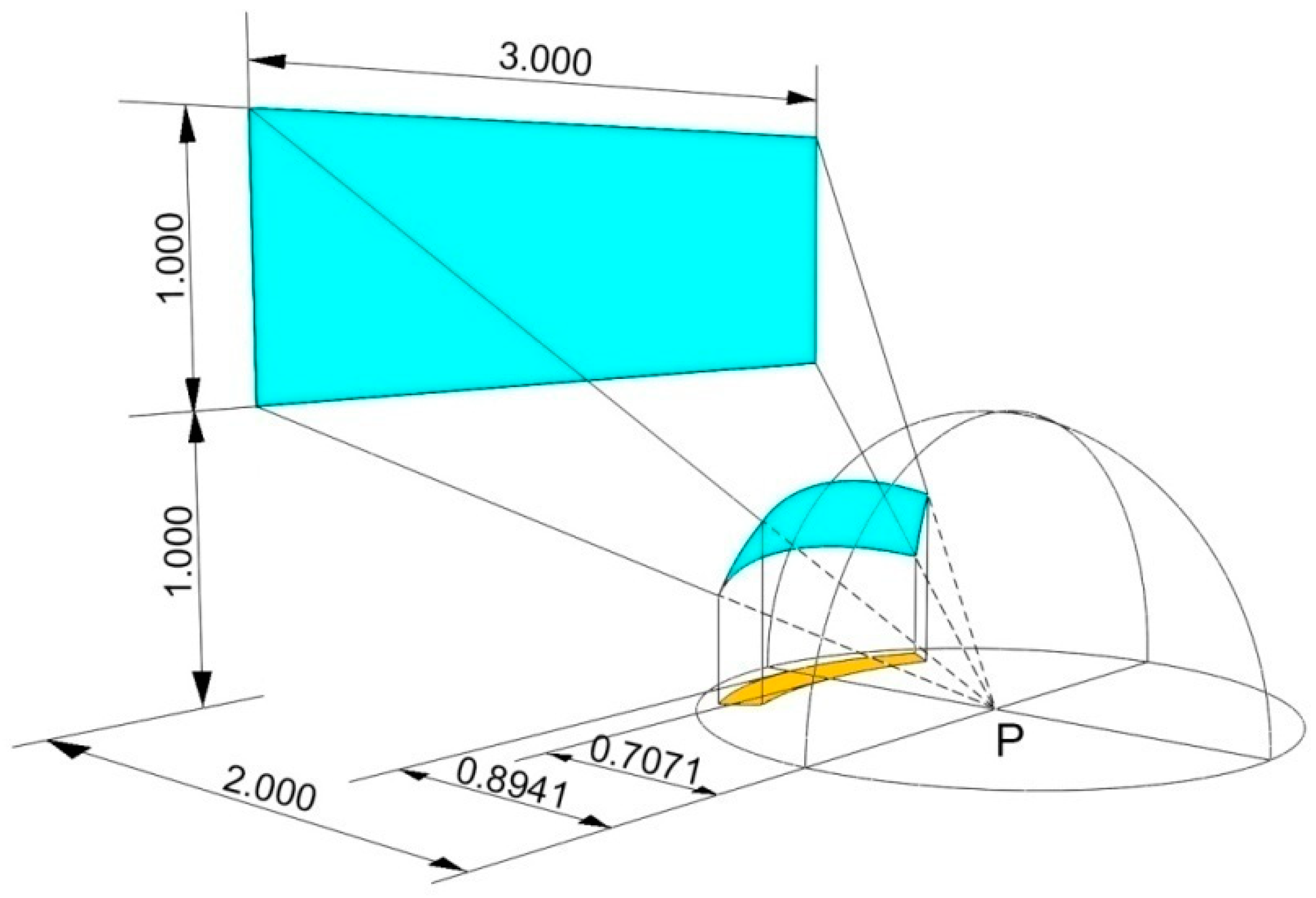
Appendix A.7. Calculations in a Plane Perpendicular to the Figure
Appendix B. Particulars of the Numerical Validation of the Projected Solid-Angle Principle
Numerical Validation for a Rectangle

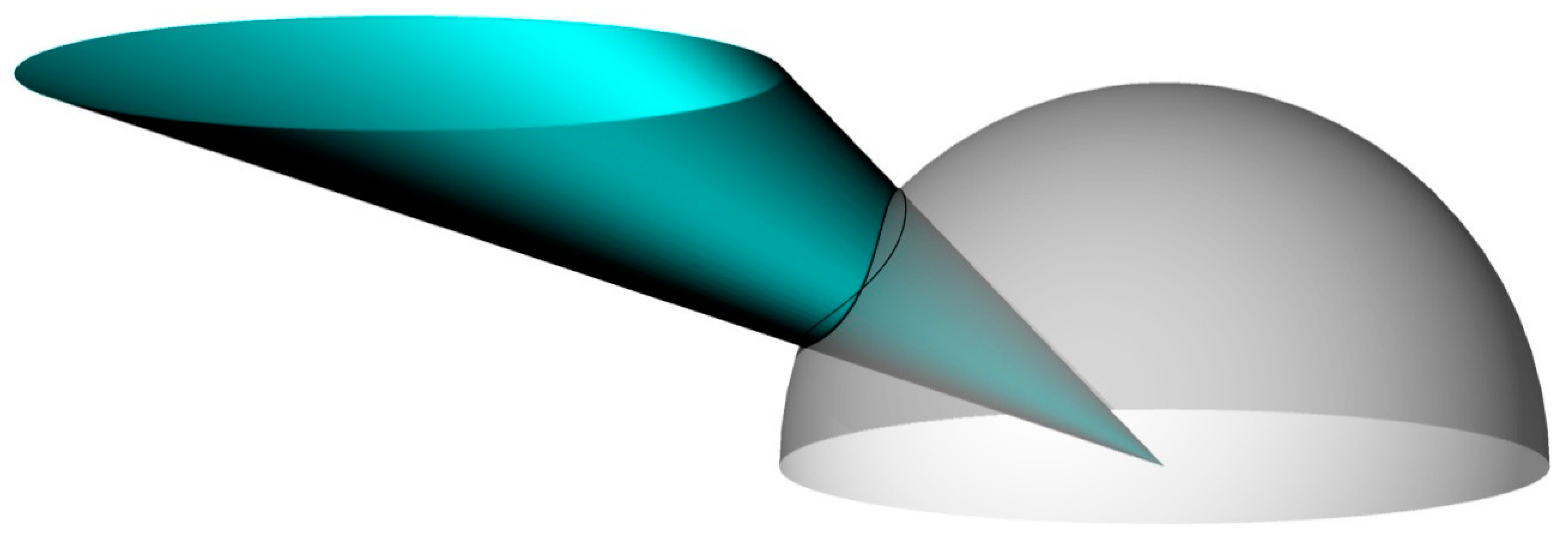
Appendix C. The Recurrent Problem of Circular Emitters


References
- Yamauchi, J. The amount of flux incident to rectangular floor through rectangular windows. Res. Electrotech. Lab. 1929, 250. [Google Scholar]
- Moon, P.H. The Scientific Basis of Illumination Engineering; Dover Publications: New York, NY, USA, 2008. [Google Scholar]
- Moon, P.H.; Spencer, D.E. The Photic Field; The MIT Press: Cambrige, MA, USA, 1981. [Google Scholar]
- Lambert, J.H. Photometry, or, on the Measure and Gradations of Light, Colors, and Shade: Translation from the Latin of Photometria, Sive, De Mensura et Gradibus Luminis, Colorum et Umbrae, with Introductory Monograph and Notes by David L. DiLaura; Illuminating Engineering Society of North America: New York, NY, USA, 2001. [Google Scholar]
- Cabeza-Lainez, J.M. Radiative performance of louvers. Simulation and examples in Asian Architecture. In Proceedings of the 6th International Conference on Indoor Air Quality, Ventilation & Energy Conservation in Buildings (IAQVEC), Sendai, Japan, 28–31 October 2007; Volume 3, ISBN 978-4-86163-072-9. C3025\4762E. [Google Scholar]
- Cabeza-Lainez, J.M. Fundamentos de Transferencia Radiante Luminosa o la Verdadera Naturaleza del Factor de Forma y sus Modelos de Cálculo; Netbiblio: Seville, Spain, 2010. [Google Scholar]
- Cabeza-Lainez, J.M.; Pulido-Arcas, J.A. New configuration factors for curved surfaces. J. Quant. Spectrosc. Radiat. Transf. 2013, 117, 71–80. [Google Scholar] [CrossRef]
- Tedeschi, A. AAD_Algorithms-Aided Design. Parametric Strategies Using Grasshopper®; Le Penseur Publisher: Potenza, Italy, 2014; pp. 22–23. [Google Scholar]
- Fock, V.A. Zur Berechnung der Beleuchtungsstärke. Z. Phys. 1924, 28, 102–113. [Google Scholar] [CrossRef]
- Sasaki, K.; Sznajder, M. Analytical view factor solutions of a spherical cap from an infinitesimal surface. Int. J. Heat Mass Transf. 2020, 163, 120477. [Google Scholar] [CrossRef]
- Salguero Andujar, F.; Rodriguez-Cunill, I.; Cabeza-Lainez, J.M. The problem of lighting in underground domes, vaults, and tunnel-like structures of antiquity; an application to the sustainability of prominent Asian heritage (India, Korea, China). Sustainability 2019, 11, 5865. [Google Scholar] [CrossRef]
- Gershun, A. The Light Field (translated by P. Moon and G. Timoshenko). J. Math. Phys. 1939, 18, 51–151. [Google Scholar] [CrossRef]


| Distance in the X-Axis to the Rectangle’s Plane (m) | ||||||||||||
|---|---|---|---|---|---|---|---|---|---|---|---|---|
| Distance in the Y-axis to the Rectangles Plane (m) | 0 | 1 | 2 | 3 | 4 | 5 | 6 | 7 | 8 | 9 | 10 | |
| Dimensionless Configuration Factor f12 (i.e., Divided by π) | ||||||||||||
| 0 | 0.00000 | 0.00000 | 0.00000 | 0.00000 | 0.00000 | 0.00000 | 0.00000 | 0.00000 | 0.00000 | 0.00000 | 0.00000 | |
| 1 | 0.00203 | 0.00279 | 0.00371 | 0.00469 | 0.00546 | 0.00577 | 0.00546 | 0.00469 | 0.00371 | 0.00279 | 0.00203 | |
| 2 | 0.00368 | 0.00497 | 0.00650 | 0.00807 | 0.00930 | 0.00977 | 0.00930 | 0.00807 | 0.00650 | 0.00497 | 0.00368 | |
| 3 | 0.00473 | 0.00624 | 0.00796 | 0.00966 | 0.01096 | 0.01144 | 0.01096 | 0.00966 | 0.00796 | 0.00624 | 0.00473 | |
| 4 | 0.00519 | 0.00665 | 0.00825 | 0.00977 | 0.01090 | 0.0132 | 0.01090 | 0.00977 | 0.00825 | 0.00665 | 0.00519 | |
| 5 | 0.00517 | 0.00644 | 0.00778 | 0.00901 | 0.00989 | 0.01021 | 0.00989 | 0.00901 | 0.00778 | 0.00644 | 0.00517 | |
| 6 | 0.00486 | 0.00590 | 0.00695 | 0.00788 | 0.00852 | 0.00876 | 0.00852 | 0.00788 | 0.00695 | 0.00590 | 0.00486 | |
| 7 | 0.00440 | 0.00521 | 0.00600 | 0.00668 | 0.00715 | 0.00732 | 0.00715 | 0.00668 | 0.00600 | 0.00521 | 0.00440 | |
| 8 | 0.00389 | 0.00451 | 0.00510 | 0.00559 | 0.00592 | 0.00604 | 0.00592 | 0.00559 | 0.00510 | 0.00451 | 0.00389 | |
| 9 | 0.00339 | 0.00385 | 0.00429 | 0.00464 | 0.00488 | 0.00496 | 0.00488 | 0.00464 | 0.00429 | 0.00385 | 0.00339 | |
| 10 | 0.00293 | 0.00328 | 0.00360 | 0.00386 | 0.00402 | 0.00408 | 0.00402 | 0.00386 | 0.00360 | 0.00328 | 0.00293 | |
| Distance in the X-Axis to the Rectangle’s Plane (m) | |||||||
|---|---|---|---|---|---|---|---|
| Distance in the Y-axis to the Rectangle-s Plane (m) | 5 | 6 | 7 | 8 | 9 | 10 | |
| Dimensionless Configuration Factor f12 | |||||||
| 0 | 0.00000000 | 0.00000000 | 0.00000000 | 0.00000000 | 0.00000000 | 0.00000000 | |
| 1 | 0.005765 | 0.00546298 | 0.00468552 | 0.00371248 | 0.00278731 | 0.00202982 | |
| 2 | 0.00976818 | 0.00929669 | 0.00806846 | 0.00649857 | 0.00496683 | 0.00367902 | |
| 3 | 0.01144492 | 0.01095576 | 0.00966096 | 0.00795806 | 0.00623622 | 0.00473341 | |
| 4 | 0.01131701 | 0.0108993 | 0.00977478 | 0.00824998 | 0.00664699 | 0.00518805 | |
| 5 | 0.01020997 | 0.00988871 | 0.00901007 | 0.00778368 | 0.00644494 | 0.0051747 | |
| 6 | 0.00875831 | 0.00852443 | 0.00787588 | 0.0069471 | 0.00589812 | 0.00486368 | |
| 7 | 0.0073163 | 0.00715037 | 0.0066848 | 0.00600327 | 0.0052104 | 0.00440123 | |
| 8 | 0.00603659 | 0.00591986 | 0.00558912 | 0.00509595 | 0.00450753 | 0.00388887 | |
| 9 | 0.00496121 | 0.00487895 | 0.004644 | 0.00428824 | 0.00385462 | 0.00338694 | |
| 10 | 0.00408173 | 0.00402333 | 0.00385542 | 0.00359789 | 0.00327834 | 0.00292612 | |
| Distance in the X-Axis to the Triangle’s Plane (m) | ||||||||||||
|---|---|---|---|---|---|---|---|---|---|---|---|---|
| Distance in the Y-axis to the Triangles Plane (m) | 0 | 1 | 2 | 3 | 4 | 5 | 6 | 7 | 8 | 9 | 10 | |
| Dimensionless Configuration Factor f12 (i.e., Divided by π) | ||||||||||||
| 0 | 0.00000 | 0.00000 | 0.00000 | 0.00000 | 0.00000 | 0.00000 | 0.00000 | 0.00000 | 0.00000 | 0.00000 | 0.00000 | |
| 1 | 0.00329 | 0.00593 | 0.01103 | 0.02039 | 0.03471 | 0.04974 | 0.05761 | 0.05139 | 0.03030 | 0.01256 | 0.005371 | |
| 2 | 0.00554 | 0.00942 | 0.01614 | 0.02677 | 0.04031 | 0.05151 | 0.05363 | 0.04433 | 0.02858 | 0.01539 | 0.00799 | |
| 3 | 0.00642 | 0.01014 | 0.01581 | 0.02349 | 0.03169 | 0.03715 | 0.03682 | 0.03064 | 0.02171 | 0.01371 | 0.00825 | |
| 4 | 0.00627 | 0.00921 | 0.01318 | 0.01789 | 0.02229 | 0.02476 | 0.02415 | 0.02067 | 0.01578 | 0.01106 | 0.00740 | |
| 5 | 0.00559 | 0.00769 | 0.01027 | 0.01303 | 0.01535 | 0.01650 | 0.01604 | 0.01413 | 0.01141 | 0.00862 | 0.00623 | |
| 6 | 0.00474 | 0.00619 | 0.00782 | 0.00943 | 0.01069 | 0.01126 | 0.01097 | 0.00989 | 0.00833 | 0.00664 | 0.00509 | |
| 7 | 0.00392 | 0.00490 | 0.00593 | 0.00689 | 0.00761 | 0.00791 | 0.00773 | 0.00710 | 0.00618 | 0.00513 | 0.00411 | |
| 8 | 0.00321 | 0.00387 | 0.00453 | 0.00513 | 0.00554 | 0.00572 | 0.00560 | 0.00552 | 0.00465 | 0.00399 | 0.00332 | |
| 9 | 0.00262 | 0.00307 | 0.00351 | 0.00388 | 0.00414 | 0.00424 | 0.00416 | 0.00393 | 0.00357 | 0.00314 | 0.00268 | |
| 10 | 0.00214 | 0.00246 | 0.00275 | 0.00299 | 0.00315 | 0.00322 | 0.00316 | 0.00302 | 0.00278 | 0.00249 | 0.00218 | |
Publisher’s Note: MDPI stays neutral with regard to jurisdictional claims in published maps and institutional affiliations. |
© 2020 by the authors. Licensee MDPI, Basel, Switzerland. This article is an open access article distributed under the terms and conditions of the Creative Commons Attribution (CC BY) license (http://creativecommons.org/licenses/by/4.0/).
Share and Cite
Salguero-Andújar, F.; Cabeza-Lainez, J.-M. New Computational Geometry Methods Applied to Solve Complex Problems of Radiative Transfer. Mathematics 2020, 8, 2176. https://doi.org/10.3390/math8122176
Salguero-Andújar F, Cabeza-Lainez J-M. New Computational Geometry Methods Applied to Solve Complex Problems of Radiative Transfer. Mathematics. 2020; 8(12):2176. https://doi.org/10.3390/math8122176
Chicago/Turabian StyleSalguero-Andújar, Francisco, and Joseph-Maria Cabeza-Lainez. 2020. "New Computational Geometry Methods Applied to Solve Complex Problems of Radiative Transfer" Mathematics 8, no. 12: 2176. https://doi.org/10.3390/math8122176
APA StyleSalguero-Andújar, F., & Cabeza-Lainez, J.-M. (2020). New Computational Geometry Methods Applied to Solve Complex Problems of Radiative Transfer. Mathematics, 8(12), 2176. https://doi.org/10.3390/math8122176