Some Escape Time Results for General Complex Polynomials and Biomorphs Generation by a New Iteration Process

Abstract

Biomorphs are graphic objects with very interesting shapes resembling unicellular and microbial organisms such as bacteria. They have applications in different fields like medical science, art, painting, engineering and the textile industry. In this paper, we present for the first time escape criterion results for general complex polynomials containing quadratic, cubic and higher order polynomials. We do so by using a more general iteration method also used for the first time in this field. This also generalizes some previous results. Then, biomorphs are generated using an algorithm whose pseudocode is included. A visualization of the biomorphs for certain polynomials is presented and their graphical behaviour with respect to variation of parameters is examined.

1. Introduction

Historically, British writer Geoffrey Grigson in 1935 coined the term biomorphism in the context of art [1]. Biomorphs are also used in painting [2], architecture [3,4] and industrial design [5,6]. Biomorph may be defined as a painted, drawn, or sculptured free form or design suggestive in shape of a living organism, especially an ameba or protozoan. The concept of fractal generations has a rich history in computer graphics. In 1918, Gaston Julia introduced the Julia set using a simple iterative process to generate interesting fractals. Interest in this concept has grown significantly due to the visual beauty, complexity and self similarity of the Julia sets; see for instance [7,8,9,10,11]. In 1975, Benoit Mandelbrot [12] extended the work of Gaston Julia and introduced a new set of connected Julia sets called Mandelbrot set. The Mandelbrot and Julia sets have been studied for quadratic [9,11,13,14], cubic [9,14,15,16,17], and higher degree polynomials [18] under Picard orbit, which is a one-step iteration process.

Recently, Rani and Kumar [19,20] studied a one-step Mann iteration process for generating Julia and Mandelbrot sets for a class of n degree complex polynomials. Their work was further extended by Chauhan et al. [21] by studying a two-step Ishikawa iteration for generating relative superior Julia and Mandelbrot sets. Moreover, Chauhan et al. [22] studied the two-step Ishikawa iteration process for non-integer values polynomials for generating relative superior Julia and Mandelbrot sets. Furthermore, Ashish and Rani [23] investigated three-step Noor iterations for generating Julia and Mandelbrot sets. Very recently, many others have proposed other forms of iterations for generating different Julia and Mandelbrot sets; see, for instance, [24] and references therein.

In 1986, Pickover introduced a modification of the Julia sets called biomorphs [25]. Though the biomorphs were accidentally found by Pickover, they have found applications in biology and art (see [26,27,28]). We note that there are very few results on iterative methods for generating biomorphs in the literature. In 2016, Gdawiec et al. [29] introduced a new set of biomorphs by using Pickover algorithm with Mann and Ishikawa iterations. It was found that the changes in the iteration process caused varying dynamics and behaviour of the generated biomorphs with interesting artistic features compared to the ones generated using the Pickover algorithm with the Picard orbit.

In this paper, we employ a new general iteration with the Pickover algorithm and obtain a new set of biomorphs. First, we present for the first time escape criterion results for general complex polynomials containing quadratic, cubic and higher order polynomials. We then combine the new general iteration with the Pickover algorithm and obtain and examine new sets of biomorphs with interesting artistic features.

The rest of the paper is organized as follows. In Section 2, we recall some basic definitions and iterative processes necessary for our study. In Section 3, we present the escape criterion results for general complex polynomials. We obtain as corollaries such results for quadratic, cubic and higher order polynomials. Even our corollary generalizes some previous results. In Section 4, we present our algorithm and biomorphs generated by the algorithm. In Section 5, we give some concluding remarks and possible future work in this direction.

2. Preliminary Results and Iteration Methods

Let $P\left(x\right)$ be a function in a complex plane $\mathbb{C}$ and $x_0\in \mathbb{C}$ be a starting point. Given $x_k\in \mathbb{C},$ the recursive formula

$$x_{k+1}=P\left(x_k\right)k\ge 0,$$

is called Picard iteration or orbit $O\left(x_0\right)$ of the starting point $x_0.$ For a given function P, the behaviour of the orbit $O\left(x_0\right)$ defined by the sequence $\left\{x_k\right\}$ depends on the selected $x_0$ value. The set of points for which the orbit is chaotic is called the Julia set.

The behaviour of the orbit $O\left(x_0\right)$ defined by the set or sequence of points $\left\{x_k\right\}$ is studied using an escape-time algorithm. An escape-time algorithm terminates an iterating formula when either the size of the positive orbit $O\left(x_0\right)$ exceeds a selected bailout real value $\epsilon$ or an iteration limit $\delta$ is reached. When any of these occurs, the pixel corresponding to the starting point $x_0$ is coloured according to the final or last iteration number. In the case of a given Julia set, the classical approach obtains the magnitude $|x_k|$ of $\left\{x_k\right\}$ or Euclidean norm of the orbit $O\left(x_0\right):$

$$|x_k|=\sqrt{Re{\left(x_k\right)}^2+Im{\left(x_k\right)}^2},$$

where $Re\left(x_k\right)$ and $Im\left(x_k\right)$ are the real and imaginary parts of $x_k,$ respectively. The classical convergence criterion of the escape-time algorithm is given by

$$\sqrt{Re{\left(x_k\right)}^2+Im{\left(x_k\right)}^2}\le \epsilon ,\epsilon \in \mathbb{R}.$$

(1)

Pickover relaxed (1) and introduced the following criterion.

$$\left(\left|Re\right(x_k\left)\right|\le \epsilon \right)\vee \left(\left|Im\right(x_k\left)\right|\le \epsilon \right).$$

(2)

The image obtained by his criterion is called biomorph: resembling unicellular and microbial organisms. This leads to a new research consideration of the Julia sets using (2) instead of (1); see for instance [26,27,28,29].

Definition 1.

The set of all points in$\mathbb{C}$for which the orbits do not converge to a point at infinity is called a filled Julia set denoted by$F_P,$i.e.,

$$F_P=\{x\in \mathbb{C}:\{|P\left(x_k\right){|}_{k=0}^{\infty }isbounded\}.$$

The Julia set of P denoted by$J_P$is the boundary of filled Julia set, i.e.,$J_P=\partial F_P.$

Definition 2.

The Mandelbrot set M is the set of all parameters$r\in \mathbb{C}$for which the Julia set$J_{Q_r}$where$Q_r\left(x\right)=x^2+r$is connected, i.e.,

$$M=\{r\in \mathbb{C}:J_{Q_r}isconnected\}.$$

Equivalently

$$M=\{r\in \mathbb{C}:\{|Q_r\left(x_k\right)\left|\right\}\nrightarrow \infty ask\to \infty \}.$$

The general escape criterion for Julia and Mandelbrot sets using the Picard orbit is given by the following result (see, e.g., [14]).

Theorem 1.

Given$Q_r\left(x\right)=x^2+r$where$x,r\in \mathbb{C},$if there exists$k\ge 0$such that

$$|Q_r\left(x_k\right)|>\max \{\left|r\right|,2\},$$

then$Q_r\left(x_k\right)\to \infty$as$k\to \infty .$

The term $\max \left\{\right|r|,2\}$ is called the escape radius threshold for generating the Julia and Mandelbrot sets using the Picard orbit for quadratic, cubic and general polynomials.

The following iterations were introduced as generalizations of the Picard iteration for approximating the fixed point of a mapping $T:\mathbb{C}\to \mathbb{C}$:

(i)

Mann iteration [30]: given $x_0\in \mathbb{C}$, then

$$x_{k+1}=(1-\alpha )x_k+\alpha T{x}_k,k\in \mathbb{N},$$

(3)

where $\alpha \in (0,1]$

(ii)

Ishikawa iteration [31]: given $x_0\in \mathbb{C},$ then

$$\left\{\begin{array}{c}{x}_{k+1}=(1-\alpha )x_k+\alpha T{y}_k,\hfill \\ y_k=(1-\beta )x_k+\beta T{x}_k,k\in \mathbb{N},\hfill \end{array}\right.$$

(4)

where $\alpha ,\beta \in (0,1].$

(iii)

Noor iteration [32]: given $x_0\in \mathbb{C},$ then

$$\left\{\begin{array}{c}{x}_{k+1}=(1-\alpha )T{x}_k+\alpha T{y}_k,\hfill \\ y_k=(1-\beta )T{x}_k+\beta T{u}_k,\hfill \\ u_k=(1-\xi )T{x}_k+\xi T{x}_k,k\in \mathbb{N},\hfill \end{array}\right.$$

(5)

where $\alpha ,\beta ,\xi \in (0,1].$

The Mann, Ishikawa and Noor iterations have been employed for generating Julia and Mandelbrot sets [23], superior Julia and Mandelbrot sets [19,20], relatively superior Julia and Mandelbrot sets [33,34,35], superfractals [36], generalized Julia sets [17] and polynomiographs [37,38,39]. Recently, Gdwaiec et al. [29] also considered the Mann and Ishikawa iterations with the Pickover algorithm for generating biomorphs.

In this paper, we study a more general and faster iteration method and employ it with the Pickover algorithm for generating biomorphs. In particular, we consider the following iteration: given $x_0\in \mathbb{C},$ then

$$\left\{\begin{array}{c}{x}_{k+1}=T{w}_k,\hfill \\ w_k=T((1-\xi )y_k+\xi T{y}_k),\hfill \\ y_k=T((1-\mu )z_k+\mu T{z}_k),\hfill \\ z_k=T((1-\alpha )x_k+\alpha T{x}_k),k\in \mathbb{N},\hfill \end{array}\right.$$

(6)

where $\alpha ,\mu ,\xi \in (0,1].$ It is easy to see that the iteration process (4) is general than the Mann, Ishikawa and Noor iterations. Moreover, the convergence of (4) to a fixed point of a nonlinear mapping (when $\mathbb{C}$ is a real Banach space) was shown in [40]. Moreover, (4) has numerical advantages over Mann, Ishikawa Noor and many other iterations (see [40]).

3. Escape Criterion Results

The escape criterion plays a vital role in the generation and analysis of julia sets, Mandelbrot sets, and their generalizations. In this section, we describe some escape criterion for general polynomials of the form

$$Q_r^n\left(x\right)=x^n+p{x}^2+mx+r,$$

(7)

where $n\ge 2,$ $m,r\in \mathbb{C},$ $p\in \{0,1\}.$

It obviously contains quadratic, cubic and higher order polynomials. The presence of the term $p{x}^2$ makes it more general. The case when $p=1$ is just new and has never been studied in the literature in this context. Moreover, when $p=0,$, we obtain the polynomial $Q_r^n\left(x\right)=x^n+mx+r$, which has been studied by some authors, for instance, Abbas et al. [24] and Nazeer et al. [41]. In addition, complex polynomials of the form (5) can be found in several problems arising from engineering such as digital signal processing. In particular, they are used in determining the pole-zero plots for signals and studying the structure and solutions of linear-time-variant [42].

Let $\mathbb{C}$ be a complex space, $Q_r^n:\mathbb{C}\to \mathbb{C}$ be a complex polynomial and $\left\{x_k\right\}$ be a sequence whose orbit around $x_0$ is generated by

$$\left\{\begin{array}{c}{x}_{k+1}=Q_r^n\left(w_k\right),\hfill \\ w_k=Q_r^n((1-\alpha )y_k+\alpha Q_r^n{y}_k),\hfill \\ y_k=Q_r^n((1-\eta )z_k+\eta Q_r^n{z}_k),\hfill \\ z_k=Q_r^n((1-\mu )x_k+\mu Q_r^n{x}_k),k\in \mathbb{N},\hfill \end{array}\right.$$

(8)

where $\alpha ,\eta ,\mu \in (0,1].$

3.1. Escape Criterion for General Complex Polynomials

We now give our escape criterion result for general complex polynomials.

Theorem 2.

Let$Q_r^n\left(x\right)=x^n+p{x}^2+mx+r,$and suppose

$$\left|x\right|\ge \left|r\right|>\max \left\{\frac{2(1+|m\left|\right)}{\mu \left(\right|r^{n-2}|+p)},\frac{2(1+|m\left|\right)}{\eta \left(\right|r^{n-2}|+p)},\frac{2(1+|m\left|\right)}{\alpha \left(\right|r^{n-2}|+p)}\right\},$$

where$\alpha ,\eta ,\mu \in (0,1],$$r,m\in \mathbb{C}$and$p\in \{0,1\}.$Define$\left\{x_k\right\}$as in (6). Then, $|x_k|\to \infty$ as $k\to \infty .$

Proof. 

Put $x_0=x,w_0=w,y_0=y,z_0=z$ and $u=(1-\mu )x+\mu Q_{r}x.$ Then

$$\begin{array}{ccc}\hfill \left|u\right|& =& |(1-\mu )x+\mu Q_r^{n}x|\hfill \\ & =& |(1-\mu )x+\mu (x^n+p{x}^2+mx+r)|\hfill \\ & \ge & |(1-\mu )x+\mu (x^n+p{x}^2+mx)|-\mu |r|\hfill \\ & \ge & |(1-\mu )x+\mu (x^n+p{x}^2+mx)|-\mu |x|\hfill \\ & \ge & \mu |x^n+p{x}^2|-(1-\mu +\mu \left|m\right|\left)\right|x|-\mu |x|\hfill \\ & =& \mu |x^n+p{x}^2|-(1+\mu \left|m\right|\left)\right|x|\hfill \\ & =& \left|x\right|\left(\mu \left|x\right|\left(\right|x^{n-2}|+p)-(1+\mu |m\left|\right)\right).\hfill \end{array}$$

Moreover, since $\mu \in (0,1],$ we get

$$\begin{array}{ccc}\hfill \left|u\right|& \ge & \left|x\right|\left(\mu \left|x\right|\left(\right|x^{n-2}|+p)-(1+|m\left|\right)\right)\hfill \\ & \ge & \left|x\right|\left(\mu \left|x\right|\left(\right|r^{n-2}|+p)-(1+|m\left|\right)\right)\hfill \\ & =& \left|x\right|(1+\left|m\right|)\left(\frac{\mu \left|x\right|\left(\right|r^{n-2}|+p)}{1+\left|m\right|}-1\right).\hfill \end{array}$$

Thus

$$\begin{array}{ccc}\hfill \left|u\right|& \ge & \frac{\left|u\right|}{1+\left|m\right|}\hfill \\ & \ge & \left|x\right|\left(\frac{\mu \left|x\right|\left(\right|r^{n-2}|+p)}{1+\left|m\right|}-1\right).\hfill \end{array}$$

From the hypothesis of our theorem, we know that

$$\left|x\right|>\frac{2(1+|m\left|\right)}{\mu \left(\right|r^{n-2}|+p)},$$

which implies that

$$\frac{\mu \left|x\right|\left(\right|r^{n-2}|+p)}{1+\left|m\right|}-1>1.$$

(9)

Hence

$$\left|u\right|>\left|x\right|.$$

Consequently

$$\begin{array}{ccc}\hfill \left|z\right|& =& |Q_r^n\left(u\right)|\hfill \\ & =& |u^n+p{u}^2+mu+r|\hfill \\ & \ge & |u^n+p{u}^2+mu|-|r|\hfill \\ & \ge & |u^n+p{u}^2+mu|-|u|.\hfill \end{array}$$

Since $\mu \in (0,1],$ we have

$$\begin{array}{ccc}\hfill \left|z\right|& \ge & \mu |u^n+p{u}^2|-|m\left|\right|u|-|u|\hfill \\ & =& \mu |u^2\left|\right(|u^{n-2}|+p)-(1+|m\left|\right)\left|u\right|\hfill \\ & =& \left|u\right|\left(\mu \left|u\right|\left(\right|u^{n-2}|+p)-(1+|m\left|\right)\right)\hfill \\ & >& \left|u\right|\left(\mu \left|u\right|\left(r^{n-2}\right|+p)-(1+|m\left|\right)\right).\hfill \end{array}$$

Since $\left|u\right|>\left|x\right|,$ thus we have

$$\begin{array}{ccc}\hfill \left|z\right|& \ge & \left|x\right|\left(\mu \left|x\right|\left(\right|r^{n-2}|+p)-(1+|m\left|\right)\right)\hfill \\ & =& \left|x\right|\left(\frac{\mu \left|x\right|\left(\right|r^{n-2}|+p)}{1+\left|m\right|}-1\right).\hfill \end{array}$$

From (7), we get

$$\left|z\right|\ge \left|x\right|.$$

Following a similar argument as above, we have

$$\left|y\right|>\left|z\right|\mathrm{and}\left|w\right|>\left|y\right|,$$

$$\left|w\right|>\left|y\right|>\left|z\right|>\left|x\right|.$$

Furthermore, from (6), we have

$$\begin{array}{ccc}\hfill |x_1|& =& |Q_r^n\left(w\right)|\hfill \\ & =& |w^n+p{w}^2+mw+r|\hfill \\ & \ge & |w^n+p{w}^2+mw|-|r|\hfill \\ & \ge & |w^n+p{w}^2+mw|-|w|\hfill \\ & \ge & \alpha |w^n+p{w}^2|-|m\left|\right|w|-|w|\hfill \\ & =& \alpha |w^n+p{w}^2|-(1+\left|m\right|\left)\right|w|\hfill \\ & =& \left|w\right|\left(\alpha \left|w\right|\left(\right|w^{n-2}|+p)-(1+|m\left|\right)\right)\hfill \\ & \ge & \left|x\right|\left(\alpha \left|x\right|\left(\right|x^{n-2}|+p)-(1+|m\left|\right)\right)\hfill \end{array}$$

(10)

Hence

$$\begin{array}{ccc}\hfill |x_1|& \ge & \left|x\right|\left(\alpha \left|x\right|\left(\right|r^{n-2}|+p)-(1+|m\left|\right)\right)\hfill \\ & =& \left|x\right|\left(\frac{\alpha \left|x\right|\left(\right|r^{n-2}|+p)}{1+\left|m\right|}-1\right).\hfill \end{array}$$

From the hypothesis of the theorem, we have

$$\left|x\right|>\frac{2(1+|m\left|\right)}{\alpha \left(\right|r^{n-2}|+p)}.$$

This implies that

$$\frac{\alpha \left|x\right|\left(\right|r^{n-2}|+p)}{1+\left|m\right|}-1>1.$$

Hence, there exists a real number $\rho >0$ such that

$$\frac{\alpha \left|x\right|\left(\right|r^{n-2}|+p)}{1+\left|m\right|}-1>1+\rho .$$

Therefore

$$\begin{array}{c}\hfill |x_1|>(1+\rho )|x|.\end{array}$$

Hence by induction, we obtain

$$|x_k{|>(1+\rho )}^k\left|x\right|.$$

This means that $|x_k|\to \infty$ as $k\to \infty .$ This completes the proof. □

Note that the inclusion of the term $p{x}^2$ makes Theorem 2 way more interesting. We now draw some results for special values of p from the above theorem.

When $p=1,$ although the following result is a special case of our Theorem 2 above, yet it is new in itself.

Theorem 3.

Let$Q_r^n\left(x\right)=x^n+p{x}^2+mx+r,$and suppose

$$\left|x\right|\ge \left|r\right|>\max \left\{\frac{2(1+|m\left|\right)}{\mu \left(\right|r^{n-2}|+p)},\frac{2(1+|m\left|\right)}{\eta \left(\right|r^{n-2}|+p)},\frac{2(1+|m\left|\right)}{\alpha \left(\right|r^{n-2}|+p)}\right\},$$

where$\alpha ,\eta ,\mu \in (0,1],$$r,m\in \mathbb{C}$and$p\in \{0,1\}.$Define$\left\{x_k\right\}$as in (6). Then $|x_k|\to \infty$ as $k\to \infty .$

When $p=0,$ the following result generalizes Theorem 3 of Abbas et al. [24].

Theorem 4.

Let$Q_r^n\left(x\right)=x^n+p{x}^2+mx+r,$and suppose

$$\left|x\right|\ge \left|r\right|>\max \left\{\frac{2(1+|m\left|\right)}{\mu \left(\right|r^{n-2}|+p)},\frac{2(1+|m\left|\right)}{\eta \left(\right|r^{n-2}|+p)},\frac{2(1+|m\left|\right)}{\alpha \left(\right|r^{n-2}|+p)}\right\},$$

where$\alpha ,\eta ,\mu \in (0,1],$$r,m\in \mathbb{C}$and$p\in \{0,1\}.$Define$\left\{x_k\right\}$as in (6). Then $|x_k|\to \infty$ as $k\to \infty .$

Now have a look at the following corollaries.

Corollary 1.

Suppose$Q_r^n\left(x\right)=x^n+p{x}^2+mx+r,$and

$$\left|x\right|>\max \left\{\left|r\right|,\frac{2(1+|m\left|\right)}{\mu \left(\right|r^{n-2}|+p)},\frac{2(1+|m\left|\right)}{\eta \left(\right|r^{n-2}|+p)},\frac{2(1+|m\left|\right)}{\alpha \left(\right|r^{n-2}|+p)}\right\},$$

where$\alpha ,\eta ,\mu \in (0,1],$$r,m\in \mathbb{C}$and$p\in \{0,1\}.$Define$\left\{x_k\right\}$as in (6). Then, $|x_k|\to \infty$ as $k\to \infty .$

Corollary 2.

If for any$k\ge 0,$we have that

$$|x_k|\ge |r|>\max \left\{\frac{2(1+|m\left|\right)}{\mu \left(\right|r^{n-2}|+p)},\frac{2(1+|m\left|\right)}{\eta \left(\right|r^{n-2}|+p)},\frac{2(1+|m\left|\right)}{\alpha \left(\right|r^{n-2}|+p)}\right\},$$

where$\alpha ,\eta ,\mu \in (0,1],$$r,m\in \mathbb{C}$and$p\in \{0,1\}.$Then$|x_{k+1}{|>(1+\rho )}^k\left|x_k\right|$for some$\rho >0$so that$|x_k|\to \infty$as$k\to \infty .$

Next, we have a look at escape criterion for cubic and quadratic polynomials.

3.2. Escape Criterion for Cubic Complex Polynomials

Theorem 5.

Let$Q_r^3\left(x\right)=x^3+p{x}^2+mx+r,$and suppose

$$\left|x\right|\ge \left|r\right|>\max \left\{\frac{2(1+|m\left|\right)}{\mu \left(\right|r|+p)},\frac{2(1+|m\left|\right)}{\eta \left(\right|r|+p)},\frac{2(1+|m\left|\right)}{\alpha \left(\right|r|+p)}\right\},$$

where$\alpha ,\eta ,\mu \in (0,1],$$r,m\in \mathbb{C}$and$p\in \{0,1\}.$Define$\left\{x_k\right\}$as in (6). Then $|x_k|\to \infty$ as $k\to \infty .$

Remark 1.

The above theorem is a special case of Theorem 2 when$n=3.$

The following corollaries can be obtained from Theorem 5

Corollary 3.

Suppose$Q_r^3\left(x\right)=x^3+p{x}^2+mx+r,$and

$$\left|x\right|>\max \left\{\left|r\right|,\frac{2(1+|m\left|\right)}{\mu \left(\right|r|+p)},\frac{2(1+|m\left|\right)}{\eta \left(\right|r|+p)},\frac{2(1+|m\left|\right)}{\alpha \left(\right|r|+p)}\right\},$$

where$\alpha ,\eta ,\mu \in (0,1],$$r,m\in \mathbb{C}$and$p\in \{0,1\}.$Define$\left\{x_k\right\}$as in (6). Then $|x_k|\to \infty$ as $k\to \infty .$

Corollary 4.

If for any$k\ge 0,$we have that

$$|x_k|\ge |r|>\max \left\{\frac{2(1+|m\left|\right)}{\mu \left(\right|r|+p)},\frac{2(1+|m\left|\right)}{\eta \left(\right|r|+p)},\frac{2(1+|m\left|\right)}{\alpha \left(\right|r|+p)}\right\},$$

where$\alpha ,\eta ,\mu \in (0,1],$$r,m\in \mathbb{C}$and$p\in \{0,1\}.$Then$|x_{k+1}{|>(1+\rho )}^k\left|x_k\right|$for some$\rho >0$so that$|x_k|\to \infty$as$k\to \infty .$

3.3. Escape Criterion for Quadratic Complex Polynomials

The following theorem is a special case of Theorem 2 when $n=2.$

Theorem 6.

Let$Q_r^2\left(x\right)=(1+p)x^2+mx+r,$and suppose

$$\left|x\right|\ge \left|r\right|>\max \left\{\frac{2(1+|m\left|\right)}{\mu (1+p)},\frac{2(1+|m\left|\right)}{\eta (1+p)},\frac{2(1+|m\left|\right)}{\alpha (1+p)}\right\},$$

where$\alpha ,\eta ,\mu \in (0,1],$$r,m\in \mathbb{C}$and$p\in \{0,1\}.$Define$\left\{x_k\right\}$as in (6). Then, $|x_k|\to \infty$ as $k\to \infty .$

The following are refinements of this theorem.

Corollary 5.

Suppose$Q_r^2\left(x\right)=(1+p)x^2+mx+r,$and let

$$\left|x\right|>\max \left\{\left|r\right|,\frac{2(1+|m\left|\right)}{\mu (1+p)},\frac{2(1+|m\left|\right)}{\eta (1+p)},\frac{2(1+|m\left|\right)}{\alpha (1+p)}\right\},$$

where$\alpha ,\eta ,\mu \in (0,1],$$r,m\in \mathbb{C}$and$p\in \{0,1\}.$Define$\left\{x_k\right\}$as in (6). Then, $|x_k|\to \infty$ as $k\to \infty .$

Corollary 6.

Suppose$Q_r^2\left(x\right)=(1+p)x^2+mx+r.$If for any$k\ge 0,$we have

$$|x_k|\ge |r|>\max \left\{\frac{2(1+|m\left|\right)}{\mu (1+p)},\frac{2(1+|m\left|\right)}{\eta (1+p)},\frac{2(1+|m\left|\right)}{\alpha (1+p)}\right\},$$

where$\alpha ,\eta ,\mu \in (0,1],$$r,m\in \mathbb{C}$and$p\in \{0,1\}.$Then$|x_{k+1}{|>(1+\rho )}^k\left|x_k\right|$for some$\rho >0$so that$|x_k|\to \infty$as$k\to \infty .$

Note that Corollary 6 provides a condition for computing the filled Julia set for the quadratic polynomials. Indeed, for any point satisfying $\left|x\right|\ge \left|r\right|,$ we find out the orbit of $x.$ If for any $k,$$|x_k|$ lies outside the circle of radius $\max \left\{\frac{2(1+|m\left|\right)}{\mu (1+p)},\frac{2(1+|m\left|\right)}{\eta (1+p)},\frac{2(1+|m\left|\right)}{\alpha (1+p)}\right\},$ then, we say that the orbit escapes to infinity, which means that x is not in the filled Julia set. Otherwise, if $|x_k|$ never exceeds this bound, then x is by definition in the Julia set.

4. Biomorphs Generation

In this section, we present some biomorphs for quadratic, cubic and higher degree polynomials. We investigated the change of parameters on the shape and variation of colors on the biomorphs. New sets of biomorphs were obtained with interesting distinct features. The biomorphs are generated using Lenovo PC with the following specification: Intel(R)core i7-600, CPU 2.48 GHz, RAM 8.0 GB, MATLAB version 9.5 (R2019b). The pseudo-code for generating the biomorphs is presented in Algorithm 1.

Algorithm 1: Biomorph generation.

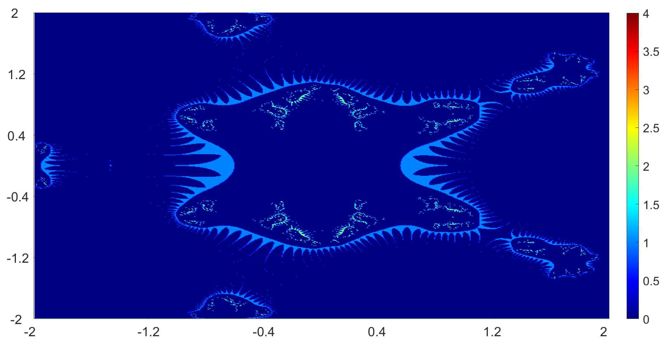
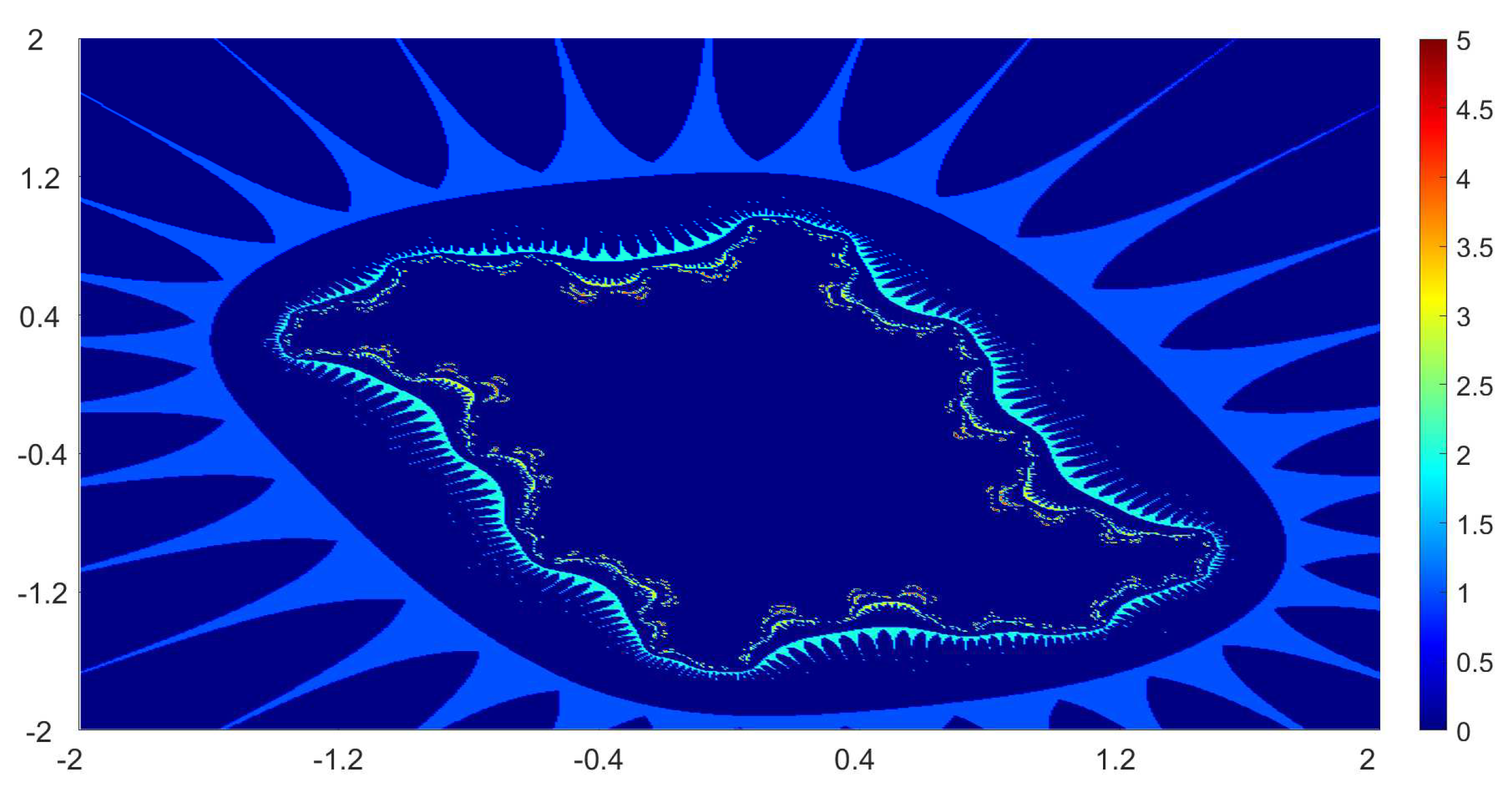
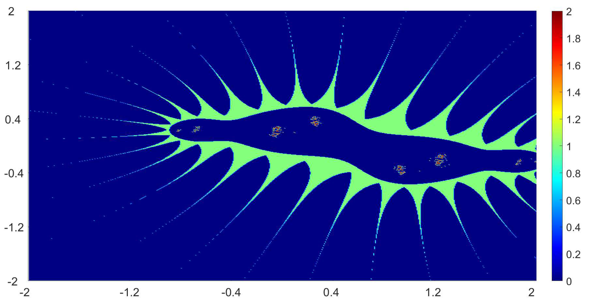
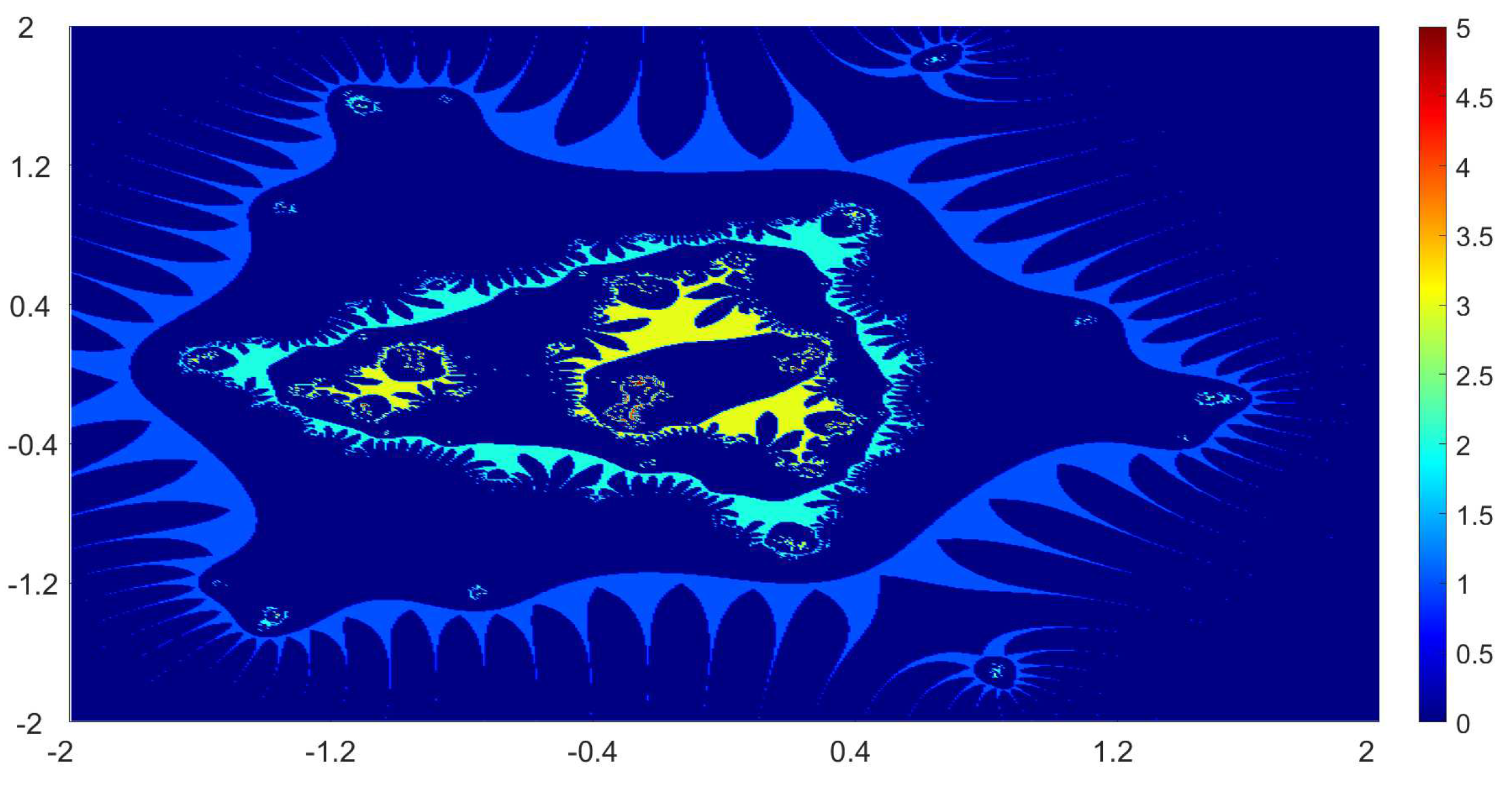
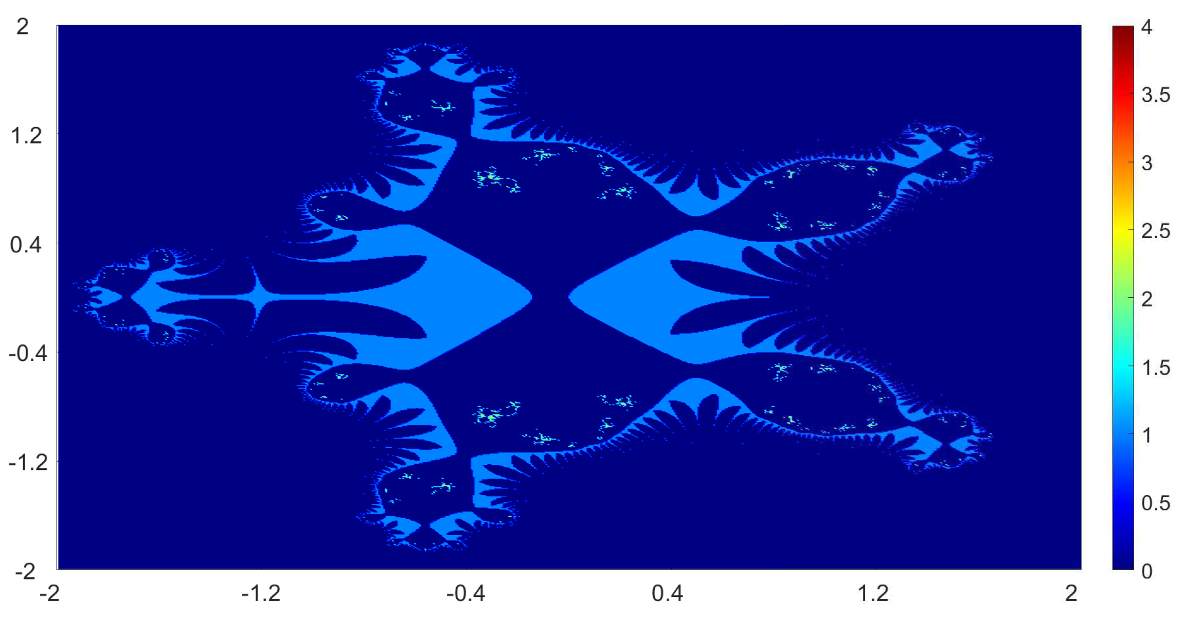
Now, we present the biomorphs generated by using Algorithm 1. For all our examples, we choose $A=[x_{min},x_{max}]\times [y_{min},y_{max}]=[-2,2]\times [-2,2],$ $s=600,$ $\epsilon =10,$ $K=5.$

Example 1.

We consider the polynomial$Q\left(x\right)=x^2+(-0.5+0.7\mathbf{i})x+(-0.1+0.18\mathbf{i}).$We vary the values of r and parameters$\alpha ,\mu ,\eta$as follows:

(a) 

$r=0.64,$$\mu =0.31,\eta =0.631,\alpha =0.513;$

(b) 

$r=0.32$$\mu =0.15,\eta =0.289,\alpha =0.720;$

(c) 

$r=2.5\mathbf{i},$$\mu =0.05,\eta =0.731,\alpha =0.910;$

(d) 

$r=-5\mathbf{i},$$\mu =0.790,\eta =0.487,\alpha =0.834.$

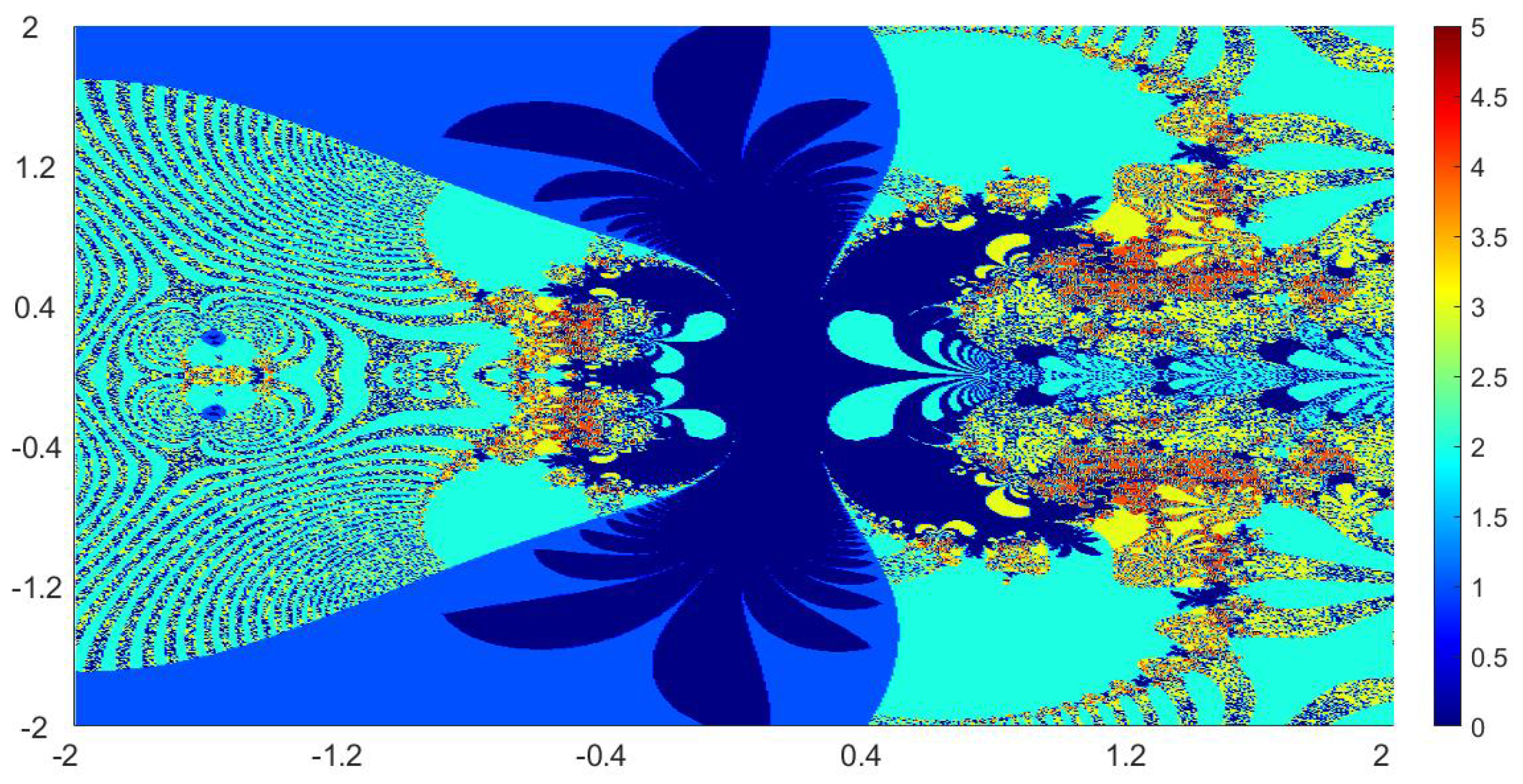
Figure 1, Figure 2, Figure 3 and Figure 4 present the obtained biomorphs. From the images, we see that the change in the parameters alters the colours and shapes of the biomorphs. Moreover, we can observed that the use of complex value of r adds swirls and twists to the obtained patterns. This makes the images look more dynamics and vivid.

Example 2.

In this example, we consider the quadratic polynomial$Q\left(x\right)=2x^2-3x$and choose the parameter$r=r_n$using the following switching technique [29], i.e.,

$$\left\{\begin{array}{c}{r}_0=t_1,\hfill \\ r_{2n-1}=\frac{1}{t_1^{2n-1}}-r_{2n-2},n\ge 1,\hfill \\ r_{2n}=\frac{1}{t_2^{2n}}-r_{2n-1},n\ge 1,\hfill \end{array}\right.$$

(11)

where$t_1,t_2$are non-zero complex variables. We fixed the parameters$\mu =0.591,\eta =0.327,\alpha =0.614$and vary the values of$t_1$and$t_2$as follows:

(a) 

$t_1=0.88,t_2=1.25;$

(b) 

$t_1=1.87,t_2=3.19;$

(c) 

$t_1=2+0.89\mathbf{i}$, $t_2=-2+0.77\mathbf{i};$

(d) 

$t_1=0.89\mathbf{i},$$t_2=0.61\mathbf{i}.$

The generated biomorphs are shown in Figure 5, Figure 6, Figure 7 and Figure 8. In the switching technique, it is seen that a small change in the values of $t_1$ and $t_2$ caused significant changes in the shapes, colours and dynamics of the biomorphs.

Example 3.

We consider the cubic polynomial$Q\left(x\right)=x^3+x^2-3x+1$and choose$r_n$using the switch technique as in the previous example. We vary the values of$t_1,t_2,\mu ,\eta$and α as follows:

(a) 

$t_1=0.89\mathbf{i},t_2=0.68\mathbf{i},\mu =0.5,\eta =0.09,\alpha =0.25;$

(b) 

$t_1=0.39,t_2=3.5,\mu =0.15,\eta =0.49,\alpha =0.325;$

(c) 

$t_1=-0.39,t_2=-2,\mu =0.35,\eta =0.15,\alpha =0.625;$

(d) 

$t_1=1.68\mathbf{i},t_2=-2.89,\mu =0.75,\eta =0.69,\alpha =0.425.$

Figure 9, Figure 10, Figure 11 and Figure 12 show the generated biomorphs. It is seen that a small change in the value of the parameters caused significant change in the shapes and dynamics of the biomorphs.

Example 4.

We consider the polynomial$Q\left(x\right)=x^6+x^2+1$and vary the values of$r,\mu ,\eta ,\alpha$as follows:

(a) 

$r=0.68,\mu =0.275,\eta =0.169,\alpha =0.343;$

(b) 

$r=0.37,\mu =0.0569,\eta =0.0175,\alpha =0.0521;$

(c) 

$r=0.037,\mu =0.175,\eta =0.0331,\alpha =0.0221;$

(d) 

$r=0.0037,\mu =0.0175,\eta =0.00331,\alpha =0.00221.$

The obtained biomorphs are shown in Figure 13, Figure 14, Figure 15 and Figure 16. We see that the change in the parameters has great impact on the shape of the obtained biomorphs.

Example 5.

Finally, in this last example, we consider a complex hyper-function$Q\left(x\right)=x^x$with different values of r as follows:

(a) 

$r=0.15;$

(b) 

$r=0.35;$

(c) 

$r=0.45;$

(d) 

$r=0.55.$

We also take $\alpha =0.25,\mu =0.64,\eta =0.73.$ The obtained graphics are shown in Figure 17, Figure 18, Figure 19 and Figure 20. We note that the obtained biomorphs do not really have organismic structure, however, the obtained graphics are very fascinating from an artistic point of view. These can be of interest to someone working in automatic creation of nice looking objects and general artworks. Moreover, the change in the value of r produced different graphics with distinct colours, shapes and dynamics.

5. Conclusions

In this paper, a new general iteration was used to study the behaviour of biomorphs with complex polynomials. The escape criterion for quadratic, cubic and higher degree polynomials for the general iteration were presented. Some new sets of biomorphs were also generated. It was observed that the variation of parameters caused changes in the dynamics, colours and shapes of biomorphs in most cases. The obtained biomorphs are interestingly different in comparison to those obtained by Pickover (using standard Picard iteration) [25] and Gdawiec (using Mann and Ishikawa iterations) [29].

In our future research, we would like to extend the works of Negi et al. [34] and Rani et al. [35] on the noise in superior Mandelbrot set and superior Julia sets respectively to modified biomorphs introduced in this paper. Moreover, it is interesting to develop automatic biomorphs searching methods like those proposed in Ashlook et al. for Julia set [43,44]. Furthermore, we will like to study other category of fractals types of complex fractals and inversion fractals with respect to the generation of biomorphs.

Finally, we note that the work in this paper can be developed by using other non-standard iterations (see [37,45]) known in fixed point theory for generating biomorphs.

Publisher’s Note: MDPI stays neutral with regard to jurisdictional claims in published maps and institutional affliations.

References

1. Grigson, G. The Arts Today; Bodley Head: London, UK, 1935; pp. 71–109. [Google Scholar]
2. Britannica. Available online: https://www.britannica.com/art/biomorphic-art (accessed on 26 November 2020).
3. Rafati, V.; Sahba, F. “Bahai temples”. In Encyclopædia Iranica; Springer: New York, NY, USA, 1989. [Google Scholar]
4. Zerbst, R. Antoni Gaudi–A Life Devoted to Architecture. Trans. from German by Doris Jones and Jeremy Gaines; Taschen: Hamburg, Germany, 1988; p. 30. ISBN 3-8228-0074-0. [Google Scholar]
5. Eidelberg, M.; Carmel, K. Design 1935–1965: What modern was: Selections from the Liliane and David M. In Stewart Collection, Montreal: Musée des arts Décoratifs de Montréal; Abrams: New York, NY, USA, 1991; p. 90. [Google Scholar]
6. Pina, L. Classic Herman Miller; Schiffer Publishing: Atglen, PA, USA, 1998; ISBN 0-7643-0471-2. [Google Scholar]
7. Negi, A.; Rani, M.; Mahanti, P.K. Computer simulation of the behavior of Julia sets using switching processes. Chaos Solitons Fractals 2008, 37, 1187–1192. [Google Scholar] [CrossRef]
8. Andreadis, I.; Karakasidis, T.E. On a topological closeness of perturbed Julia sets. Appl. Math. Comput. 2010, 217, 2883–2890. [Google Scholar] [CrossRef]
9. Peitgen, H.O.; Jurgens, H.; Saupe, D. Chaos and Fractals; Springer: New York, NY, USA, 1992. [Google Scholar]
10. Rani, M.; Negi, A. New Julia sets for complex Carotid–Kundalini function. Chaos Solitons Fractals 2008, 36, 226–236. [Google Scholar] [CrossRef]
11. Lei, T. Similarity between the Mandelbrot sets and Julia sets. Commun. Math. Phys. 1990, 134, 587–617. [Google Scholar] [CrossRef]
12. Mandelbrot, B.B. The Fractal Geometry of Nature; W. H. Freeman: San Francisco, CA, USA, 1982. [Google Scholar]
13. Crilly, A.J.; Earnshaw, R.A.; Jones, H. Fractals and Chaos; Springer: New York, NY, USA, 1991. [Google Scholar]
14. Devaney, R.L. A First Course in Chaotic Dynamical Systems: Theory and Experiment; Addison-Wesley: Boston, MA, USA, 1992. [Google Scholar]
15. Branner, B.; Hubbard, J.H. The iteration of cubic polynomials Part I: The global topology of parameter space. Acta Math. 1988, 160, 143–206. [Google Scholar] [CrossRef]
16. Branner, B.; Hubbard, J.H. The iteration of cubic polynomials Part II: Patterns and parapatterns. Acta Math. 1992, 169, 229–325. [Google Scholar] [CrossRef]
17. Frame, M.; Robertson, J. A generalized Mandelbrot set and the role of critical points. Comput. Graph. 1992, 16, 35–40. [Google Scholar] [CrossRef]
18. Geum, Y.H.; Hare, K.G. Groebner basis, resultants and the generalized Mandelbrot set. Chaos Solitons Fractals 2009, 42, 1016–1023. [Google Scholar] [CrossRef]
19. Rani, M.; Kumar, V. Superior Julia set. Res. Math. Educ. 2004, 8, 261–277. [Google Scholar]
20. Rani, M.; Kumar, V. Superior Mandelbrot set. Res Math Educ. 2004, 8, 279–291. [Google Scholar]
21. Chauhan, Y.S.; Rana, R.; Negi, A. New Julia sets of Ishikawa iterates. Int. J. Comput. Appl. 2010, 7, 34–42. [Google Scholar] [CrossRef]
22. Chauhan, Y.S.; Rana, R.; Negi, A. Complex dynamics of Ishikawa iterates for non integer values. Int. J. Comput. Appl. 2010, 9, 9–16. [Google Scholar] [CrossRef]
23. Rani, A.; Chugh, R. Julia sets and Mandelbrot sets in Noor orbit. Appl. Math. Comput. 2014, 228, 615–631. [Google Scholar]
24. Abbas, M.; Iqbal, H.; Sen, M.D.L. Generation of Julia and Madelbrot sets via fixed points. Symmetry 2020, 12, 86. [Google Scholar] [CrossRef] [Green Version]
25. Pickover, C.A. Biomorphs: Computer Displays of Biological Forms Generated from Mathematical Feedback Loops. Comput. Graph. Forum 1986, 5, 313–316. [Google Scholar] [CrossRef]
26. Levin, M. Morphogenetic Fields in Embryogenesis, Regeneration, and Cancer: Non-local Control of Complex Patterning. BioSystems 2012, 109, 243–261. [Google Scholar] [CrossRef] [Green Version]
27. Leys, J. Biomorphic Art: An Artist’s Statement. Comput. Graph. 2002, 26, 977–979. [Google Scholar] [CrossRef]
28. Mojica, N.S.; Navarro, J.; Marijuán, P.C.; Lahoz-Beltra, R. Cellular “bauplants”: Evolving Unicellular Forms by Means of Julia Sets and Pickover Biomorphs. BioSystems 2009, 98, 19–30. [Google Scholar] [CrossRef]
29. Gdawiec, K.; Kotarski, W.; Lisowska, A. Biomorphs via modified iterations. J. Nonlinear Sci. Appl. 2016, 9, 2305–2315. [Google Scholar] [CrossRef]
30. Mann, W.R. Mean Value Methods in Iteration. Proc. Amer. Math. Soc. 1953, 4, 506–510. [Google Scholar] [CrossRef]
31. Ishikawa, S. Fixed Points by a New Iteration Method. Proc. Amer. Math. Soc. 1974, 44, 147–150. [Google Scholar] [CrossRef]
32. Noor, M.A. New approximation schemes for general variational inequalities. J. Math. Anal. Appl. 2000, 251, 217–229. [Google Scholar] [CrossRef] [Green Version]
33. Agarwal, R.; Agarwal, V. Dynamic noise perturbed generalized superior Mandelbrot sets. Nonlinear Dyn. 2011, 67, 1883–1891. [Google Scholar] [CrossRef]
34. Negi, A.; Rani, M. A new approach to dynamic noise on superior Mandelbrot set. Chaos Solitons Fractals 2008, 36, 1089–1096. [Google Scholar] [CrossRef]
35. Rani, M.; Agarwal, R. Effect of stochastic noise on superior Julia sets. J. Math. Imaging Vis. 2010, 36, 63–68. [Google Scholar] [CrossRef]
36. Singh, S.L.; Jain, S.; Mishra, S.N. A New Approach to Superfractals. Chaos Solitons Fractals 2009, 42, 3110–3120. [Google Scholar] [CrossRef]
37. Gdawiec, K.; Kotarski, W.; Lisowski, A. Polynomiography based on the nonstandard Newton-like root finding methods. Abstr. Appl. Anal. 2015, 2015, 19. [Google Scholar] [CrossRef] [Green Version]
38. Gdawiec, K.; Shahid, A.A.; Nazeer, W. Higher order methods of the Basic Family of Iterations via S-iteration with s-convexity. Mediterr. J. Math. 2020, 17, 43. [Google Scholar] [CrossRef] [Green Version]
39. Kotarski, W.; Gdawiec, K.; Lisowska, A. Polynomiography via Ishikawa and Mann iterations. Lect. Notes Comput. Sci. 2012, 7431, 305–313. [Google Scholar] [CrossRef]
40. Garodia, C.; Uddin, I.; Khan, S.H. Approximating common fixed point by a new faster iteration. accepted.
41. Nazeer, W.; Kang, S.M.; Tanveer, M.; Shahid, A.A. Fixed point results in the generation of Julia and Mandelbrot sets. J. Ineq. Appl. 2015, 2015, 298. [Google Scholar] [CrossRef] [Green Version]
42. Proakis, J.G.; Manolakis, D.G. Digital Signal Processing: Principles, Algorithms and Applications, 4th ed.; Pearson: Bengaluru, India, 2007. [Google Scholar]
43. Ashlock, D.; Brown, J.A. Fitness Functions for Searching the Mandelbrot Set. In Proceedings of the 2011 IEEE Congress on Evolutionary Computation, New Orleans, LA, USA, 5–8 June 2011; pp. 1108–1115. [Google Scholar]
44. Ashlock, D.; Jamieson, B. Evolutionary Exploration of Generalized Julia Sets. In Proceedings of the IEEE Symposium on Computational Intelligence in Image and Signal Processing, Honolulu, HI, USA, 1–5 April 2007; pp. 163–170. [Google Scholar]
45. Gdawiec, K.; Kotarski, W. Polynomiography for the polynomial infinity norm via Kalantari’s formula and nonstandard iterations. Appl. Math. Comput. 2017, 307, 17–30. [Google Scholar] [CrossRef] [Green Version]
Figure 1. Example 1(a).
Mathematics 08 02172 g001
Figure 2. Example 1(b).
Mathematics 08 02172 g002
Figure 3. Example 1(c).
Mathematics 08 02172 g003
Figure 4. Example 1(d).
Mathematics 08 02172 g004
Figure 5. Example 2(a).
Mathematics 08 02172 g005
Figure 6. Example 2(b).
Mathematics 08 02172 g006
Figure 7. Example 2(c).
Mathematics 08 02172 g007
Figure 8. Example 2(d).
Mathematics 08 02172 g008
Figure 9. Example 3(a).
Mathematics 08 02172 g009
Figure 10. Example 3(b).
Mathematics 08 02172 g010
Figure 11. Example 3(c).
Mathematics 08 02172 g011
Figure 12. Example 3(d).
Mathematics 08 02172 g012
Figure 13. Example 4(a).
Mathematics 08 02172 g013
Figure 14. Example 4(b).
Mathematics 08 02172 g014
Figure 15. Example 4(c).
Mathematics 08 02172 g015
Figure 16. Example 4(d).
Mathematics 08 02172 g016
Figure 17. Example 5(a).
Mathematics 08 02172 g017
Figure 18. Example 5(b).
Mathematics 08 02172 g018
Figure 19. Example 5(c).
Mathematics 08 02172 g019
Figure 20. Example 5(d).
Mathematics 08 02172 g020