Estimation of Synaptic Activity during Neuronal Oscillations

Abstract

In the study of brain connectivity, an accessible and convenient way to unveil local functional structures is to infer the time trace of synaptic conductances received by a neuron by using exclusively information about its membrane potential (or voltage). Mathematically speaking, it constitutes a challenging inverse problem: it consists in inferring time-dependent parameters (synaptic conductances) departing from the solutions of a dynamical system that models the neuron’s membrane voltage. Several solutions have been proposed to perform these estimations when the neuron fluctuates mildly within the subthreshold regime, but very few methods exist for the spiking regime as large amplitude oscillations (revealing the activation of complex nonlinear dynamics) hinder the adaptability of subthreshold-based computational strategies (mostly linear). In a previous work, we presented a mathematical proof-of-concept that exploits the analytical knowledge of the period function of the model. Inspired by the relevance of the period function, in this paper we generalize it by providing a computational strategy that can potentially adapt to a variety of models as well as to experimental data. We base our proposal on the frequency versus synaptic conductance curve ($f-g_{syn}$), derived from an analytical study of a base model, to infer the actual synaptic conductance from the interspike intervals of the recorded voltage trace. Our results show that, when the conductances do not change abruptly on a time-scale smaller than the mean interspike interval, the time course of the synaptic conductances is well estimated. When no base model can be cast to the data, our strategy can be applied provided that a suitable $f-g_{syn}$ table can be experimentally constructed. Altogether, this work opens new avenues to unveil local brain connectivity in spiking (nonlinear) regimes.

1. Introduction

Estimating non-measurable connectivity parameters from experimental measurements is an important challenge to understand brain function. Brain activity is mainly driven by the intrinsic dynamics of neurons and their mutual connections, which are essentially regulated by synapses. A thorough knowledge of individual membrane potentials and synaptic terms is, therefore, crucial to understand how the brain operates. However, we are far from this utopia: current recording methods can only retrieve partial information, such as the time evolution of membrane potential of one or a few neurons. Unfortunately, other quantities that shape the connectivity, like synaptic conductances, are impossible to be directly recorded in experiments.

The time course of synaptic conductances arriving at a single cell not only provides local information about its functional connectivity, but it often constitutes an indicator to validate more general theories such as obtaining information about the architecture of the cortex, discerning between phase insensitive or spatial phase selective coupling [1], unveiling whether the integrative properties of cortical neurons are altered under high-conductance states [2], as well as studying many neuronal problems related to the balance between excitation and inhibition [3]. Unfortunately, there are no direct methods to estimate synaptic conductances, and thus they have to be deduced from experimentally observable quantities. As no direct methods are known to estimate synaptic conductances, they have to be deduced from experimentally observable quantities. This leads to the need of using inverse mathematical methods. As for many inverse problems, it has been proved to be an arduous analytical and computational task for which no general procedures are yet available.

Different strategies have been developed to estimate the time course of the synaptic conductances from time series of the membrane potential. Most strategies are based on deterministic linear estimation procedures (see [3,4,5,6,7]). However, researchers are aware of possible misestimations coming from the measurement noise produced during recordings. Therefore, new methods have been also devised to solve this problem from different approaches: stochastic linear procedures (see [8,9,10,11,12,13]), sophisticated filtering techniques (see [14,15,16,17,18]), and techniques using the $I-V$ relation extracted experimentally (see [19]).

Even though all these strategies provide circumstantial solutions, it is also well known that they can only be applied in the subthreshold regime, where ionic currents are negligible (see [20,21]), a situation for which simplified models (close to linear) are representative enough to account for the voltage dynamics. However, it has also been demonstrated that these linear procedures can also provide wrong estimations when ionic currents are active in the subthreshold regime causing non-spikes in the membrane potential of the postsynaptic neuron. This fact motivates the introduction of new strategies to estimate conductances under these nonlinear paradigms (see [22,23]). More recently, in [24], the authors identify that another artifact that can provide wrong estimations is to assume that the synaptic conductances are voltage-independent; to avoid this problem, they provide a new estimation procedure, also in the linear framework. Despite the many efforts in the literature to get rid of artifacts that can contaminate the estimation of conductances (influence of noise, activity of subthreshold ionic currents, variability across trials, etc.), one of the most resilient troubles are the nonlinearities that the $f-I$ curve exhibits in the presence of spiking mechanisms.

On the other hand, a line of research is devoted to look for possible strategies to estimate conductances in the spiking regime. For instance, in [25], the authors use a firing clamp technique where a description of the spike is given in terms of the membrane potential threshold and the amplitude of the spike. These traces are approximated by calibrating the membrane potential using dynamic clamp in in vitro experiments of isolated neurons and a quadratic polynomial approximation. More recently, in [26] we introduce a mathematical approach to estimate conductances by characterizing the period of the membrane potential, and in [27] estimations of the conductances of spike trains of the membrane potential are performed.

In [26], we present a first proof-of-concept to estimate synaptic conductances in the spiking regime based on information about the $f-I$ curve of the neuron. The idea was exemplified with the McKean model, a piecewise linear system that allows for a quasi-analytic expression of the $f-I$ curve. More specifically, we approximated the firing period, T, as a function of the parameters of the system and, in particular, of the synaptic conductance parameter, $g_{syn}$. Therefore, for a given interspike interval (ISI) of length $T^{*}$, one can numerically solve the implicit equation $T\left(g_{syn}\right)=T^{*}$ to obtain an estimation, $g_{syn,est}$, of the synaptic conductances during that ISI. In order to obtain the time course of the synaptic conductances, the procedure is repeated for each ISI. By interpolation, a continuous estimation of $g_{syn,est}\left(t\right)$ can be obtained, which is proved to be an accurate estimation of the prescribed conductances provided that they have slower variation (in time) than the membrane potential. Although the results obtained in [26] show that using the $f-I$ to estimate synaptic conductances in spiking regimes can be a suitable strategy, there were only applied to the McKean model, a very specific and non-realistic model, which is nothing but a caricature of the Fitzhugh–Nagumo system.

An improvement of this estimation procedure is to consider a different underlying mathematical model that could better fit experimental data. On the one hand, desirable candidates would be conductance-based models as per the Hodgkin–Huxley formalism but, even though some of them (pyramidal cells [28], stellate cells [29], etc.) have been investigated in the context of estimation of conductances in subthreshold regimes, it is extremely difficult to devise a procedure for a generic conductance-based model. On the other hand, integrate-and-fire (IF) models have also been considered as good approximations to the neuronal activity of different type of neurons (see [30,31,32,33,34]) and are simple enough. We found that the exponential integrate-and-fire (EIF) model represents an optimal balance between adaptability to experimental data and computational $f-I$ curves, and model simplicity.

In this paper, following the ideas introduced in [26], we propose a procedure to estimate conductances under a regular spiking regime. This procedure is based on a modification of the standard frequency–input curve, which consists of replacing the input constant current by a constant synaptic conductance ($f-g_{syn}$ curve). We aim to estimate the global synaptic conductance time course from a membrane potential time series of a spiking neuron, for which we can have an accurate $f-g_{syn}$ curve. For simplicity, here we assume that all synaptic input is excitatory.

The $f-g_{syn}$ curve can be provided in several ways: (I) from dynamic clamp experiments, using in vitro recording; (II) approximating the real data by a base model (IIa) for which we can obtain an analytic expression for the $f-g_{syn}$ curve, such as the leaky or the quadratic integrate-and-fire models (see [35,36]), or (IIb) allowing an approximate expression for the $f-g_{syn}$ curve, such as the McKean model (see [26]) or the exponential integrate-and-fire (see Section 2.1); finally, (III) using a more detailed model that can be numerically integrated in order to construct a $f-g_{syn}$ curve table, that is, providing a set of period-conductance pairs extracted from numerical experiments (see Section 2.2). Once the $f-g_{syn}$ relationship is obtained, we have an expression of the period $T=1/f$ depending on the conductances (or vice versa). In cases (I) and (III), where we have a discretization of this relationship, in order to obtain a continuous function $T\left(g_{syn}\right)$, one can interpolate the data using, for instance, the piecewise cubic Hermite interpolating polynomial (PCHIP). Therefore, given an interspike interval $T^{*}$, the corresponding conductance within this interval can be obtained by solving analytically or numerically the equation $T\left(g_{syn}\right)=T^{*}$.

Notice that for case (I), which involves dynamic clamp, the method can be considered to extract the $f-g_{syn}$ curve in in vitro experiments but not in in vivo as several injected currents would be required in order to have a precise $f-g_{syn}$ curve, which could add both variability across trials and noise measurement. Alternatively, we provide different computational strategies (II–III) to obtain the $f-g_{syn}$ curve. Even though strategies (IIa) and (IIb) provide good approximations to the $f-g_{syn}$ curve, they should not be applied in general to approximate the $f-g_{syn}$ curve for a wider range of neurons. For this reason, the computational approach presented in Section 2.2 focuses on the idea of case (III).

The paper is organized as follows. In Section 2.1, we present the neuronal model we use to generate data by means of prescribed conductances and its approximation to the EIF model. In Section 2.2, we present the estimation procedure giving a pseudocode of its implementation sketched in Figure 1. Next, in Section 3, we show the results of the estimation procedures. Finally, in Section 4 and Section 5 we discuss the results obtained and present our conclusions.

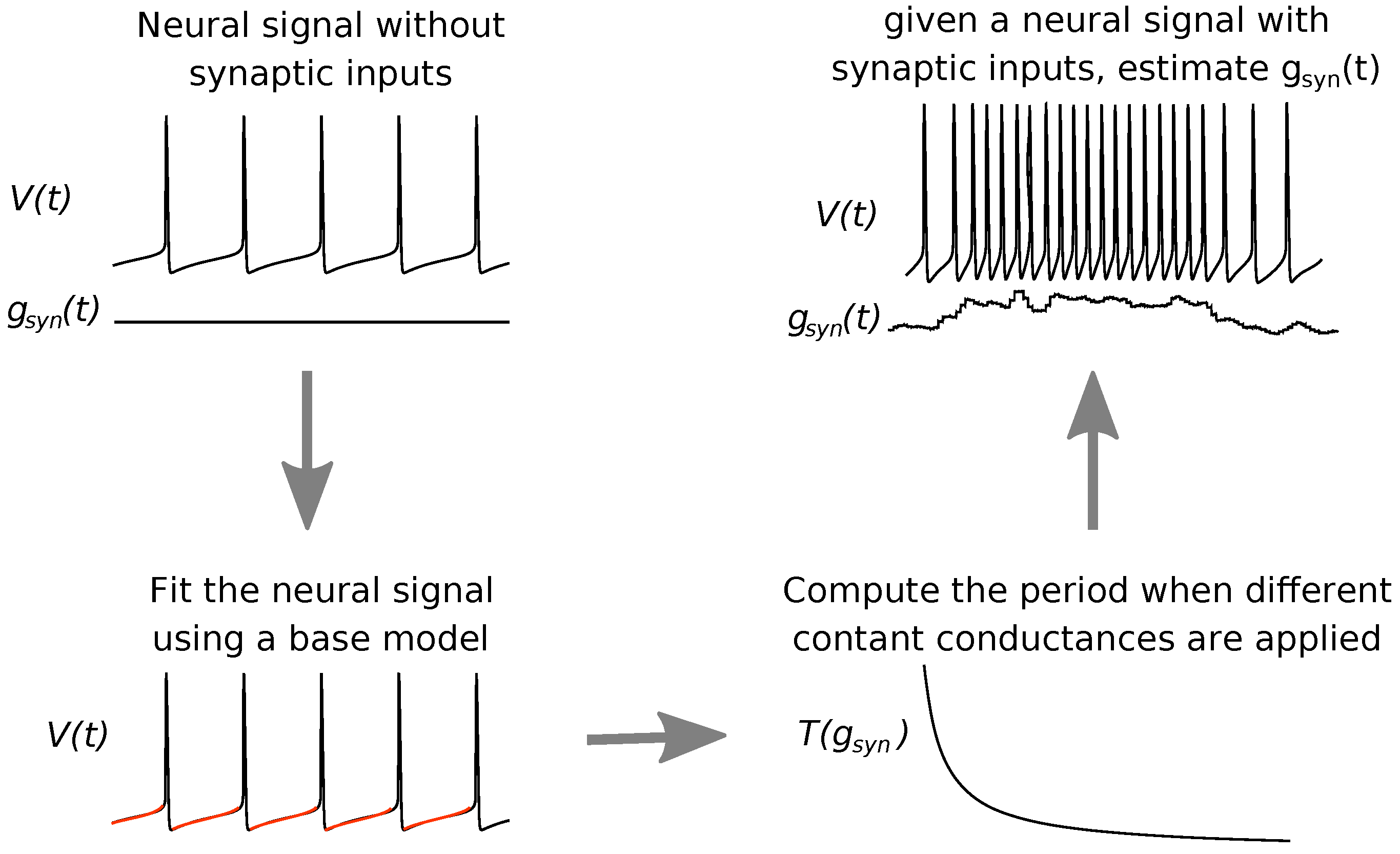
Figure 1. Scheme of the estimation procedure performed by Algorithm 1. Given a neural signal from a neuron which is not receiving synaptic inputs ($g_{syn}\left(t\right)=0$; upper left) but exhibiting regular spiking, we fit this signal using a computational model where the synaptic term is added afterwards (bottom left, where the red color stands for the fitting). Next, we use this model to compute the period (or frequency) for different constant synaptic conductances ($T\left(g_{syn}\right)$, bottom right). We finally estimate the synaptic conductance time course from a neural signal subjected to synaptic inputs (upper right).

Figure 1. Scheme of the estimation procedure performed by Algorithm 1. Given a neural signal from a neuron which is not receiving synaptic inputs ($g_{syn}\left(t\right)=0$; upper left) but exhibiting regular spiking, we fit this signal using a computational model where the synaptic term is added afterwards (bottom left, where the red color stands for the fitting). Next, we use this model to compute the period (or frequency) for different constant synaptic conductances ($T\left(g_{syn}\right)$, bottom right). We finally estimate the synaptic conductance time course from a neural signal subjected to synaptic inputs (upper right).

Algorithm 1 Estimation procedure

Data collection. Let ${\mathcal{V}}_0:=\{V\left(t\right),t\in J\}$ be the membrane potential of a neuron $\mathcal{N}$ on some time interval J in absence of synaptic inputs. Fitting data to a base model. Fit ${\mathcal{V}}_0$ to a base model (for instance, an integrate-and-fire model). Call $\mathcal{P}$ the set of parameters of the base model that gives the best fitting. The $f-g_{syn}$ curve for the base model. Build up the function $G_{syn}\left(T\right)$ for the base model with the set $\mathcal{P}$. Depending on the base model, one possibility is to find either $G_{syn}$ analytically, or its inverse $T\left(g_{syn}\right)$ and then invert it. Otherwise, we will proceed computationally: (a) Consider a discretization of N equally-spaced synaptic conductances, that is, ${\left\{g_{syn,i}\right\}}_{i=1}^N$ where $g_{syn,i+1}-g_{syn,i}={\delta }_g$, for all $i=1\dots N-1$, where ${\delta }_g>0$ is a constant, assuming that the base model is regularly spiking for $g_{syn}\in [g_{syn,0},g_{syn,N}]$. (b) By numerical integration, for each $g_{syn,i}$ with $i=1\dots N$, obtain the period ${\widehat{T}}_i$ of the corresponding membrane potential. Note that this correspondence could also be obtained using one of the three other options presented in the Introduction (page 3). In all cases, a table containing the relation between $\widehat{T}$ and $g_{syn}$ is obtained. Then, interpolate it to obtain a continuous function $G_{syn}\left(T\right)$ using, for instance, a piecewise cubic Hermite interpolating polynomial (PCHIP). Estimation: computing ISIs. Let $\mathcal{V}=\{V\left(t\right),t\in J^{\prime }\}$ be the membrane potential trace, for some time interval $J^{\prime }$, of neuron $\mathcal{N}$ subject to synaptic input bombardments. Assume that $\mathcal{N}$ emits $n_{spk}$ spikes along the time span $J^{\prime }$ and let $T_j$, for $j=1,\cdots ,n_{spk}$, be the j-$th$ interspike interval of $\mathcal{V}$. Estimation: inference. For each $T_j$, $j=1\dots n_{spk}$, compute $G_{syn}\left(T_j\right)$ to obtain the corresponding estimated conductance ${\widehat{g}}_{syn,j}$. Estimation: interpolation. Interpolate the set ${\left\{(t_j,{\widehat{g}}_{syn,j})\right\}}_{j=1}^{n_{spk}}$, where $t_j$ is a point on the $j-th$ ISI. Here, we take $t_j$ the endpoint of the $j-th$ ISI and use a piecewise cubic Hermite interpolating polynomial (PCHIP). * Note that for those models such that a qualitative expression of the $T-g_{syn}$ curve can be provided, the interpolation step does not proceed.

2. Methods

In this section, we present the estimation procedure we use to estimate conductances from a neuronal signal that contains high activity (Section 2.2). In order to prove the efficiency of the procedure, we need to generate in silico data by specifying the actual conductances. These data are the input of the procedure, whose output is compared with the actual conductances. Then, we also present here the neural models we use and the prescribed synaptic drive (Section 2.1).

2.1. Models and Data Treatment

2.1.1. Neuronal Models

Along the paper, we consider different neuronal models both for the purpose of generating membrane potential traces and to use them as base models for the estimations of synaptic conductances. We keep the choice of models minimal; as we mention in other parts of the paper, we can adapt our procedure to many other models.

Pyramidal cell model

We first consider a simplified version of a model for a pyramidal neuron (see [28]), where only the soma compartment has been considered. It is a spiking model driven by the interaction of sodium $\left(I_{Na}\right)$ and potassium $\left(I_K\right)$ currents. The membrane potential V follows the differential equation

$$C_m\frac{dV}{dt}=-I_L-I_{Na}-I_K+I_{app}-I_{syn},$$

(1)

where $C_m$ is the capacitance, $I_{syn}$ is the synaptic current, $I_{app}$ is the applied current, $I_L$ is the leak current, and $I_{Na}$ and $I_K$ are the ionic currents, which are described by equations

$$\begin{array}{c}{I}_L=g_L(V-V_L),\hfill \\ I_{Na}=g_{Na}{m}_{\infty }^3\left(V\right)h(V-V_{Na}),\hfill \\ I_K=g_K{n}^4(V-V_K),\hfill \end{array}$$

where $V_x$ and $g_x$, with $x\in \{L,Na,K\}$, represent the specific reversal potentials and maximal conductances, respectively. The variables h and n are gating variables governed by first-order kinetics of type

$$\dot{w}=\frac{dw}{dt}=\varphi [{\alpha }_w\left(V\right)(1-w)-{\beta }_w\left(V\right)w]=\varphi \frac{w_{\infty }\left(V\right)-w}{{\tau }_w\left(V\right)},$$

(2)

where w represents either h or n; $w_{\infty }\left(V\right):={\alpha }_w\left(V\right)/({\alpha }_w\left(V\right)+{\beta }_w\left(V\right))$ is the w steady state and ${\tau }_w\left(V\right)={({\alpha }_w\left(V\right)+{\beta }_w\left(V\right))}^{-1}$ is the w time decay. In our version of this model, the m-type (fast) variable is considered to be at the steady state $m=m_{\infty }\left(V\right)$.

The oscillatory regime for this model is approximately $I_{app}\in (0.225653,108.285)$$\mathsf{\mu }$A/cm${}^2$. By default, we take $I_{app}=0$ $\mathsf{\mu }$A/cm${}^2$ (see Appendix B in [20] for a justification of this choice).

For more details about the biophysical parameters of the model, see Appendix A.

We will also explore how the random synaptic input or measurement noise affects the estimation of conductances, and so we will add a noise term to the membrane potential Equation (1). For the sake of reference, we present the resulting system as a separate model.

Noisy pyramidal cell model

Considering a white noise process $\eta \left(t\right)$ having zero mean and standard deviation ${\sigma }_V$, system (1) writes as

$$C_m\frac{dV}{dt}=-I_L\left(t\right)-I_{Na}\left(t\right)-I_K\left(t\right)+I_{app}-I_{syn}\left(t\right)+\eta \left(t\right).$$

(3)

Stellate cell model

The stellate cell model is taken from [29]. The membrane potential dynamics is given by

$$C\frac{dV}{dt}=-I_L-I_{Na}-I_K-I_{NaP}-I_h+I_{app}-I_{syn},$$

(4)

where C is the membrane capacitance, $I_{syn}$ the synaptic current, and $I_{app}$ the applied current. The leakage and ion currents are given by

$$\begin{array}{c}{I}_L=g_L(V-V_L),\hfill \\ I_{Na}=g_{Na}{m}^3\left(V\right)h(V-V_{Na}),\hfill \\ I_K=g_K{n}^4(V-V_K),\hfill \\ I_{NaP}=g_{p}p(V-V_{Na}),\hfill \\ I_h=g_h(0.65r_f+0.35r_s)(V-V_h),\hfill \end{array}$$

where $V_x$ and $g_x$, for $x\in \{L,Na,K,NaP,h\}$, denote the corresponding ion reversal potentials and maximal conductances, respectively.

The gating variables w, which can be either m, h, n, p, $r_f$, or $r_s$, follow the same first-order dynamics (2) as for the pyramidal cell model.

In absence of synaptic inputs, this model presents spikes for an applied current greater that $I_T=-1.46\mathsf{\mu }$A/cm${}^2$. In our case, to have a high frequency of spikes, we inject a constant current equal to $I_{app}=8\mathsf{\mu }$A/cm${}^2$.

For more details about the biophysical parameters of the model, see Appendix A.

Exponential Integrate-and-Fire (EIF) model with constant adaptation

We chose the EIF model as representative of base models due to its well-known properties of being able to shape its parameters in order to fit to diverse $f-I$, see [30]. Therefore, it will be used during the estimation procedure of the synaptic conductances. We write it as

$$C_m\frac{dV}{dt}=g_L{∆}_{T}exp((V-V_T)/{∆}_T)-I_L-I_{syn}+I_{app}.$$

(5)

Here, $I_T$ is the largest input current for which the neuron does not spike, $V_T$ is the corresponding membrane potential on the $V-I$ curve, ${∆}_T$ stands for the spike slope factor (which is related to the sharpness of the spike initialization), and the rest of terms are described as in the pyramidal cell model (1).

When the membrane potential reaches the numerical threshold ${\vartheta }_{th}$, which defines the spiking time $t^{spike}$, the membrane potential is reset to $V_{reset}$ and the integration restarts at $t^{spike}+{∆}^{abs}$, where ${∆}^{abs}$ is the absolute refractory time (typically chosen between 0 and $5\mathrm{ms}$, see [37]).

To fit the pyramidal cell model (1), the specific EIF parameters have been set to be $I_T=0.16\mathsf{\mu }$A/cm${}^2$, $V_T=-59.9$ mV, ${∆}_T=2.97$ mV, ${\vartheta }_{th}=-51$ mV, $V_{reset}=-71$ mV, and ${∆}^{abs}=1.25$ ms (see Figure 2).

In this case, the interspike period can be computed as the time of flight between the reset value ($V_{reset}$) and the threshold (${\vartheta }_{th}$) for the voltage, adding the absolute refractory time (${∆}^{abs}$). By solving the differential Equation (5) in this range of membrane potential values, if $g_{syn}$ is considered constant, the interspike period is given by

$$T={\int }_{V_{reset}}^{{\vartheta }_{th}}{\displaystyle \frac{C_m}{g_L{∆}_{T}exp((V-V_T)/{∆}_T)-I_L-I_{syn}+I_{app}}}dV+{∆}^{abs}.$$

(6)

We note that this expression provides an implicit $T-g_{syn}$ relationship as $I_{syn}$ depends on $g_{syn}$. Therefore, for a specific conductance value, we can numerically solve it using a numerical method for integrals (see Section 2.1.3). Unfortunately, there is no method to further simplify this expression.

Note that Equation (6) can only be used if we suppose that $dV/dt$ is far from zero, that is, if we are not in the resting regime. However, for those specific time intervals where $dV/dt\approx 0$, from (5), the synaptic conductance is given by

$$g_{syn}\left(t\right)={\displaystyle \frac{g_L{∆}_{T}exp((V-V_T)/{∆}_T)-I_L+I_{app}}{V_{syn}}},$$

(7)

where $V=V\left(t\right)$.

2.1.2. Synaptic Drive

In our simulations we assume that the target neuron is stimulated through two different currents: (1) an external current, $I_{app}$, which is a constant value that places the cell in the excitable regime, ready to induce spiking activity within a biologically plausible frequency range, and (2) the synaptic input $I_{syn}$, which comes from other neurons of the network and eventually leads to the variation of the spike frequency.

In the different neural models, the synaptic input is always supposed to be of the form $I_{syn}=g_{syn}(V-V_{syn})$, where $g_{syn}=g_{syn}\left(t\right)$ is the synaptic conductance trace and $V_{syn}$ is the synaptic reversal potential; assumed to be excitatory in our simulations.

To generate the membrane potential of the neuron, we consider specific prescribed conductances. In our in silico experiments, we inject the corresponding synaptic currents, we extract the voltage response, and, pretending not to know them, we finally apply our methods to estimate the synaptic conductances. For this purpose, we use two different types of conductance traces: a synthetic three-frequency oscillatory drive and a more realistic trace obtained from a computational network. Note that, due to the nature of the problem we tackle here, there are no actual conductance traces available unless dynamic clamp experiments are performed.

We define the three-frequency oscillatory drive as

$$g_{syn}=A_{1}cos\left(\frac{2\pi }{T_1}t\right)+A_{2}cos\left(\frac{2\pi }{T_2}t\right)+A_{3}cos\left(\frac{2\pi }{T_3}t\right)+A_4,$$

(8)

being $A_1=0.0022$, $A_2=0.002$, $A_3=0.001$, $A_4=0.025$, $T_1=150$, $T_2=320$, and $T_3=50$. These values have been chosen to ensure a plausible spiking frequency for such kind of neurons. The resulting conductance trace is shown in Figure 3a (black curve); observe that it elicits a membrane potential completely immersed in the spiking regime (without silent periods interspersed), see Figure 3c.

On the other hand, to explore the synaptic regime interspersed by short silent periods, we chose a more realistic synaptic conductance input, consisting of a trace with a 1 ms resolution obtained from a computational network that models the layer 4C$\alpha$ of the primary visual cortex (see [1,38]). A small amount of noise has been added to these synaptic conductances of 0 mean and $0.0001$ deviation. The conductances trace is shown in Figure 4a (black curve).

2.1.3. Numerical Methods

As we are considering neural models described both by ODE and SDE systems, we need to use different numerical methods to integrate them.

To integrate the system of ordinary differential equations of the pyramidal cell model without noise, and also to integrate the EIF model used in the estimation procedure, we used the 4th-order Runge–Kutta method with a $0.01$ ms time step; the choice was made to sample our data with an accuracy similar to that obtained experimentally.

On the other hand, the noisy pyramidal cell model was integrated using the Euler–Maruyama method with a fixed time step of $0.01$ ms.

To compute a relation between interspikes intervals and constant synaptic conductances values (see Algorithm 1, step 3b), we consider a discretization of $g_{syn}$ separated ${\delta }_g=1\times {10}^{-3}\mathsf{\mu }$A/cm${}^2$ (unless otherwise stated).

For the interpolation of the estimated conductances, we use the Matlab function pchip, which is an implementation of the piecewise cubic Hermite interpolation. For our data sets, the errors induced by this method showed to be lower than those induced by the interpolation by cubic splines.

Finally, to numerically solve integrals, we use the Romberg method with positive integer $n=15$ to ensure an error of order ${10}^{-8}$ or lower (see [39]). When implicit equations need to be solved, we use the secant method with error tolerance ${10}^{-5}$.

2.2. Estimation Procedures

In order to estimate the synaptic conductances from the membrane potential trace we use similar ideas to those presented in [26]. In that paper, which was uniquely devoted to a piecewise linear system (the McKean model), the knowledge of an analytical approximation of the period T as a function of the synaptic conductance $g_{syn}$ was essential. However, as exposed in the Introduction, in general this analytical approximation cannot be obtained, and therefore we next propose a computational adaptation.

We first fit the in silico data, namely, the membrane potential, to a base model; here, we use the exponential (EIF) model, already described in Section 2.1.1.

Once we have determined the parameters of the base model, we integrate it for different constant synaptic conductances $g_{syn}$ and compute the period of oscillation, T. This results in a table of corresponding $T-g_{syn}$ pairs, which can further be interpolated, using for instance the PCHIP interpolation, to obtain a continuous function $G_{syn}\left(T\right)$.

Finally, given any membrane potential trace, we compute, for each interspike time interval (ISI), the ISI duration, $T^{*}$, and its corresponding $G_{syn}\left(T^{*}\right)$. Repeating the procedure for all the ISIs, we obtain a discrete trace of synaptic conductances, which can finally be interpolated using also the PCHIP interpolation.

A schematic representation of this estimation procedure is presented in Algorithm 1 and displayed in Figure 1.

Note that, in step 3b of Algorithm 1, several different synaptic conductances can provide the same period $\widehat{T}$. This lack of uniqueness is a trouble for the following steps in the algorithm. Even though in all cases we have treated, this issue had not happened, a control condition needs to be considered in this step to ensure the monotonic behavior in the $T-g_{syn}$ curve. Therefore, we have overcome this drawback by choosing the closest value to the last computed conductance.

3. Results

In order to test the estimation procedure, we apply Algorithm 1 (see Section 2.2) to membrane potential traces, often referred to as actual membrane potential traces, obtained computationally from the pyramidal cell model (see Section 2.1.1). This model will be considered either with additive noise (3), or without it (1). Moreover, in our simulations we consider the model with different synaptic drives to simulate spiking regimes without (Section 3.1) and with (Section 3.2) short subthreshold regimes interspersed (see Section 2.1.2 for more details in the synaptic drive).

For the different synaptic drives, we perform the estimation of conductances using different base models in Algorithm 1, step 3b. First, as we know that, by construction, the actual membrane potential follows the pyramidal neuron model, we consider this model as the base model, so we can test how powerful the estimation procedure is if we know the exact neural model. In this case, we deepen our results by exploring the cases where the data have been obtained with different amounts of noise and where the $T-g_{syn}$ curve has been constituted using different discretizations.

However, in most of the cases, the specific model that describes the neural data we have in consideration is not always known; therefore, an approximation of it is required. For this reason, second, we use the exponential integrate-and-fire (EIF) model with constant adaptation as a base model and try to approximate the activity of the pyramidal cells to it (as in [30]; see also Section 2.1).

Finally, we explore the situation of having a small sample of $(g_{syn},T\left(g_{syn}\right))$ pairs which are obtained with some additive noise rather than having a reference model to obtain a more precise $T-g_{syn}$ curve. This specific case could be given when trying to obtain the $T-g_{syn}$ curve experimentally, where data are obtained with measurement noise and variability across trials. In this case, we first generate a small sample of $(g_{syn},T\left(g_{syn}\right))$ pairs where we add a small bias in order to simulate possible errors in the recordings. Then, we use a proper fitting to obtain the $G_{syn}\left(T\right)$ curve to be able to proceed with the estimation procedure (see Section 3.1.4 for more details on how). We will refer to this curve as the $T-g_{syn}$ experimental curve.

In

Table 1. Outline of the different cases studied in Section 3 (Results).

Data Generation Model	Synaptic Drive	Base Model for the $\mathit{T}-{\mathit{g}}_{\mathit{syn}}$ Curve	Results	Figure	Errors
Pyramidal cell model (1)		Pyramidal cell model (1)	Section 3.1.1	Figure 3	Table 2
				Not shown	Table 3
	3-frequency oscillatory drive (8)	EIF model (5)	Section 3.1.3	Figure 5	Table 4
		EIF period function (6) and (7)	Section 3.1.3	Not shown
		Experiment-like curve	Section 3.1.4	Figures 6 and 7
Noisy pyramidal cell model (3)	From computational network (see [1,38])	Pyramidal cell model (1)	Section 3.2	Figure 8	Table 5
		EIF model (5)
		Experiment-like curve

, we provide a summary of the results found in the different subsections.

3.1. Estimation in the Spiking Regime

In this section, we present the results obtained from simulations of the noisy pyramidal cell model using the prescribed three-frequency oscillatory drive defined in (8). This configuration allows us to obtain a membrane potential trace in the spiking regime without interspersed silent periods. The estimation has been performed using, as base model, the three mentioned cases: the pyramidal cell model (Section 3.1.1), the EIF model (Section 3.1.3), and the $T-g_{syn}$ experimental curve (Section 3.1.4).

3.1.1. Estimation When the Neural Model Is Known

In this case, we apply the estimation procedure given in Algorithm 1 considering the pyramidal neural model as a base model in step 3b of the algorithm.

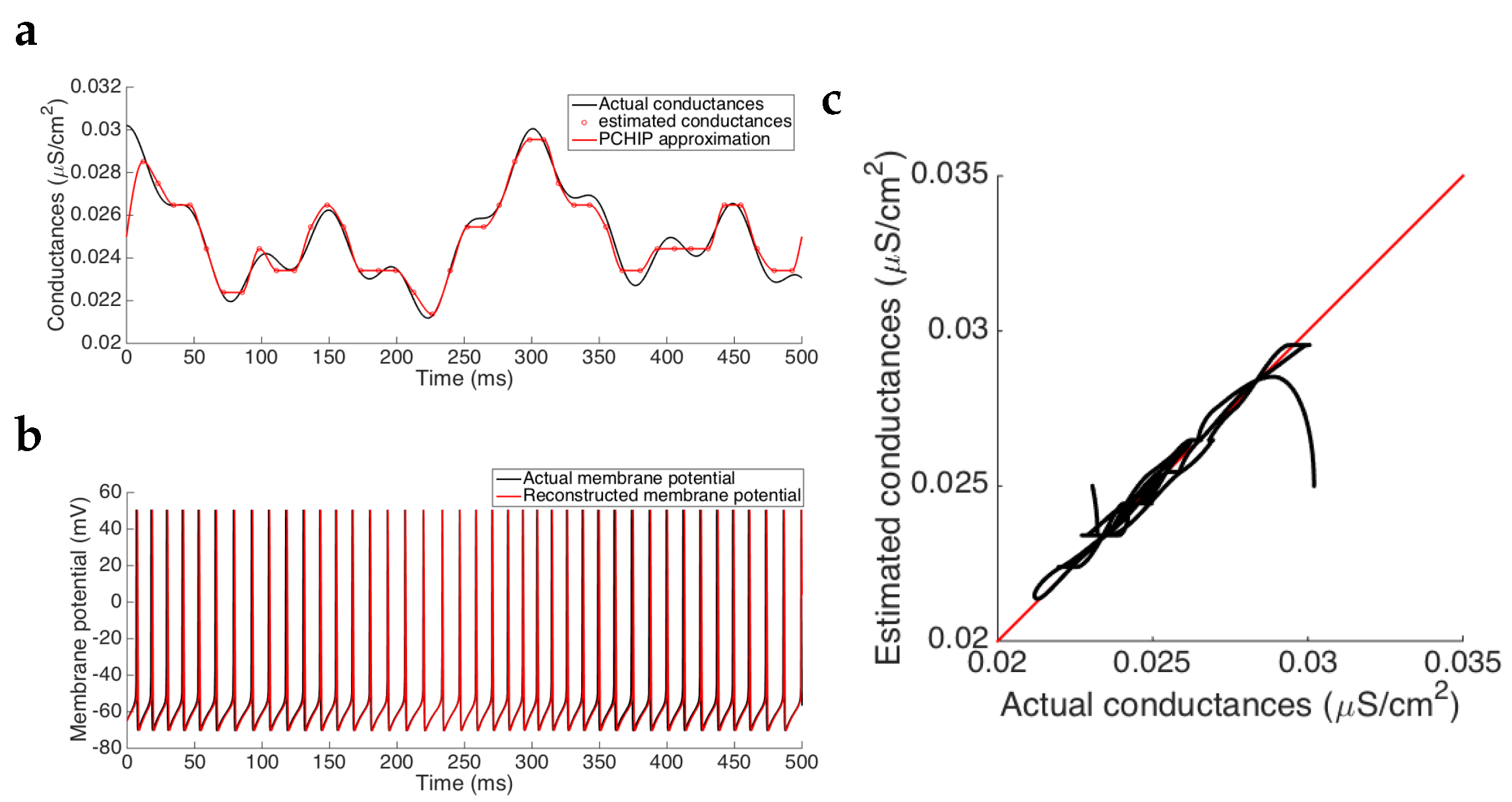
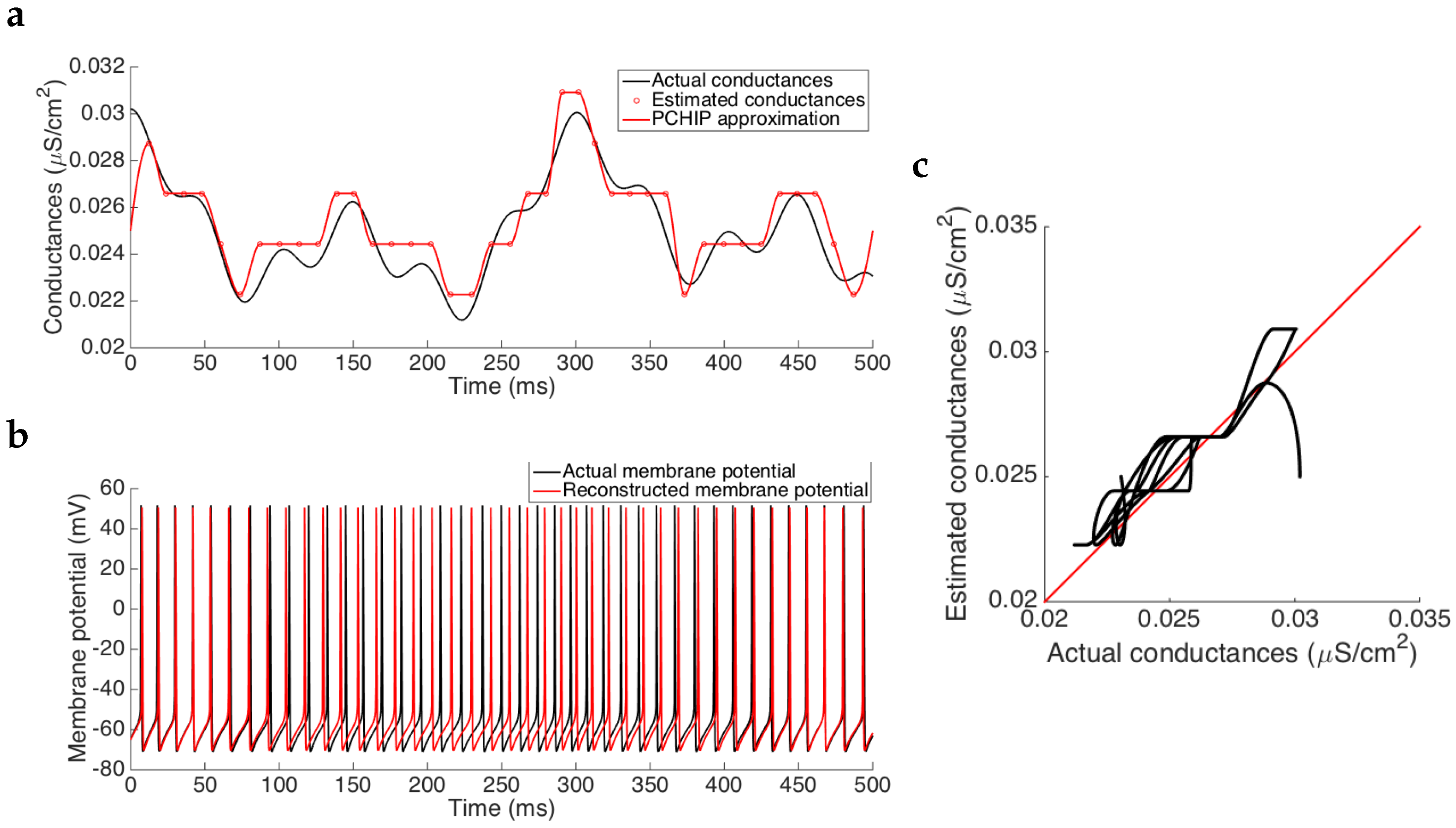
Results show that the estimated synaptic conductance trace follows the actual one before and after interpolating the estimated values (see Figure 3a). After a short transient discrepancy observed in the first 20 ms, due to the the fact that we cannot have an a priori guess of the actual initial conditions, we observe a strong agreement between the estimation and the actual values, as we can see in Figure 3c where the actual conductance trace versus the estimated one (after being interpolated) lies in the vicinity of the identity line, meaning a good approximation. In fact, computing the errors between the two traces, we have that the mean squared error is of order $O\left({10}^{-9}\right)$ and the relative error is, in mean, of order $O\left({10}^{-3}\right)$, indicating that the Algorithm 1 accurately estimates the synaptic conductance time course (see

Table 2. Errors caused by the discretization used for the period–conductance relationship. This table shows the errors caused in the estimation when the deterministic pyramidal cell model is used both to generate the actual membrane potential and as a base model in the estimation procedure. The first column shows the discretization of the conductances used to build up the table that relates the period with constant values of the conductance in Algorithm 1, step 3b. The second column shows the mean of the relative error of the estimation. Third column shows the mean squared error obtained in each case. The last column shows again the mean squared error obtained after interpolating the estimated conductances using the PCHIP interpolation.

${\mathit{g}}_{\mathit{syn}}$	Mean of	MSE	MSE
Discretization	the Relative Error	Estimated Values	Interpolated Values
${10}^{-5}$	$1.69\times {10}^{-3}$	$2.435\times {10}^{-9}$	$1.501\times {10}^{-7}$
${10}^{-4}$	$1.730\times {10}^{-3}$	$2.978\times {10}^{-9}$	$1.501\times {10}^{-7}$
${10}^{-3}$	$9.907\times {10}^{-3}$	$8.831\times {10}^{-8}$	$2.435\times {10}^{-7}$

). Note that, in this case, as we are using the same model to generate the data and to estimate the conductances, the only source of errors could arise from the process of inversion, which is also related to the discretization provided by the spiking frequency of the neuron. Nevertheless, the magnitude of the errors obtained corroborates that they do not penalize the estimation (see Figure 3b and the comment about the effects caused by the discretization in the next paragraphs). Moreover, the mean of the conductances after interpolating the data is also well estimated (relative error of $5.547\times {10}^{-4}$). Therefore, when we reconstruct the membrane potential by using the pyramidal cell model with the estimated synaptic conductances, neither the spike frequency, the spike amplitude nor the spike onset time are modified (see Figure 3b), thus reinforcing the fact that the small errors caused in the estimation are not substantially important.

Two different sources of errors can arise during the estimation procedure. First, errors coming from the discretization of the conductances used to build up the $T-g_{syn}$ table that relates spiking periods with constant synaptic conductance values and, second, the measurement noise, which is embedded in the membrane potential obtained from the recordings. Next, we discuss how these errors are reflected in the estimation.

Effects caused by the discretization

We want to analyze the influence on the estimations of the discretization of synaptic conductances in step 3b of Algorithm 1, that is, the effect of parameter ${\delta }_g$ used to build up the $T-g_{syn}$ table. For this reason, and to avoid errors coming from additive noise, the actual membrane potential is also generated without considering noise. Then, we explore the errors (mean square error (MSE)) for different discretization steps (see Table 2). As the range of the actual conductances is approximately $8\times {10}^{-3}\mathsf{\mu }$S/cm${}^2$ (see Figure 3a), we start using a step size of ${10}^{-3}$. Results show that the discretization has no influence on the goodness of the procedure as increasing the discretization step does not yield a substantial increase of the errors. These results show that, when the base model is exactly the one that the neuron follows, the error of the estimation is given basically by the discretization of the conductances. Therefore, as the error coming from the discretization step size does not improve for values smaller than ${10}^{-3}$ and, for this value the precision of the estimation is already acceptable, from now on, we will consider this discretization step size.

Effect of input noise

On the other hand, we have explored the influence of the measurement noise in the membrane potential. For this purpose, we have tested different magnitudes of white noise to the actual membrane potential, when it is generated using a non-deterministic version of the pyramidal cell model (see Equation (3) for more details on the model).

For values of the standard deviation up to ${\sigma }_V=0.1$ mV (approximately), the estimation provides errors similar to the deterministic case (one order of magnitude higher in the worst case, see

Table 3. Errors caused by measurement noise. The first column shows different input noise levels. The second column shows the corresponding mean squared error obtained of the estimated conductance. The last column shows the mean squared error after the PCHIP interpolation of the estimated conductances. In these estimations, we have used the deterministic pyramidal cell model as the base model and a discretization of order ${\delta }_g={10}^{-3}$ for the $g_{syn}$. We have computed the mean errors over 100 realizations. (*) In this case, a few conductances have been overestimated and set to $0.1$ to continue with the simulation.

White Noise	MSE	MSE
Standard Deviation	Estimated Values	Interpolated Values
${\sigma }_V=0.0$	$8.831\times {10}^{-8}$	$2.435\times {10}^{-7}$
${\sigma }_V=0.01$	$5.085\times {10}^{-7}$	$5.975\times {10}^{-7}$
${\sigma }_V=0.1$	$9.419\times {10}^{-7}$	$9.726\times {10}^{-7}$
${\sigma }_V=1$	$8.877\times {10}^{-4}$ (*)	$2.545\times {10}^{-5}$

). On the other hand, for greater magnitudes of noise (${\sigma }_V\approx 1$ mV), several discrete conductances are overestimated leading to higher errors both before and after the interpolation.

3.1.2. Estimation of Conductances for the Stellate Cell Model

In order to test the robustness of our method, the algorithm has been also applied to a membrane potential trace coming from the stellate cell model (see [29]), with the synaptic input described in Section 2.1.2. The dynamics of the system presents oscillations both in the spiking and in the subthreshold regime. The base model considered in this case is the same model used to generate the membrane potential, that is, the stellate cell model. We also obtain good approximations (MSE $=8.37\times {10}^{-3}$), thus reinforcing the goodness of the estimation method. Figure 4 portrays the results of the estimation procedure.

As we can see in Figure 4a, the shape of the prescribed synaptic conductances is well approximated by that of the stellate cell model, even though some small fluctuations are missing and the estimation is not as good as the case of the pyramidal neuron. We can also see the goodness by plotting the actual conductances versus the estimated conductances, showing values in the vicinity of the identity line. Moreover, we obtain that the mean squared error is of approximately $7.4\times {10}^{-4}$, while the mean conductance has been estimated with a relative error of $2.047\times {10}^{-1}$.

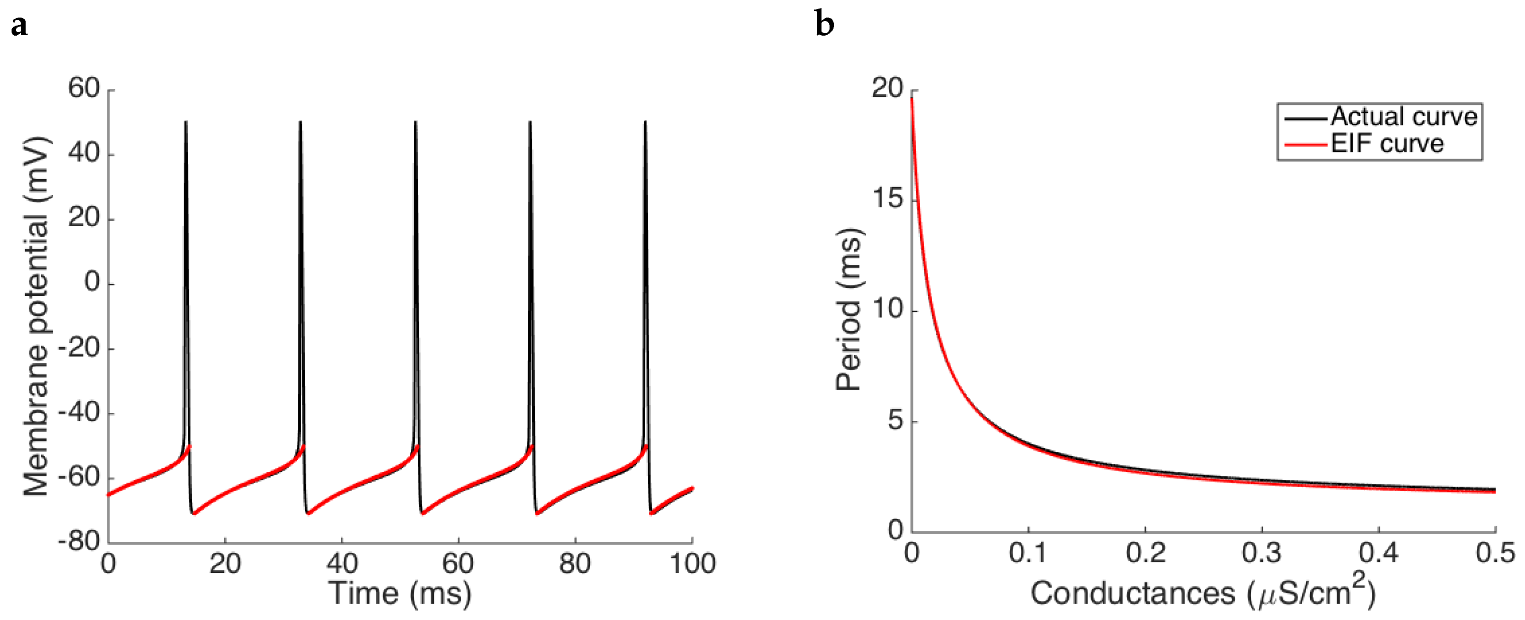
3.1.3. Estimation When the Neural Model Is Approximated by a Base Model

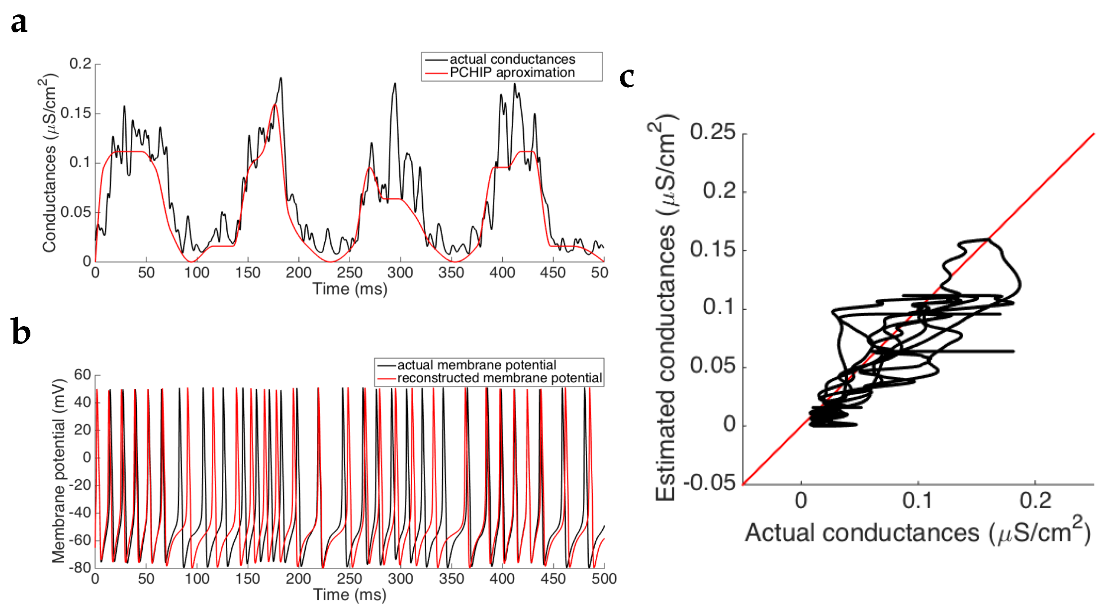
In many experimental cases, the exact model describing the target neuron is not known. One plausible way to apply our methodology is by fitting the measured data to a reference model. In this section, we explore this paradigm and study the errors of the estimation procedure. For this purpose, we generate membrane potential traces from the noisy pyramidal cell model (3) (see also Figure 2 in Section 2) with the synaptic drive shown in Figure 5a, and use them to fit an exponential integrate-and-fire model (5). The underlying assumption is that the fitted EIF model provides a good approximation of the original model (see Figure 2).

In order to challenge our methodology, we consider the worst scenario regarding data discretization and noise levels according to our previous results (see Table 2 and Table 3): we assume a discretization step size for the conductances (${\delta }_g={10}^{-3}$) and a high standard deviation for the white noise in the membrane potential (${\sigma }_V=0.1$ mV). Even so, results still show a good performance of the estimation procedure, see Figure 5, unexpectedly similar to the results obtained in Section 3.1.1.

As we can see in Figure 5a, some of the small oscillations are tracked properly, yielding to some temporal shifts on the onset of spikes when reconstructing the membrane potential (see Figure 5b). However, despite of this loss, the estimation keeps capturing the spiking frequency, and the conductances are estimated with a relative error of $2.7\%$ (mean over time) whereas the MSE is $7.038\times {10}^{-7}$. After interpolating the data, the relative error drops to $1.45\%$ and the MSE is equal to $7.348\times {10}^{-7}$. Note that the difference between these errors and those provided by the same case when we use the exact neural model in the estimation procedure does not differ qualitatively (see the first two rows of

Table 4. Errors caused by the computation of the $\mathit{T}-{\mathit{g}}_{\mathit{syn}}$ curve. Data are generated using the pyramidal cell model and adding noise to the voltage trace derivative (mean 0 and ${\sigma }_V=0.1$). The errors shown in the table correspond to the difference between the original synaptic trace and the estimated one (both before and after interpolating the estimated values) by using the corresponding base model.

Used	Mean of	MSE	MSE	Estimation of the
Base	the Relative	Estimated	Interpolated	Interpolated Mean
Model	Error	Values	Values	(Rel. Error)
Pyramidal	$2.667\times {10}^{-2}$	$9.419\times {10}^{-7}$	$9.726\times {10}^{-7}$	$1.637\times {10}^{-2}$
EIF (table)	$2.700\times {10}^{-2}$	$7.038\times {10}^{-7}$	$7.348\times {10}^{-7}$	$1.450\times {10}^{-2}$
EIF (expression)	$1.730\times {10}^{-2}$	$2.680\times {10}^{-7}$	$3.480\times {10}^{-7}$	$2.190\times {10}^{-3}$
Exper. curve	$3.821\times {10}^{-2}$	$9.822\times {10}^{-7}$	$1.146\times {10}^{-6}$	$3.827\times {10}^{-2}$

). Therefore, even though we assume that the exact model is not known, we still obtain good estimates of the time course of the synaptic conductance extracting the $T-g_{syn}$ relationship from an approximated base model (EIF in this case).

In the estimation procedure we have built a conductances’ table to be able to make the estimation. However, note that for this specific case, and when the conductances are supposed to be constant, there exists a closed expression for the EIF period, $T_{EIF}\left(g_{syn}\right)$, see Equation (6). This fact allows us to replace the table of the estimation procedure for the solution $T_{EIF}\left(g_{syn}\right)=T^{*}$, where $T^{*}$ is the specific interspike considered in each iteration of the procedure. Knowledge of this expression allows us to estimate the conductances more efficiently and with less numerical errors (see third row in Table 4).

3.1.4. Estimation without a Reference Base Model

To fully explore all possibilities of how to extract a relation between the oscillatory period and a constant value of the conductance, apart from considering an approximate model from which we can build up a table or find an explicit expression, we also consider the possibility of having the $T-g_{syn}$ relationship experimentally. This relationship could be directly obtained by using the dynamic clamp technique or indirectly through the $I-V$ curve by using other techniques (such as current clamp). Indeed, if the current I only contains synaptic currents, then the $T-g_{syn}$ curve can be obtained by computing $g_{syn}=\frac{I}{V-V_{syn}}$ and extracting the period T from the membrane potential trance.

Note that, if the $T-g_{syn}$ curve can be obtained with high accuracy (with a sufficiently fine discretization of points), then the estimation will present similar errors than those presented in Section 3.1 (see Table 2). However, if the discretization is poor, errors could be magnified.

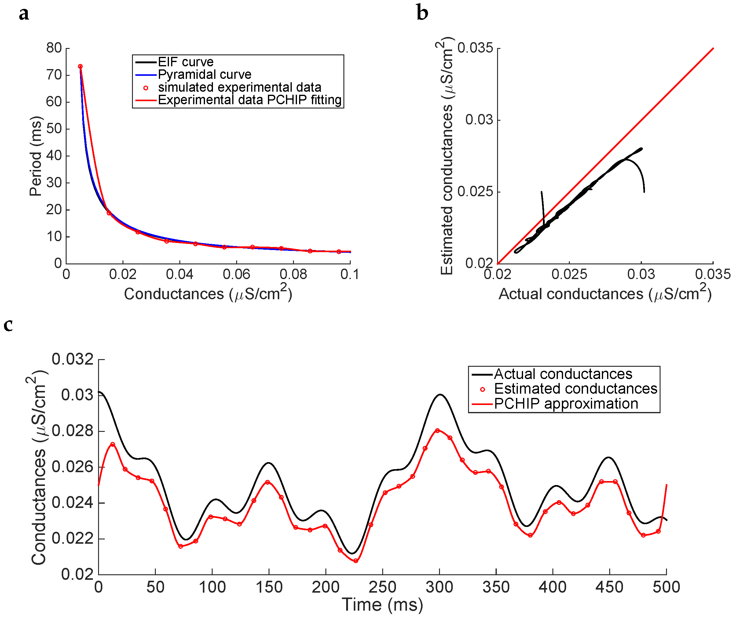
In this section, we investigate the case where only a small sample of $(g_{syn},T\left(g_{syn}\right))$ pairs are obtained. To computationally simulate this specific situation, we assume that the data set is generated from the noisy pyramidal cell model. By using this same model, we generate a small sample of ten $(g_{syn},T\left(g_{syn}\right))$ pairs to construct the $T-g_{syn}$ curve. Moreover, to consider possible errors in the recordings (measurement noise and variability across trials), we have added noise to the resulting set of points. This bias has been included by adding a random normal distributed value with 0 mean and 0.5 standard deviation to the period component. Finally, to estimate the conductance for any given period, and as we are supposing that no extra information is known about the actual data, we have interpolated these data using the PCHIP method (see Figure 6a).

Applying now the estimation procedure to the membrane potential shown in Figure 3b (black trace), using the simulated experimental curve instead of an approximate base model to generate the $T-g_{syn}$ curve, the results show how the estimated conductances are clearly underestimated (see Figure 6b,c) and, even though the frequency of oscillation of conductances is maintained, the amplitude of the oscillation is reduced. This fact is mainly due to misestimations that arise in the $T-g_{syn}$ experimentally fitted curve (with respect to that obtained with the actual model), specially the underestimation obtained for those values of conductances between $0.02$ and $0.04$, which is in fact the interval where the actual conductances lie.

However, in view of the magnitude of the conductances, these underestimations are not substantially significant, providing similar errors to the cases where the $T-g_{syn}$ curve is numerically computed from a base model (see fourth row in Table 4).

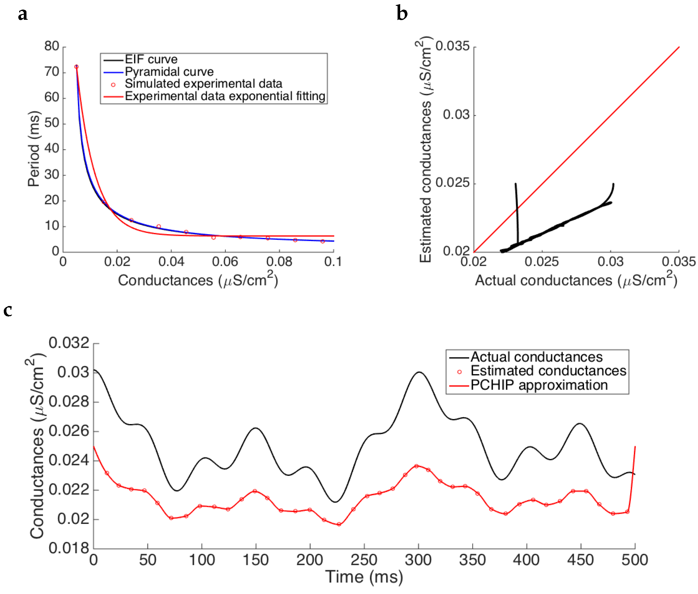
Note that the errors in the $T-g_{syn}$ curve can alter consistently the overall estimation causing an important increase of the errors in the estimation. One source of these misestimations is the interpolation method. We also tested an exponential fitting, instead of the PCHIP interpolation, which gave us higher misestimations of the $T-g_{syn}$ curve in the working interval, see Figure 7. Results show, as previously, that the frequency of oscillation is maintained but the amplitude is worst underestimated providing an average relative error of approximately $15\%$. Therefore, the errors are substantially magnified showing the importance of having a good approximation of the $T-g_{syn}$ curve to be able to properly estimate the conductances.

3.2. Estimation in the Spiking Regime with Interspersed Short Subthreshold Periods

In this section, we aim to explore whether the estimation procedure can be also used when short periods of subthreshold activity interrupt the spiking regime. Note that, if those silent periods are sufficiently large (for instance, greater than 100 ms), one could use a combination of the spiking estimation procedure developed in Section 2.2 and a subthreshold estimation procedure (for instance, the so-called QIF method presented in [23], which takes into account the spike initialization and possible subthreshold activity). However, for shorter subthreshold regimes, this combination could be not possible (as some methods require a certain amount of data to be used) or could cause a lot of misestimations induced by recent spike activity. 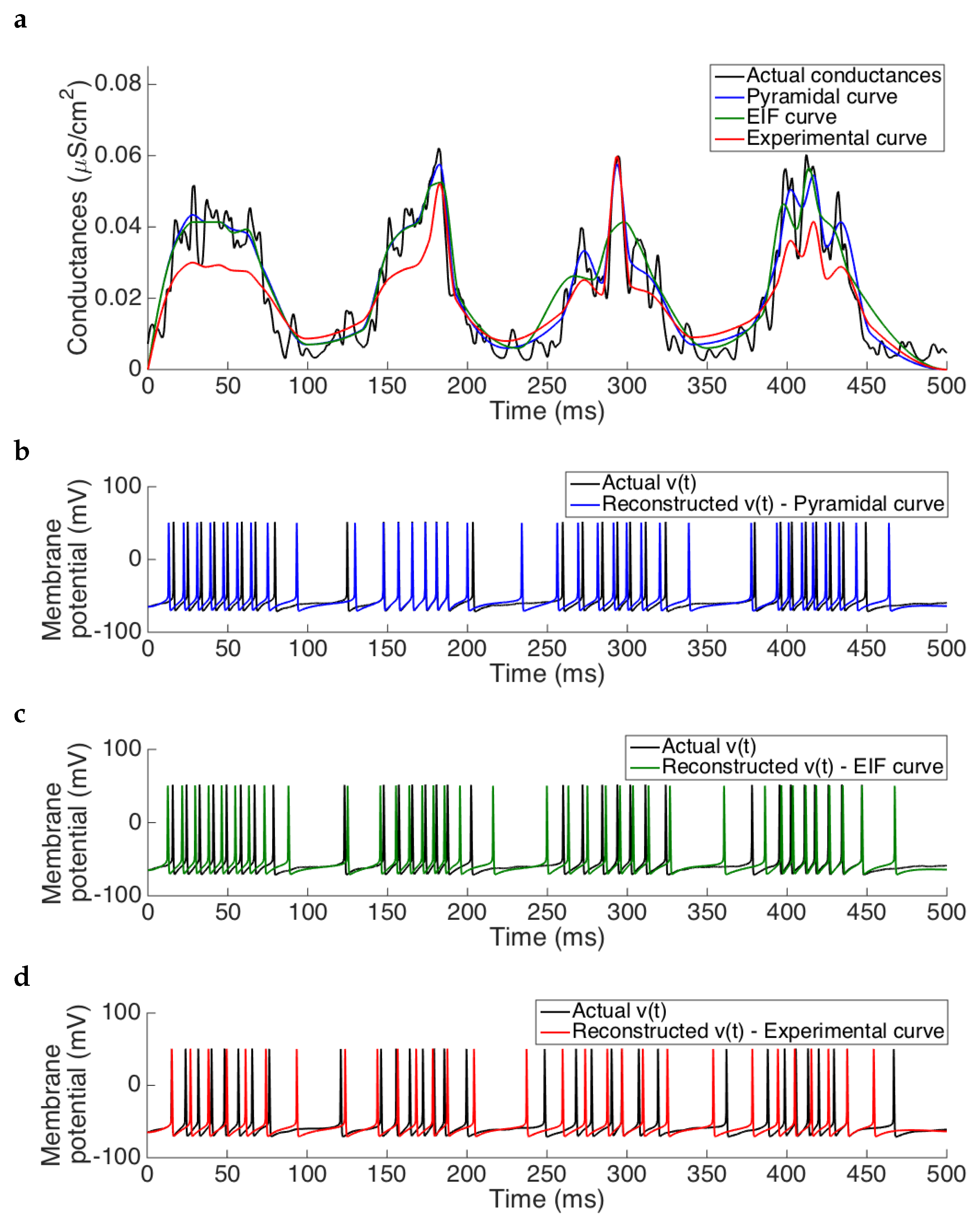For these reasons, we consider a synaptic conductance trace (see Section 2.1.2), depicted in Figure 8a (black trace), which causes spiking regimes interleaved with subthreshold regimes (of 50 ms of duration, approximately) when this is used into the pyramidal cell model (see Figure 8b (black trace)).

Results presented in Figure 8a show that the estimation procedure provided in Algorithm 1 is able to reproduce the synaptic drive, either if we use as a base model to generate the $T-g_{syn}$ table the pyramidal cell model (blue trace) or the EIF model (green curve). In both cases, the reconstruction of the membrane potential using the estimated conductances maintains the spike frequency, thus keeping unchanged the firing rate (Figure 8b,c, respectively). On the other hand, when the simulated experimental curve is used, conductances around $[0.02,0.04]$ are not well estimated, as it happened when considering just the spiking regime, see Section 3.1.4. These misestimates alter the spike frequency in the membrane potential reconstructed using the estimated conductances as synaptic inputs (see Figure 8b), by adding extra spikes in the silent regime and displacing the spiking time-onset in the spiking regime.

Errors of the estimation in the different cases are presented in

Table 5. Errors caused by the computation of the $\mathit{T}-{\mathit{g}}_{\mathit{syn}}$ curve. Data have been generated using the pyramidal cell model with noise (mean 0 and ${\sigma }_V=0.1$). The synaptic drive is governed by a synaptic conductance trace extracted from an in silico network (see end of Section 2.1.2) where we have added noise with mean 0 and $\sigma =0.0001$ (see Figure 4a, black curve).

	Mean of	MSE	MSE	Estimation of the
Base	the Relative	Estimated	Interpolated	Interpolated Mean
Model	Error	Values	Values	(Rel. Error)
Pyramidal	$7.820\times {10}^{-2}$	$1.491\times {10}^{-5}$	$3.776\times {10}^{-5}$	$8.105\times {10}^{-2}$
EIF	$8.768\times {10}^{-2}$	$2.303\times {10}^{-5}$	$3.576\times {10}^{-5}$	$7.331\times {10}^{-2}$
Exper. curve	$3.001\times {10}^{-1}$	$1.334\times {10}^{-4}$	$7.171\times {10}^{-5}$	$1.215\times {10}^{-1}$

, where we can see also that both the pyramidal cell model and its EIF approximation lead to similar errors, while the experimental curve leads to higher errors.

4. Discussion

Estimations of the time course of synaptic conductances arriving at a single cell (or a population) reveal relevant information to fully understand the functional connectivity of the brain. Several strategies have been developed for the estimation during subthreshold activity regimes [3,4,5,6,7,8,9,10,12,13,14,15,16,17,18,19,21,22,23,25]. However, the estimation during oscillatory (spiking) regimes has received less attention [25,26,27,40]. The main drawback is the predominance of ionic currents over synaptic ones in this regime. Nevertheless, as we already showed in a caricature model (see [26]), if one gets the main information about the contribution of ionic currents and is able to track their activity during the spiking regime, then it is possible to infer the synaptic activity. In this paper, we extend this idea to more realistic spiking models and provide a systematic procedure that can be applied to a variety of neural data, coming both from computational simulations and from experiments. The idea is to exploit the input-response properties of the cell; more precisely, the relation between constant synaptic conductances and the spiking frequency (the $f-g_{syn}$ curve).

In the spiking regime, the most natural measurable quantity is the oscillation frequency, which constitutes a valuable piece of information for our purpose. The frequency–input relationship encompasses the average response of the neuron, which includes both the direct effect of the input stimulus and the resulting activation of ionic currents. The fact that $f-I$ curves are usually monotone implies the one-to-one correspondence between frequency and input, and favors the resolution of the inverse problem. However, while in the case of a steady input (I constant) that induces a constant-frequency repetitive firing, it is straightforward to infer the input current from the output frequency; the presence of the neuron’s voltage in the synaptic current ($I=g_{syn}\left(t\right)(v\left(t\right)-V_{syn})$ in their minimal expression) makes the estimation of the total input current highly sensitive to the fluctuations in $g_{syn}$. Here, we propose to consider an alternative frequency–input relationship, the $f-g_{syn}$ curve, which is more appropriate for the estimation problem since it implicitly incorporates the voltage dependency of the synaptic current and mitigates the effects of the fluctuations. In a mathematical model, we can obtain the $f-g_{syn}$ or $T-g_{syn}$ curve, $T=1/f$, numerically (in some cases, even analytically or quasi-analytically, see [26] and Section 2.1.1). For experimental studies, retrieving the $T-g_{syn}$ curve requires the use of dynamic clamp techniques on the isolated cell for fixed $g_{syn}$ values within a physiologically plausible interval. In Algorithm 1, we summarize the steps to perform the estimation of synaptic conductances from the interspike intervals of the voltage traces and the knowledge of the $T-g_{syn}$ curve.

The second ingredient of the method presented in this paper is the choice of a reference/base model, which must be both flexible to fit to a variety of neural data (choosing a suitable parameter set in each case) and simple enough to be able to compute the $f-g_{syn}$ curve in a precise way. We found the exponential integrate-and-fire model (EIF) to be a convenient base model: on the one hand, its oscillation period can be well approximated by means of the semi-analytical formula (6); on the other, there are examples in the literature showing that its $f-I$ curve can fit $f-I$ curves of neural data.

Our procedure has been applied first to a representative computational model driven by a prescribed input conductance trace. We verify that the use of the $f-g_{syn}$ curve brings excellent predictions of the $g_{syn}$ fluctuations along the prescribed trace, see Figure 3. We also observe better estimations when the synaptic conductances change on a time-scale longer than the mean interspike interval. We also analyze the effects of the discretization and the measurement noise, see Table 2 and Table 3. In particular, we observe that levels of noise below 1 mV do not compromise the estimations in a substantial way since the MSE of the estimations is very low (MSE $<{10}^{-6}$) in all cases. In Section 3.1.3, we explore the goodness of the estimations under the assumption that the EIF (base) model provides a good fit to the neural data. By using a model for a noisy pyramidal cell to generate the data, we again observe excellent estimations of the synaptic conductance (MSE $<{10}^{-6}$), see Figure 5. We conclude that we could reasonably estimate the synaptic conductances from other neural data to which the EIF could be fitted.

We next study potential difficulties that can be found in more realistic scenarios. First, in Section 3.1.4, we cope with the problem of estimating synaptic conductances when there is no base model that decently fits the data. We propose a procedure to come up with an approximation of the $T-g_{syn}$ curve and apply it to data generated by a computational model. Again, we achieve good estimations (MSE $<{10}^{-6}$), see Table 4. For real cells, the dynamic-clamp technique allows obtaining the period T from a $g_{syn}$ value, and therefore it would be interesting to design a protocol so that it was feasible to obtain the $T-g_{syn}$ curve. As our method is mainly addressed to the spiking regime, the second potential difficulty is the presence of interspersed short subthreshold periods. We show (see Figure 8) that these short subthreshold periods do not contaminate the estimation of synaptic conductances and provide results with small errors.

In order to check the robustness of the estimation procedure for other types of neurons, we have also considered the stellate cell model (see Section 3.1.2), to which the quadratic integrate and fire model (QIF; see [30]) has been fitted. Results (not shown) reveal that the estimation procedure can also be used in cases where the fitting is not as perfect as those obtained for the pyramidal cell model.

Our method is related in spirit to the firing-clamp method presented in [25], where the authors also consider a point neuron and, by calibrating its activity, they experimentally build up an approximated function to describe the changes in both the membrane potential threshold and the amplitude of the spiking regime (instead of the spiking frequency). Their model is able to discern between excitatory and inhibitory conductances; however, as their calibration is purely experimental, errors could arise from the measurement noise because of repetitive trials.

5. Conclusions

Estimation of synaptic conductances from the time course of a neuron’s membrane potential is a challenging inverse mathematical problem, with strong implications in the study of the brain’s functional activity. Few methods are known that address the problem when the neuron is spiking. The aim of our research is building up a general method to estimate synaptic conductances based on the knowledge of the frequency versus synaptic conductance curve ($f-g_{syn}$). This strategy is complemented with the choice of a mathematical model for which the $f-g_{syn}$ curve can be accurately computed and, simultaneously, can fit a variety of data sources. We have shown that the exponential integrate-and-fire model (EIF) fulfills these requirements and can be a good reference model for future applications.

We have successfully applied the method to data generated from mathematical neuron models driven by different synaptic input profiles. We have tested different levels of knowledge of the $f-g_{syn}$ curve, namely, directly obtained from the neuron model, using the $f-g_{syn}$ curve corresponding to the base model and assuming no model behind. Of course, the latter gives the worst results, but still within high accuracy. The method has also proven to be robust under normal levels of measurement noise and alternation of spiking and subthreshold activity.

These results allow us to be optimistic about the application of the proposed methodology to obtain trustable estimations of the time course of synaptic conductance from real membrane potential traces presenting heterogeneous activity (combining subthreshold activity with intervals of spiking). Therefore, the next challenge is to discern between the excitatory ($g_{exc}$) and inhibitory ($g_{inh}$) conductances, which is relevant to understand how brain activity results from the interaction of different types of neurotransmission. For this purpose, one needs additional (uncorrelated) measurable quantities to build up a one-to-one relationship between pairs of measurable elements and the two parameters $g_{exc}$ and $g_{inh}$. Following the ideas in [25], we think that the amplitude of the spikes is a potential candidate as it is easily measurable and typically highly uncorrelated with the frequency.

References

1. McLaughlin, D.; Shapley, R.; Shelley, M.; Wielaard, D.J. A neuronal network model of macaque primary visual cortex (V1): Orientation selectivity and dynamics in the input layer 4Calpha. Proc. Natl. Acad. Sci. USA 2000, 97, 8087–8092. [Google Scholar] [CrossRef] [Green Version]
2. Destexhe, A.; Rudolph, M.; Paré, D. The high-conductance state of neocortical neurons in vivo. Nat. Rev. Neurosci. 2003, 4, 739–751. [Google Scholar] [CrossRef] [PubMed]
3. Wehr, M.; Zador, A.M. Balanced inhibition underlies tuning and sharpens spike timing in auditory cortex. Nature 2003, 426, 442–446. [Google Scholar] [CrossRef] [PubMed]
4. Borg-Graham, L.; Monier, C.; Frégnac, Y. Visual input evokes transient and strong shunting inhibition in visual cortical neurons. Nature 1998, 393, 369–373. [Google Scholar] [CrossRef] [PubMed]
5. Anderson, J.S.; Carandini, M.; Ferster, D. Orientation tuning of input conductance, excitation, and inhibition in cat primary visual cortex. J. Neurophysiol. 2000, 84, 909–926. [Google Scholar] [CrossRef] [Green Version]
6. Bédard, C.; Béhuret, S.; Deleuze, C.; Bal, T.; Destexhe, A. Oversampling method to extract excitatory and inhibitory conductances from single-trial membrane potential recordings. J. Neurosci. Methods 2011. [Google Scholar] [CrossRef]
7. Yasar, T.B.; Wright, N.C.; Wessel, R. Inferring presynaptic population spiking from single-trial membrane potential recordings. J. Neurosci. Methods 2016, 259, 13–21. [Google Scholar] [CrossRef]
8. Rudolph, M.; Piwkowska, Z.; Badoual, M.; Bal, T.; Destexhe, A. A Method to Estimate Synaptic Conductances From Membrane Potential Fluctuations. J. Neurophysiol. 2004, 91, 2884–2896. [Google Scholar] [CrossRef] [PubMed] [Green Version]
9. Pospischil, M.; Piwkowska, Z.; Bal, T.; Destexhe, A. Extracting synaptic conductances from single membrane potential traces. Neuroscience 2009, 158, 545–552. [Google Scholar] [CrossRef] [PubMed] [Green Version]
10. Paninski, L.; Vidne, M.; DePasquale, B.; Ferreira, D.G. Inferring synaptic inputs given a noisy voltage trace via sequential Monte Carlo methods. J. Comput. Neurosci. 2012, 33, 1–19. [Google Scholar] [CrossRef]
11. Odom, S.E.; Borisyuk, A. Estimating three synaptic conductances in a stochastic neural model. J. Comput. Neurosci. 2012, 33, 191–205. [Google Scholar] [CrossRef] [PubMed]
12. Berg, R.W.; Ditlevsen, S. Synaptic inhibition and excitation estimated via the time constant of membrane potential fluctuations. J. Neurophysiol. 2013, 110, 1021–1034. [Google Scholar] [CrossRef] [PubMed] [Green Version]
13. Kobayashi, R.; Nishimaru, H.; Nishijo, H. Estimation of excitatory and inhibitory synaptic conductance variations in motoneurons during locomotor-like rhythmic activity. Neuroscience 2016, 335, 72–81. [Google Scholar] [CrossRef] [PubMed]
14. Lankarany, M.; Zhu, W.P.; Swamy, M.N.S.; Toyoizumi, T. Inferring trial-to-trial excitatory and inhibitory synaptic inputs from membrane potential using Gaussian mixture Kalman filtering. Front. Comput. Neurosci. 2013, 7. [Google Scholar] [CrossRef] [PubMed] [Green Version]
15. Ditlevsen, S.; Samson, A. Estimation in the partially observed stochastic Morris-Lecar neuronal model with particle filter and stochastic approximation methods. Ann. Appl. Stat. 2014, 8, 674–702. [Google Scholar] [CrossRef]
16. Closas, P. Sequential Estimation of Neural Models by Bayesian Filtering. Master’s Thesis, FME-Univ. Politènica de Catalunya, Barcelona, Spain, 2014. [Google Scholar]
17. Lankarany, M.; Zhu, W.P.; Swamy, M. Joint estimation of states and parameters of Hodgkin-Huxley neuronal model using Kalman filtering. Neurocomputing 2014, 136, 289–299. [Google Scholar] [CrossRef]
18. Lankarany, M.; Heiss, J.E.; Lampl, I.; Toyoizumi, T. Simultaneous Bayesian Estimation of Excitatory and Inhibitory Synaptic Conductances by Exploiting Multiple Recorded Trials. Front. Comput. Neurosci. 2016, 10, 110. [Google Scholar] [CrossRef] [Green Version]
19. Li, S.; Liu, N.; Yao, L.; Zhang, X.; Zhou, D.; Cai, D. Determination of effective synaptic conductances using somatic voltage clamp. PLoS Comput. Biol. 2019, 15, 1–28. [Google Scholar] [CrossRef] [Green Version]
20. Guillamon, A.; McLaughlin, D.W.; Rinzel, J. Estimation of synaptic conductances. J. Physiol. Paris 2006, 100, 31–42. [Google Scholar] [CrossRef] [PubMed] [Green Version]
21. Kobayashi, R.; Nishimaru, H.; Nishijo, H.; Lansky, P. A single spike deteriorates synaptic conductance estimation. Biosystems 2017, 161, 41–45. [Google Scholar] [CrossRef]
22. Vich, C.; Guillamon, A. Dissecting estimation of conductances in subthreshold regimes. J. Comput. Neurosci. 2015, 1–17. [Google Scholar] [CrossRef] [PubMed] [Green Version]
23. Vich, C.; Berg, R.; Guillamon, A.; Ditlevsen, S. Estimation of synaptic conductances in presence of nonlinear effects caused by subthreshold ionic currents. Front. Comput. Neurosci. 2017, 11, 69. [Google Scholar] [CrossRef] [PubMed] [Green Version]
24. Chizhov, A.V.; Amakhin, D.V. Method of experimental synaptic conductance estimation: Limitations of the basic approach and extension to voltage-dependent conductances. Neurocomputing 2018, 275, 2414–2425. [Google Scholar] [CrossRef]
25. Chizhov, A.; Malinina, E.; Druzin, M.; Graham, L.J.; Johansson, S. Firing clamp: A novel method for single-trial estimation of excitatory and inhibitory synaptic neuronal conductances. Front. Cell. Neurosci. 2014, 8. [Google Scholar] [CrossRef]
26. Guillamon, A.; Prohens, R.; Teruel, A.; Vich, C. Estimation of synaptic conductances in the spiking regime for the McKean neuron model. SIAM J. Appl. Dyn. Syst. 2017, 16, 1397–1424. [Google Scholar] [CrossRef] [Green Version]
27. Lankarany, M. Estimating Excitatory and Inhibitory Synaptic Conductances from Spike Trains using a Recursive Bayesian Approach. bioRxiv 2017. [Google Scholar] [CrossRef] [Green Version]
28. Wang, X.J. Calcium coding and adaptive temporal computation in cortical pyramidal neurons. J. Neurophysiol. 1998, 79, 1549–1566. [Google Scholar] [CrossRef]
29. Rotstein, H.; Oppermann, T.; White, J.; Kopell, N. The dynamic structure underlying subthreshold oscillatory activity and the onset of spikes in a model of medial entorhinal cortex stellate cells. J. Comput. Neurosci. 2006, 21, 271–292. [Google Scholar] [CrossRef]
30. Fourcaud-Trocmé, N.; Hansel, D.; van Vreeswijk, C.; Brunel, N. How spike generation mechanisms determine the neuronal response to fluctuating inputs. J. Neurosci. 2003, 23, 11628–11640. [Google Scholar] [CrossRef]
31. Izhikevich, E.M. Simple model of spiking neurons. IEEE Trans. Neural Netw. 2003, 14, 1569–1572. [Google Scholar] [CrossRef] [Green Version]
32. Pospischil, M.; Piwkowska, Z.; Bal, T.; Destexhe, A. Comparison of different neuron models to conductance-based post-stimulus time histograms obtained in cortical pyramidal cells using dynamic-clamp in vitro. Biol. Cybern. 2011, 105, 167. [Google Scholar] [CrossRef] [PubMed]
33. Rossant, C.; Goodman, D.; Platkiewicz, J.; Brette, R. Automatic fitting of spiking neuron models to electrophysiological recordings. Front. Neuroinform. 2010, 4, 2. [Google Scholar] [CrossRef] [PubMed] [Green Version]
34. Daneshzand, M.; Faezipour, M.; Barkana, B.D. Hyperbolic modeling of subthalamic nucleus cells to investigate the effect of dopamine depletion. Comput. Intell. Neurosci. 2017, 2017. [Google Scholar] [CrossRef] [PubMed] [Green Version]
35. Badel, L.; Lefort, S.; Brette, R.; Petersen, C.C.H.; Gerstner, W.; Richardson, M.J.E. Dynamic I-V Curves Are Reliable Predictors of Naturalistic Pyramidal-Neuron Voltage Traces. J. Neurophysiol. 2008, 99, 656–666. [Google Scholar] [CrossRef] [Green Version]
36. Badel, L.; Lefort, S.; Berger, T.K.; Petersen, C.C.H.; Gerstner, W.; Richardson, M.J.E. Extracting non-linear integrate-and-fire models from experimental data using dynamic I–V curves. Biol. Cybern. 2008, 99, 361. [Google Scholar] [CrossRef] [Green Version]
37. Gerstner, W.; Kistler, W.M.; Naud, R.; Paninski, L. Nonlinear integrate-and-fire models. In Neuronal Dynamics: From Single Neurons to Networks and Models of Cognition; Cambridge University Press: Cambridge, UK, 2014; pp. 119–135. [Google Scholar] [CrossRef]
38. Tao, L.; Shelley, M.; McLaughlin, D.; Shapley, R. An egalitarian network model for the emergence of simple and complex cells in visual cortex. Proc. Natl. Acad. Sci. USA 2004, 101, 366–371. [Google Scholar] [CrossRef] [Green Version]
39. Burden, R.; Faires, J. Numerical Analysis; Available Titles CengageNOW Series; Cengage Learning: Belmont, CA, USA, 2004. [Google Scholar]
40. Closas, P.; Guillamon, A. Sequential estimation of intrinsic activity and synaptic input in single neurons by particle filtering with optimal importance density. EURASIP J. Adv. Signal Process. 2017, 2017. [Google Scholar] [CrossRef] [Green Version]
Figure 2. Approximation of the pyramidal cell model by the EIF model. Panel (a) shows the membrane potential trace obtained from the pyramidal cell model (black curve) given in Equation (1) when no synaptic input is considered, and the approximation of the membrane potential trace obtained by the EIF model (red curve) described in Equation (5). Panel (b) shows their respective T g s y n curve, where T is the period of oscillation (the black curve corresponds to the pyramidal case and the red curve to the EIF model).
Mathematics 08 02153 g002
Figure 3. Results of the estimation procedure applied to a membrane potential generated through the pyramidal cell model with no additive noise, and using this same model as a base model in the estimation procedure. Panel (a) shows the prescribed conductances (black curve) and the estimated conductances (red curve). Panel (b) shows the membrane potential (black curve) obtained from the pyramidal cell model described in Section 2.1.1 and using the prescribed conductances of panel (a), and the reconstructed membrane potential (red curve) obtained also from the pyramidal cell model described in Section 2.1.1 but using the estimated conductances. Panel (c) shows the scatter plot of the prescribed conductances versus the estimated ones. The red line represents the identity line.
Mathematics 08 02153 g003
Figure 4. Results of the estimation procedure for a membrane potential from a stellate cell model using the same model as a base model in the estimation procedure. Panel (a) shows the prescribed conductances (black curve) and the estimated conductances (red curve). Panel (b) shows the membrane potential (black curve), obtained from the stellate cell model described in (4) when the prescribed conductances of Panel (a) has been used, while the red curve depicts for the reconstructed membrane potential, obtained also from the stellate cell model but using the estimated conductances. Panel (c) shows the scatter plot of the prescribed conductances versus the estimated ones. The red line represents the identity line.
Mathematics 08 02153 g004
Figure 5. Results of the conductance estimation applied to a membrane potential generated from the noisy pyramidal cell model, but using the EIF model as a base model in the estimation procedure. Panel (a) shows the prescribed conductances (black curve) and the estimated conductances (red curve). Panel (b) shows the membrane potential (black curve) obtained from the noisy pyramidal cell model (3) with σ V = 0.1 and using the prescribed conductances of panel (a), and the reconstructed membrane potential (red curve) obtained also from the noisy pyramidal cell model but using the estimated conductances as input. Panel (c) shows the scatter plot of the prescribed conductances versus the estimated ones. The red line represents the identity line.
Mathematics 08 02153 g005
Figure 6. Results of the estimation procedure applied to a membrane potential generated through the pyramidal cell model with additive noise, and using a simulated T g syn curve in the estimation procedure. Panel (a) shows the actual T g s y n curve (blue curve), the T g s y n curve obtained with the EIF method (black curve), a simulation of an experimental T g s y n curve (red dots), and an exponential fitting of the experimental curve (red curve). Panel (b) shows the scatter plot of the prescribed conductances versus the estimated ones; the red line represents the identity line. Panel (c) shows the prescribed conductances (black curve) and the estimated conductances (red curve). In panel (a), the experimental curve (red dots) has been computed using 10 different trials where noise has been added to the period (a random normal distributed value with 0 mean and 0.5 standard deviation) and the interpolated using the PCHIP method.
Mathematics 08 02153 g006
Figure 7. Results of the estimation procedure applied to a membrane potential generated through the pyramidal cell model with additive noise and using a simulated T g syn curve in the estimation procedure. Panel (a) shows the actual T g s y n curve (blue curve), the T g s y n curve obtained with the EIF method (black curve), a simulation of an experimental T g s y n curve (red dots), and an exponential fitting of the experimental curve (red curve). Panel (b) shows the scatter plot of the prescribed conductances versus the estimated ones; the red line represents the identity line. Panel (c) shows the prescribed conductances (black curve) and the estimated conductances (red curve). In panel (a), the experimental curve (red dots) has been computed using 10 different trials where noise has been added to the period (a random normal distributed value with 0 mean and 0.5 standard deviation and dots has been interpolated using the exponential fitting).
Mathematics 08 02153 g007
Figure 8. Results of the estimation procedure applied to a non-tonic membrane potential from a noisy pyramidal cell model. Panel (a) shows the prescribed conductances (black curve) and the estimated conductances using the same model (blue trace), the EIF model (green trace), and the experimentally fitted curve (red trace). Panels (bd) show the reconstructed membrane potential when each of the mentioned estimated conductances in panel (a) has been, respectively, used as input to the base model (the noisy pyramidal cell model).
Mathematics 08 02153 g008