Accumulative Pension Schemes with Various Decrement Factors

Abstract

We consider accumulative defined contribution pension schemes with a lump sum payment on retirement. These schemes differ in relation to inheritance and provide various decrement factors. For each scheme, we construct the balance equation and obtain an expression for calculation of gross premium. Payments are made at the end of the insurance event period (survival to retirement age or death or retirement for disability within the accumulation interval). A simulation model was developed to analyze the constructed schemes.

1. Introduction

At present, the accumulative pension schemes with a lump sum payment are not used in the Russian Federation. Such schemes may be of interest to many people for many reasons. For example, the pensioner plans to make large purchases, such as purchase of housing, purchase of household appliances and/or purchase of expensive treatment. In addition, such schemes allow elderly parents to ensure the future of their minor children.

At the end of October 2019, the Central Bank and the Ministry of Finance of the Russian Federation announced a draft law for a new system of voluntary retirement savings, called Guaranteed Retirement Plan. This draft law inspired the authors to write this article.

Pension schemes with the possibility of inheritance are popular in many countries. For example, in the United Kingdom, in many circumstances, one can inherit a pension. Examples of such pension schemes are defined contribution pension funds, joint life annuities and annuities with guarantee periods. In the UK, it has now become easier to inherit a pension thanks to the 2015 pension freedoms and the introduction of flexi-access drawdown, which is a newer, more flexible version of pension drawdown (see [1,2,3,4]).

In this work, we used standard methods of actuarial calculations. However, the authors would like to emphasize that since the actuarial calculations associated with a specific insurance contract are made by the actuaries of the insurance companies and pension funds; the details of these calculations are confidential.

Let us now describe the main results of this work. In this work, we consider accumulative defined contribution pension schemes with a lump sum payment on retirement. These schemes differ in relation to inheritance and provide various decrement factors: mortality or mortality and disability (recall that the disability retirement is a plan of retirement which is invoked when person covered is disabled from working to normal retirement age). It is assumed that contributions are paid regularly at the beginning of each period (monthly, quarterly, yearly, etc.). In other words, the contributions (without premium load) form an annuity due (for more details about basic actuarial definitions and terminology, see [5,6]). Recall that the premium load is a percentage of insurance premium deducted from the premium payments to cover policy administrative expenses, including the agent’s sales commissions and a return on investment.

For each scheme, we construct the balance equation and obtain an expression for calculation of gross premium (Propositions 1–4). The balance equation is based on the equivalence principle of financial liabilities of the pension fund and the insured person. In general, the equivalence principle states that the (expected) present values of premiums and benefits should be equal. In other words, the equivalence principle ensures that, at any time, the net contributions (i.e., the contributions balance after taking into account the premium load) in the past provide precisely the amount needed to meet net liabilities in the future. Note that the premium load leads to a decrease of contributions when applying the principle of equivalence.

For all schemes with the possibility of inheritance (see Section 2.2, Section 2.3 and Section 3), we assume that if the death or disability of the insured person occurs before reaching the retirement age then the payments will be made not at the time of death or disability, but at the end of the last contribution period in which the death or disability occurs (in other words, we consider the so-called discrete models of pension insurance). It is assumed that the net contributions are not refunded if the death occurs within the last period of the insurance contract. In the event of disability within the last period of the insurance contract, the insured receives the lump sum payment at the end of this period.

Note that for long-term insurance, the investment income of the collected premiums should be taken into account in the balance equation. This income is related to the changing value of money over time. In particular, when deriving the balance equation, it is necessary to find the (present) value of liabilities of the pension fund and the insured person (i.e., the value of contributions and payments) relative to one time point [5,6]. For our schemes, we derive the balance equation relative to the moment of concluding the pension insurance contract.

To analyze the constructed schemes, in Section 4 we discuss the results of a simulation model developed by the authors for calculating the gross premium.

This work is dedicated to Zolotarev V.M. the founder of the International Seminar on Stability Problems for Stochastic Models and to Kalashnikov V.V., whose works have important applications in actuarial mathematics and mathematical risk theory (see [7,8,9,10,11]. See also [12]).

Some results of this work were announced in Russian in [13,14].

2. Cumulative Models of Pension Insurance Based on one Decrement Factor (Mortality)

In this section, we consider accumulative defined contribution pension schemes with a lump sum payment on retirement. These schemes differ in relation to inheritance and provide one decrement factor (mortality). It is assumed that contributions are paid regularly at the beginning of each period (monthly, quarterly, yearly, etc.).

In this section, we use the following notation:

• x is the age of the insured person at the time of concluding the pension insurance contract.
• y is the retirement age (for example, $y=55$, 60 or 65).
• B is the gross premium paid by the policyholder at the beginning of each period (monthly, quarterly, yearly, etc.) until retirement.
• $P_l$ is the lump sum payment on retirement if the insured person survives to the retirement age.
• ${\alpha }_1,\dots ,{\alpha }_{y-x}$ are the annual premium loads under the insurance pension contract.
• i is the effective annual interest rate, $\nu =\frac{1}{1+i}$ is the annual discount factor and $a=1+i$ is the annual growth rate.
• $P_r$ is the present value of the net contributions refunded to the inheritors if the insured dies before surviving to the retirement age. It is assumed that the net contributions are not refunded if the death occurs within the last period of the insurance contract.

Let us recall the definitions of some actuarial symbols (life table notation) that are used in this section (for more details see [5,6]).

With a starting group of $l_0$ newborns $l_z$ denotes the expected number of survivors at age z from the original group.

Some definitions and relationships involving life table functions are:

• $d_z=l_z-l_{z+1}$ is the number of deaths between ages z and $z+1$.
• The number of deaths between ages z and $z+t$ is

  $${}_t{d}_z=l_z-l_{z+t}.$$
  If $t=n$ is an integer, then

  $${}_n{d}_z=d_z+d_{z+1}+\dots +d_{z+n-1}.$$
  Note that ${}_1{d}_z=d_z$.
• The notation $\left(z\right)$ refers to an individual alive at age z.
• ${}_t{q}_z=\frac{{}_t{d}_z}{l_z}$ is the probability that $\left(z\right)$ will die within the next t years (by age $z+t$).
• The complement of ${}_t{q}_z$ is denoted by ${}_t{p}_z=1-{}_t{q}_z=\frac{l_{z+t}}{l_z}$ which is the probability that $\left(z\right)$ survives at least to time t (and dies some time after t).
• Recall that for discrete n-year temporary life annuity due the first payment (contribution) is made at age z and the latest possible payment is made at age $z+n-1$ (a maximum of n payments, with last occurring at the beginning of the n-th year). The actuarial present value of this annuity is denoted by ${\ddot{a}}_{z:\overline{n}|}$. We have (see [5,6]).

  $${\ddot{a}}_{z:\overline{n}|}=\sum _{k=0}^{n-1}{\nu }^k{}_k{p}_z.$$

2.1. Scheme 1. Accumulative Pension Scheme with Annual Contributions and a Lump Sum Payment on Retirement and without the Possibility of Inheritance

Consider an accumulative defined contribution pension scheme with a lump sum payment on retirement and without the possibility of inheritance (i.e., $P_r=0$). Suppose that a group of individuals at age x start to pay the pension contributions of size B at the beginning of each year until retirement, i.e., until the age y. A schematic drawing of this pension model is presented in Figure 1.

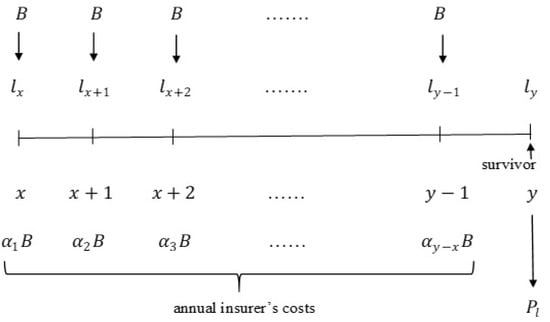
Figure 1. Schematic drawing of the accumulative pension scheme with annual contributions and a lump sum payment on retirement and without the possibility of inheritance.

Proposition 1.

Consider the pension Scheme 1. Then, the balance equation has the form

$$B{\ddot{a}}_{x:\overline{y-x}|}=B\sum _{k=0}^{y-x-1}{\alpha }_{k+1}{\nu }^k{}_k{p}_x+P_l{}_{y-x}{p}_x{\nu }^{y-x}.$$

(1)

In particular, the annual gross premium B is equal to

$$B=\frac{P_l{}_{y-x}{p}_x{\nu }^{y-x}}{{\ddot{a}}_{x:\overline{y-x}|}-{\displaystyle \sum _{k=0}^{y-x-1}}{\alpha }_{k+1}{\nu }^k{}_k{p}_x}.$$

(2)

The proof of Proposition 1 will be given in Section 2.3 as a special case of more general pension scheme (Scheme 3).

2.2. Scheme 2. Accumulative Pension Scheme with Annual Contributions and a Lump Sum Payment on Retirement and with Possibility of Inheritance

Consider Scheme 1 with possibility of inheritance. In other words, assume that if the insured dies before surviving to the retirement age, then all the net contributions are paid before the deaths are refunded to the inheritors at the end of the death year.

Recall that $P_r$ is the present value of the net contributions refunded to the inheritors and $P_l$ is the lump sum payment on retirement. Recall also that the net contributions are not refunded if the death occurs within the last period of the insurance contract (i.e., within $(y-1,y)$). A schematic drawing of this pension model is presented in Figure 2.

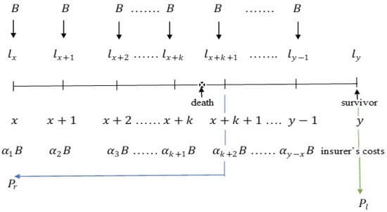
Figure 2. Schematic drawing of the accumulative pension scheme with annual contributions and a lump sum payment on retirement and with the possibility of inheritance.

Proposition 2.

Consider the pension Scheme 2. Then, the balance equation has the form

$$B{\ddot{a}}_{x:\overline{y-x}|}=B\sum _{k=0}^{y-x-1}{\alpha }_{k+1}{\nu }^k{}_k{p}_x+P_l{}_{y-x}{p}_x{\nu }^{y-x}+P_r^{\prime },$$

(3)

where

$$P_r^{\prime }=\frac{P_r}{l_x}=B\sum _{j=1}^{y-x-1}{}_{j-1|}{q}_x\sum _{k=1}^j(1-{\alpha }_k){\nu }^{k-1}$$

(4)

and

$${}_{s|}{q}_x=\frac{l_{x+s}-l_{x+s+1}}{l_x}$$

(5)

is the probability that $\left(x\right)$ will die in a year, deferred s years; that is, that he will die in the $(s+1)$th year (see [5,6] for more details about this actuarial symbol).

In particular, the annual gross premium B is equal to

$$B=\frac{P_l{}_{y-x}{p}_x{\nu }^{y-x}}{{\ddot{a}}_{x:\overline{y-x}|}-{\displaystyle \sum _{k=0}^{y-x-1}}{\alpha }_{k+1}{\nu }^k{}_k{p}_x-{\displaystyle \sum _{j=1}^{y-x-1}}{}_{j-1|}{q}_x{\displaystyle \sum _{k=1}^j}(1-{\alpha }_k){\nu }^{k-1}}.$$

(6)

The proof of Proposition 2 will be given in Section 2.3 as a special case of a more general pension scheme (Scheme 3).

2.3. Scheme 3. Accumulative Pension Scheme with m-thly Payable Contributions and a Lump Sum Payment on Retirement and with Possibility of Inheritance

Assume in Scheme 2 that the contributions form an m-thly payable annuity due, in which each year is broken into m equal fractions, and the annuity pays B at the start of each fraction of a year, as long as the annuitant survives. The first payment is made at age x. If the insured dies before surviving to the retirement age, then all the net contributions paid before the death are refunded to the inheritors at the end of the death period. Recall that the net contributions are not refunded if the death occurs within the last period of the insurance contract (i.e., within $(y-1/m,y)$). A schematic drawing of this pension model is presented in Figure 3.

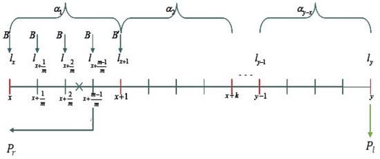
Figure 3. Schematic drawing of the accumulative pension scheme with m-thly payable contributions and a lump sum payment on retirement and with possibility of inheritance. The cross indicates the moment of death.

Since the life table functions in the published mortality tables are given for exact integer ages, actuaries make fractional age assumptions when insurance event occurs at non-integer ages. A fractional age assumption is an interpolation of life table functions between integer age values which are accepted as given. Three fractional age assumptions have been widely used by actuaries: the uniform distribution of death (UDD) assumption, the constant force assumption and the hyperbolic or Balducci assumption (see [5,6]). For Scheme 3, we apply the uniform distribution of death assumption. UDD assumption is equivalent to the linear interpolation of $l_z$:

$$l_{z+t}=(1-t)l_z+t{l}_{z+1}\mathrm{for}\mathrm{integer}z\mathrm{and}t\in [0,1].$$

(7)

Proposition 3.

Consider the pension Scheme 3. Then, under UDD assumption, the balance equation has the form

$$B\sum _{k=0}^{y-x-1}\left(1-{\alpha }_{k+1}\right)\sum _{j=0}^{m-1}{\nu }^{k+\frac{j}{m}}\left({}_k{p}_x-\frac{j}{m}{}_{k|}{q}_x\right)=P_r^{\prime }+P_l{}_{y-x}{p}_x{\nu }^{y-x},$$

(8)

where

$$P_r^{\prime }=\frac{P_r}{l_x}=\frac{B}{m}\sum _{k=1}^{m(y-x)-1}{}_{\lfloor \frac{k-1}{m}\rfloor |}{q}_x\sum _{j=1}^k\left(1-{\alpha }_{\lfloor \frac{j-1}{m}\rfloor +1}\right){\nu }^{\lfloor \frac{j-1}{m}\rfloor +\frac{\left(j-1\right)modm}{m}}$$

(9)

and $\lfloor ·\rfloor$ is the floor function.

In particular, the m-thly payable gross premium B is equal to

$$B=\frac{P_l{}_{y-x}{p}_x{\nu }^{y-x}}{{\displaystyle \sum _{k=0}^{y-x-1}}(1-{\alpha }_{k+1}){\displaystyle \sum _{j=0}^{m-1}}{\nu }^{k+\frac{j}{m}}\left({}_k{p}_x-\frac{j}{m}{}_{k|}{q}_x\right)-P_r^{″}},$$

(10)

where $P_r^{″}=P_r^{\prime }/B$.

Proof of Proposition 3. 

For the convenience of calculation of the balance equation, we give in Table 1 the present values of net contributions (PVNCs) and payments (PVPs) to the inheritors for each period. The last line consists of the present value of the lump sum payments (PVLS).

Table 1. Present values of individual net contributions and payments to the inheritors by period (except the last line). The last line consists of the present value of the lump sum payments.

Age	PVNCs	PVPs
x	$l_{x}B(1-{\alpha }_1){\nu }^0$	0
$x+\frac{1}{m}$	$l_{x+\frac{1}{m}}B(1-{\alpha }_1){\nu }^{\frac{1}{m}}$	$\left(l_x-l_{x+\frac{1}{m}}\right)B(1-{\alpha }_1){(i+1)}^{\frac{1}{m}}{\nu }^{\frac{1}{m}}=$
		$=\left(l_x-l_{x+\frac{1}{m}}\right)B(1-{\alpha }_1){\nu }^0$
$x+\frac{2}{m}$	$l_{x+\frac{2}{m}}B\left(1-{\alpha }_1\right){\nu }^{\frac{2}{m}}$	$\left(l_{x+\frac{1}{m}}-l_{x+\frac{2}{m}}\right)B\left[\left(1-{\alpha }_1\right){(i+1)}^{\frac{1}{m}}+\right.$
		$\left.+\left(1-{\alpha }_1\right){(i+1)}^{\frac{2}{m}}\right]{\nu }^{\frac{2}{m}}=$
		$=\left(l_{x+\frac{1}{m}}-l_{x+\frac{2}{m}}\right)B\left[\left(1-{\alpha }_1\right){\nu }^0+\left(1-{\alpha }_1\right){\nu }^{\frac{1}{m}}\right]$
⋮	⋮	⋮
$x+1$	$l_{x+1}B\left(1-{\alpha }_2\right){\nu }^1$	$\left(l_{x+\frac{m-1}{m}}-l_{x+1}\right)B\left[\left(1-{\alpha }_1\right){(i+1)}^{\frac{1}{m}}+\right.$
		$+\left(1-{\alpha }_1\right){(i+1)}^{\frac{2}{m}}+\dots +$
		$\left.+\left(1-{\alpha }_1\right){(i+1)}^{\frac{m-1}{m}}+\left(1-{\alpha }_1\right){(i+1)}^1\right]{\nu }^1=$
		$=\left(l_{x+\frac{m-1}{m}}-l_{x+1}\right)B\left[\left(1-{\alpha }_1\right){\nu }^0+\left(1-{\alpha }_1\right){\nu }^{\frac{1}{m}}+\right.$
		$\left.+\left(1-{\alpha }_1\right){\nu }^{\frac{2}{m}}+\dots +\left(1-{\alpha }_1\right){\nu }^{\frac{m-1}{m}}\right]$
$x+1+\frac{1}{m}$	$l_{x+1+\frac{1}{m}}B\left(1-{\alpha }_2\right){\nu }^{1+\frac{1}{m}}$	$\left(l_{x+1}-l_{x+1+\frac{1}{m}}\right)B\left[\left(1-{\alpha }_2\right){(i+1)}^{\frac{1}{m}}+\right.$
		$+\left(1-{\alpha }_1\right){(i+1)}^{\frac{2}{m}}+\dots \left(1-{\alpha }_1\right){(i+1)}^{\frac{m-1}{m}}+$
		$+\left.\left(1-{\alpha }_1\right){(i+1)}^1+\left(1-{\alpha }_1\right){\left(i+1\right)}^{1+\frac{1}{m}}\right]{\nu }^{1+\frac{1}{m}}=$
		$=\left(l_{x+1}-l_{x+1+\frac{1}{m}}\right)B\left[\left(1-{\alpha }_2\right){\nu }^1+\right.$
		$+\left(1-{\alpha }_1\right){\nu }^{\frac{m-1}{m}}+\dots +\left(1-{\alpha }_1\right){\nu }^{\frac{2}{m}}+$
		$\left.+\left(1-{\alpha }_1\right){\nu }^{\frac{1}{m}}+\left(1-{\alpha }_1\right){\nu }^0\right]$
⋮	⋮	⋮
$y-1+\frac{1}{m}$	$l_{y-1+\frac{1}{m}}B\left(1-{\alpha }_{y-x}\right){\nu }^{y-x-1+\frac{1}{m}}$	$\left(l_{y-1}-l_{y-1+\frac{1}{m}}\right)B\left[\left(1-{\alpha }_{y-x}\right){(i+1)}^{\frac{1}{m}}+\right.$
		$+\left(1-{\alpha }_{y-x-1}\right){(i+1)}^{\frac{2}{m}}+\dots +$
		$+\left(1-{\alpha }_{y-x-1}\right){(i+1)}^{1+\frac{1}{m}}+$
		$+\dots +\left(1-{\alpha }_1\right){(i+1)}^{y-x-2+\frac{1}{m}}+\dots +$
		$\left.+\dots +\left(1-{\alpha }_1\right){(i+1)}^{y-x-1+\frac{1}{m}}\right]{\nu }^{y-x-1+\frac{1}{m}}=$
		$=\left(l_{y-1}-l_{y-1+\frac{1}{m}}\right)B\left[\left(1-{\alpha }_{y-x}\right){\nu }^{y-x-1}+\right.$
		$\left.\left(1-{\alpha }_{y-x-1}\right){\nu }^{y-x-1-\frac{1}{m}}+\dots +\left(1-{\alpha }_1\right){\nu }^0\right]$
⋮	⋮	⋮
$y-1+\frac{m-1}{m}$	$l_{y-1+\frac{m-1}{m}}B\left(1-{\alpha }_{y-x}\right){\nu }^{y-x-1+\frac{m-1}{m}}$	$\left(l_{y-1+\frac{m-2}{m}}-l_{y-1+\frac{m-1}{m}}\right)B\left[\left(1-{\alpha }_{y-x}\right){(i+1)}^{\frac{1}{m}}+\right.$
		$+\left(1-{\alpha }_{y-x}\right){(i+1)}^{\frac{2}{m}}+\dots +\left(1-{\alpha }_{y-x}\right){(i+1)}^{\frac{m-1}{m}}+$
		$+\dots +\left(1-{\alpha }_1\right){(i+1)}^{y-x-1}+\dots +$
		$+\left.\left(1-{\alpha }_1\right){(i+1)}^{y-x-1+\frac{m-1}{m}}\right]{\nu }^{y-x-1+\frac{m-1}{m}}=$
		$=\left(l_{y-1+\frac{m-2}{m}}-l_{y-1+\frac{m-1}{m}}\right)B\left[\left(1-{\alpha }_{y-x}\right){\nu }^{y-x-1+\frac{2}{m}}+\right.$
		$+\left(1-{\alpha }_{y-x}\right){\nu }^{y-x-1+\frac{1}{m}}+$
		$\left.+\left(1-{\alpha }_{y-x}\right){\nu }^{y-x-1}+\dots +\left(1-{\alpha }_1\right){\nu }^0\right]$
		PVLS
y	0	$P_l{l}_y{\nu }^{y-x}$

Denote respectively by

$$PVNC=\sum PVNCs,PVP=\sum PVPs$$

the present values of all net contributions and payments to the inheritors. Then, the balance equation has the form

$$PVNC=PVP+PVLS.$$

(11)

According to Table 1, the present value of the net contributions is

$$PVNC=l_{x}B(1-{\alpha }_1){\nu }^0+l_{x+\frac{1}{m}}B(1-{\alpha }_1){\nu }^{\frac{1}{m}}+l_{x+\frac{2}{m}}B(1-{\alpha }_1){\nu }^{\frac{2}{m}}+\dots +l_{x+1}B(1-{\alpha }_2){\nu }^1+$$

$$+l_{x+1+\frac{1}{m}}B(1-{\alpha }_2){\nu }^{1+\frac{1}{m}}+\dots +l_{y-1+\frac{1}{m}}B(1-{\alpha }_{y-x}){\nu }^{y-x-1+\frac{1}{m}}+\dots +$$

$$+l_{y-1+\frac{m-1}{m}}B(1-{\alpha }_{y-x}){\nu }^{y-x-1+\frac{m-1}{m}}.$$

(12)

According to Table 1, the present value of the payments is

$$PVP=\left(l_x-l_{x+\frac{1}{m}}\right)B(1-{\alpha }_1){\nu }^0+\left(l_{x+\frac{1}{m}}-l_{x+\frac{2}{m}}\right)B\left[(1-{\alpha }_1){\nu }^0+(1-{\alpha }_1){\nu }^{\frac{1}{m}}\right]+\dots +$$

$$+\left(l_{x+\frac{m-1}{m}}-l_{x+1}\right)B\left[(1-{\alpha }_1){\nu }^0+(1-{\alpha }_1){\nu }^{\frac{1}{m}}+(1-{\alpha }_1){\nu }^{\frac{2}{m}}+\dots +(1-{\alpha }_1){\nu }^{\frac{m-1}{m}}\right]+\dots +$$

$$+\left(l_{y-1}-l_{y-1+\frac{1}{m}}\right)B\left[(1-{\alpha }_{y-x}){\nu }^{y-x-1}+(1-{\alpha }_{y-x-1}){\nu }^{y-x-1-\frac{1}{m}}+\dots +\right.$$

$$+(1-{\alpha }_1){\nu }^0+\dots +\left(l_{y-1+\frac{m-2}{m}}-l_{y-1+\frac{m-1}{m}}\right)B\left[(1-{\alpha }_{y-x}){\nu }^{y-x-1+\frac{2}{m}}+\right.$$

$$\left.+(1-{\alpha }_{y-x}){\nu }^{y-x-1+\frac{1}{m}}+(1-{\alpha }_{y-x}){\nu }^{y-x-1}+\dots +(1-{\alpha }_1){\nu }^0\right].$$

(13)

The present value of the lump sum payments (PVLS) is

$$PVLS=P_l{l}_y{\nu }^{y-x}.$$

(14)

Under the assumption of uniform distribution of deaths, we have (see (7))

$$l_{x+k+\frac{j}{m}}=\left(1-\frac{j}{m}\right)l_{x+k}+\frac{j}{m}{l}_{x+k+1}=l_{x+k}-\frac{j}{m}\left(l_{x+k}-l_{x+k+1}\right),$$

(15)

where x, k are integers and $j/m\in [0,1]$. Hence, $PVNC$ can be rewritten as

$$PVNC=B\left[\left(1-{\alpha }_1\right)\left\{l_x{\nu }^0+\left(l_x-\frac{1}{m}\left(l_x-l_{x+1}\right)\right){\nu }^{\frac{1}{m}}+\left(l_x-\frac{2}{m}\left(l_x-l_{x+1}\right)\right){\nu }^{\frac{2}{m}}+\right.\right.$$

$$\left.+\dots +\left(l_x-\frac{m-1}{m}\left(l_x-l_{x+1}\right)\right){\nu }^{\frac{m-1}{m}}\right\}+$$

$$+\left(1-{\alpha }_2\right)\left\{l_{x+1}{\nu }^1+\left(l_{x+1}-\frac{1}{m}\left(l_{x+1}-l_{x+2}\right)\right){\nu }^{1+\frac{1}{m}}+\dots +\right.$$

$$+\left.\left(l_{x+1}-\frac{m-1}{m}\left(l_{x+1}-l_{x+2}\right)\right){\nu }^{1+\frac{m-1}{m}}\right\}+\dots +\left(1-{\alpha }_{y-x}\right)\left\{l_{y-1}{\nu }^{y-x-1}+\right.$$

$$\left.+\left.\left(l_{y-1}-\frac{1}{m}\left(l_{y-1}-l_y\right)\right){\nu }^{y-x-1+\frac{1}{m}}+\dots +\left(l_{y-1}-\frac{m-1}{m}\left(l_{y-1}-l_y\right)\right){\nu }^{y-x-1+\frac{m-1}{m}}\right\}\right].$$

(16)

Consider now $PVP$. From (15), it follows that

$$l_{x+k+\frac{j}{m}}-l_{x+k+\frac{j+1}{m}}=\frac{1}{m}\left(l_{x+k}-l_{x+k+1}\right),$$

(17)

where x, k are integers and $j/m,(j+1)/m\in [0,1]$. Hence, $PVP$ can be rewritten as

$$PVP=\frac{1}{m}\left(l_x-l_{x+1}\right)B\left(1-{\alpha }_1\right){\nu }^0+\frac{1}{m}\left(l_x-l_{x+1}\right)B\left[\left(1-{\alpha }_1\right){\nu }^0+\left(1-{\alpha }_1\right){\nu }^{\frac{1}{m}}\right]+\dots +$$

$$+\frac{1}{m}\left(l_x-l_{x+1}\right)B\left[\left(1-{\alpha }_1\right){\nu }^0+\left(1-{\alpha }_1\right){\nu }^{\frac{1}{m}}+\left(1-{\alpha }_1\right){\nu }^{\frac{2}{m}}+\dots +\left(1-{\alpha }_1\right){\nu }^{\frac{m-1}{m}}\right]+$$

$$+\dots +\frac{1}{m}\left(l_{y-1}-l_y\right)B\left[\left(1-{\alpha }_{y-x}\right){\nu }^{y-x-1}+\right.$$

$$\left.+\left(1-{\alpha }_{y-x-1}\right){\nu }^{y-x-1-\frac{1}{m}}+\dots +\left(1-{\alpha }_1\right){\nu }^0\right]+$$

$$+\frac{1}{m}\left(l_{y-1}-l_y\right)B\left[\left(1-{\alpha }_{y-x}\right){\nu }^{y-x-1+\frac{2}{m}}+\left(1-{\alpha }_{y-x}\right){\nu }^{y-x-1+\frac{1}{m}}+\right.$$

$$\left.+\left(1-{\alpha }_{y-x}\right){\nu }^{y-x-1}+\dots +\left(1-{\alpha }_1\right){\nu }^0\right].$$

(18)

Multiplying both sides of the balance Equation (11) by $1/l_x$ and taking into account (14), (16) and (18), we obtain

$$\frac{1}{l_x}PVNC=B\left[\left(1-{\alpha }_1\right)\left\{{}_0{p}_x{\nu }^0+\left({}_0{p}_x-\frac{1}{m}{}_{0|}{q}_x\right){\nu }^{\frac{1}{m}}+\left({}_0{p}_x-\frac{2}{m}{}_{0|}{q}_x\right){\nu }^{\frac{2}{m}}+\dots +\right.\right.$$

$$\left.+\left({}_0{p}_x-\frac{m-1}{m}{}_{0|}{q}_x\right){\nu }^{\frac{m-1}{m}}\right\}+\left(1-{\alpha }_2\right)\left\{{}_1{p}_x{\nu }^1+\left({}_1{p}_x-\frac{1}{m}{}_{1|}{q}_x\right){\nu }^{1+\frac{1}{m}}+\dots +\right.$$

$$\left.+\left({}_1{p}_x-\frac{m-1}{m}{}_{1|}{q}_x\right){\nu }^{1+\frac{m-1}{m}}\right\}+\dots +\left(1-{\alpha }_{y-x}\right)\left\{{}_{y-x-1}{p}_x{\nu }^{y-x-1}+\right.$$

$$+\left({}_{y-x-1}{p}_x-\frac{1}{m}{}_{y-x-1|}{q}_x\right){\nu }^{y-x-1+\frac{1}{m}}+\dots +$$

$$\left.\left.+\left({}_{y-x-1}{p}_x-\frac{m-1}{m}{}_{y-x-1|}{q}_x\right){\nu }^{y-x-1+\frac{m-1}{m}}\right\}\right]=$$

$$=B\sum _{k=0}^{y-x-1}\left(1-{\alpha }_{k+1}\right)\sum _{j=0}^{m-1}{\nu }^{k+\frac{j}{m}}\left({}_k{p}_x-\frac{j}{m}{}_{k|}{q}_x\right),$$

(19)

$$\frac{1}{l_x}PVP=\frac{1}{m}{}_{0|}{q}_{x}B\left(1-{\alpha }_1\right){\nu }^0+\frac{1}{m}{}_{0|}{q}_{x}B\left[\left(1-{\alpha }_1\right){\nu }^0+\left(1-{\alpha }_1\right){\nu }^{\frac{1}{m}}\right]+\dots +$$

$$+\frac{1}{m}{}_{0|}{q}_{x}B\left[\left(1-{\alpha }_1\right){\nu }^0+\left(1-{\alpha }_1\right){\nu }^{\frac{1}{m}}+\left(1-{\alpha }_1\right){\nu }^{\frac{2}{m}}+\dots +\right.$$

$$+\left.\left(1-{\alpha }_1\right){\nu }^{\frac{m-1}{m}}\right]+\dots +\frac{1}{m}{}_{y-x-1|}{q}_{x}B\left[\left(1-{\alpha }_{y-x}\right){\nu }^{y-x-1}+\right.$$

$$+\left.\left(1-{\alpha }_{y-x-1}\right){\nu }^{y-x-1-\frac{1}{m}}+\dots +\left(1-{\alpha }_1\right){\nu }^0\right]+\frac{1}{m}{}_{y-x-1|}{q}_{x}B\left[\left(1-{\alpha }_{y-x}\right){\nu }^{y-x-1+\frac{2}{m}}+\right.$$

$$+\left.\left(1-{\alpha }_{y-x}\right){\nu }^{y-x-1+\frac{1}{m}}+\left(1-{\alpha }_{y-x}\right){\nu }^{y-x-1}+\dots +\left(1-{\alpha }_1\right){\nu }^0\right]=$$

$$=\frac{B}{m}\sum _{k=1}^{m(y-x)-1}{}_{\left.\lfloor \frac{k-1}{m}\rfloor \right|}{q}_x\sum _{j=1}^k\left(1-{\alpha }_{\lfloor \frac{j-1}{m}\rfloor +1}\right){\nu }^{\lfloor \frac{j-1}{m}\rfloor +\frac{(j-1)modm}{m}},$$

(20)

$$\frac{1}{l_x}PVLS=P_l{}_{y-x}{p}_x{\nu }^{y-x}.$$

(21)

Relations (19)–(21) prove Proposition 3. □

Proof of Proposition 1. 

Relations (1), (2) can be obtained from Proposition 3 if we set in (8)–(10) $P_r=0$ and $m=1$. □

Proof of Proposition 2. 

Relations (3), (4), (6) can be obtained from Proposition 3 if we set in (8)–(10) $m=1$. □

3. Scheme 4. Cumulative Model of Pension Insurance with Possibility of Inheritance Based on Two Decrement Factors (Mortality and Disability) and with Annual Contributions and a Lump Sum Payment on Retirement

This scheme differs from Scheme 2 (Section 2.2) in that it provides for exit from the pension fund for reasons of death, old-age retirement or disability. A schematic drawing of this pension model is presented in Figure 4.

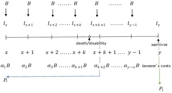
Figure 4. Schematic drawing of the accumulative pension scheme with possibility of inheritance based on two decrement factors and with annual contributions and a lump sum payment on retirement.

For this scheme, some of the actuarial symbols introduced in Section 2 may have another interpretation (the symbols x, y and $d_z$ have the same meaning as in Section 2):

• $l_z$ is the expected number of active insured persons of the pension scheme at age z.
• $P_r$ is the present value of the net contributions refunded to the inheritors/insured if the death/disability occurs before the retirement age. The net contributions are not refunded if the death occurs within the last period of the insurance contract (i.e., within $(y-1,y)$). If the insured person has become disabled within $(y-1,y)$ and reaches the retirement age y, then the pension fund pays him the lump sum at age y.
• $i_z$ is the number of insured persons who leave the pension scheme due to disability between ages z and $z+1$.
• ${}_n{p}_z$ is the probability for an active insured aged z, of being active at age $z+n$. This probability is equal to

  $${}_n{p}_z=\frac{l_{z+n}}{l_z}=1-\frac{{\displaystyle \sum _{j=0}^{n-1}}\left(d_{z+j}+i_{z+j}\right)}{l_z}.$$
  If $z=x$ and $n=y-x$, then according to our assumptions, we have

  $${}_{y-x}{p}_x=\frac{l_y}{l_x}=1-\frac{{\displaystyle \sum _{j=0}^{y-x-2}}\left(d_{x+j}+i_{x+j}\right)+d_{y-1}}{l_x}.$$
• ${}_{n|}{q}_z$ is the probability for an active insured aged z, of being active at age $z+n$ and leaving the pension scheme during the next year (i.e., between ages $z+n$ and $z+n+1$). This probability is equal to

  $${}_{n|}{q}_z=\frac{l_{z+n}-l_{z+n+1}}{l_z}=\frac{d_{z+n}+i_{z+n}}{l_z}.$$

  (22)

Proposition 4.

Consider the pension scheme 4. Then, the balance equation has the form

$$B{\ddot{a}}_{x:\overline{y-x}|}=B\sum _{k=0}^{y-x-1}{\alpha }_{k+1}{\nu }^k{}_k{p}_x+P_l{}_{y-x}{p}_x{\nu }^{y-x}+P_r^{\prime },$$

(23)

where

$$P_r^{\prime }=\frac{P_r}{l_x}=B\sum _{j=1}^{y-x-1}{}_{j-1|}{q}_x\sum _{k=1}^j(1-{\alpha }_k){\nu }^{k-1}.$$

(24)

In particular, the annual gross premium B is equal to

$$B=\frac{P_l{}_{y-x}{p}_x{\nu }^{y-x}}{{\ddot{a}}_{x:\overline{y-x}|}-{\displaystyle \sum _{k=0}^{y-x-1}}{\alpha }_{k+1}{\nu }^k{}_k{p}_x-{\displaystyle \sum _{j=1}^{y-x-1}}{}_{j-1|}{q}_x{\displaystyle \sum _{k=1}^j}(1-{\alpha }_k){\nu }^{k-1}}.$$

(25)

Remark 1.

Although the relations in Propositions 2 and 4 seem to coincide, they have different meanings, since the relations in Proposition 4 contain decrement functions and probabilities. In particular, ${\ddot{a}}_{x:\overline{n}|}$ is the decrement n-year temporary life annuity due.

The proof of this proposition is similar to the proof of Proposition 3 with $m=1$. One can do this with the help of Table 2.

Table 2. Present values of individual net contributions and payments to the inheritors by period (except the last line). The last line consists of the present value of the lump sum payments.

Age	PVNCs	PVPs
x	$l_{x}B\left(1-{\alpha }_1\right){\nu }^0$	0
$x+1$	$l_{x+1}B\left(1-{\alpha }_2\right){\nu }^1$	$\left(d_x+i_x\right)B\left(1-{\alpha }_1\right)\left(i+1\right){\nu }^1=$
		$=\left(d_x+i_x\right)B\left(1-{\alpha }_1\right){\nu }^0$
$x+2$	$l_{x+2}B\left(1-{\alpha }_3\right){\nu }^2$	$\left(d_{x+1}+i_{x+1}\right)B\left[\left(1-{\alpha }_1\right){(i+1)}^2+\right.$
		$+\left.\left(1-{\alpha }_2\right)\left(i+1\right)\right]{\nu }^2=$
		$=\left(d_{x+1}+i_{x+1}\right)B\left[\left(1-{\alpha }_1\right){\nu }^0+\left(1-{\alpha }_2\right){\nu }^1\right]$
⋮	⋮	⋮
$y-1$	$l_{y-1}B\left(1-{\alpha }_{y-x}\right){\nu }^{y-x-1}$	$\left.\left(d_{y-2}+i_{y-2}\right)B\right[\left(1-{\alpha }_1\right){\nu }^0+\left(1-{\alpha }_2\right){\nu }^1+$
		$+\dots +\left(1-{\alpha }_{y-x-1}\right){\nu }^{y-x-2}]$
		PVLS
y	0	$P_l{l}_y{\nu }^{y-x}$

4. Simulation Results and Discussion

A simulation model was developed to analyze the constructed schemes. The annual gross premium was calculated on the base of this simulation model for the schemes with one decrement factor (Section 2.1, Section 2.2 and Section 2.3) and for the scheme with two decrement factors (Section 3). In the calculations, the authors used the male/female mortality table of the Russian Federation for schemes with one decrement factor and the decrement table for the scheme with two factors. A comparative analysis of these four schemes was also carried out.

For calculation purposes, an Excel macro code was written in the VBA programming language (Visual Basic for Applications).

In our calculations, we assumed (we keep the notation of Section 2 and Section 3)

• The retirement age $y=55$ or 60 for females and 60 or 65 for males.
• The age x of the insured person ranges from 18 to y.
• The annual premium loads ${\alpha }_1,\dots ,{\alpha }_{y-x}$ are selected by two rules (deterministic and random rules). Under the deterministic rule, the premium load increases every year by a fixed value, for example by 1%: ${\alpha }_{k+1}={\alpha }_k+0.01$, $k=1,\dots ,y-x-1$ for a given ${\alpha }_1$ (for example ${\alpha }_1=0.05$). Under the random rule, the premium loads are generated by the Excel built-in function RAND. Recall that RAND returns an evenly distributed random real number greater than or equal to 0 and less than 1.
• The effective annual interest rate $i=3\%$, 4% or 5%.
• The lump sum payment may take any non-negative value.

The calculation results show that all the constructed schemes are qualitatively adequate, namely:

• All other things equal, when the accumulation period decreases, the contribution size B increases. The results of some scenarios are shown in Figure 5. In particular, since females reach retirement age earlier than males, the possible accumulation period for females is always shorter. Hence, the contribution size for females is always higher than for males (see Figure 6).
  

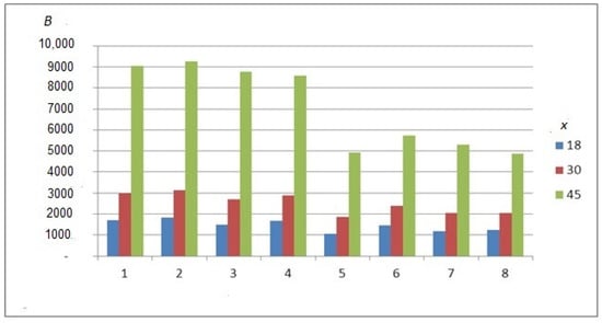  Figure 5. Gross premium size as a function of the accumulation period.
  

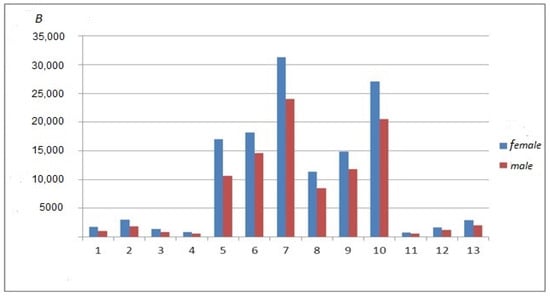  Figure 6. Gross premium size for males and females.
• All other things equal, when the interest rate i increases, the contribution size B decreases. The results of some scenarios are shown in Figure 7.
  

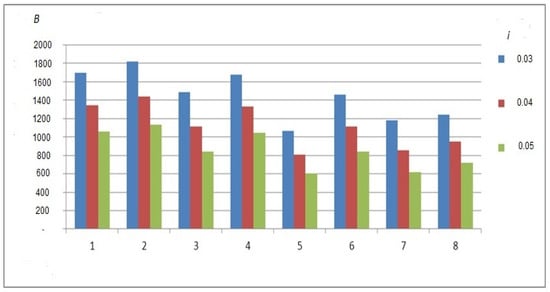  Figure 7. Gross premium size as a function of the interest rate.
• All other things equal, when the lump sum payment $P_l$ decreases the contribution size B also decreases. Namely if we replace $P_l$ by $r{P}_l$ then B is replaced by $rB$ and vice versa. This immediately follows from (2), (6), (10) and (25). The results of some scenarios are shown in Figure 8.
  

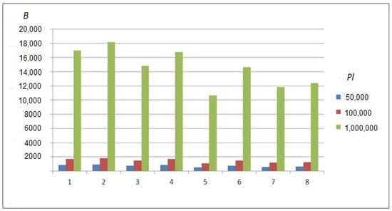  Figure 8. Gross premium size as a function of the lump sum payment.
• For Scheme 3: the lower number of contributions m per year, the higher contribution size B.

Let us now give a comparative analysis of the constructed schemes (see Figure 9).

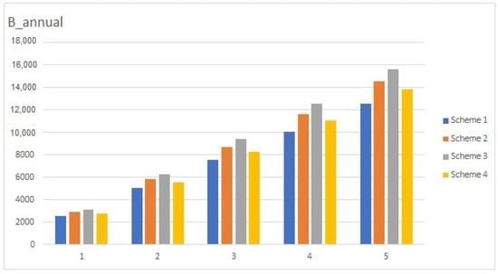
Figure 9. Comparative analysis of Schemes 1–4.

• Consider schemes with one decrement factor (mortality) and annual contributions (Schemes 1 and 2). Then for both genders, all other things equal, the scheme without inheritance (Scheme 1) is the cheapest. This immediately follows from (2) and (6).
• Consider schemes with inheritance and one decrement factor (Schemes 2 and 3). Then for both genders the scheme with at least two contributions per year is more expensive than the scheme with annual contributions (Scheme 2).
• Consider schemes with inheritance and annual contributions (Schemes 2 and 4). Then the scheme with two decrement factors (Scheme 4) is the cheapest.

5. Conclusions

In this work, four accumulative defined contribution pension schemes with a lump sum payment on retirement are proposed. These schemes differ in relation to inheritance and provide various decrement factors. The availability of various schemes allows the insured to choose the most suitable scheme depending on the size of the contribution or the size of the lump sum payment. When choosing a pension scheme, the insured person may have health or family reasons, for example, elderly parents would like to ensure the future of their minor children.

The results of this work are directly related to the Russian draft law of a new system of voluntary retirement savings, called Guaranteed Retirement Plan. In particular, these results are of practical importance for the Pension Fund of the Russian Federation, as well as for private pension funds and pension actuaries in general.

Let us summarize the main results of this work. For each scheme, we use standard methods of actuarial calculations to construct the balance equation and to obtain an expression for the gross premium. A simulation model was developed to analyze the constructed schemes. The gross premium was calculated on the base of this simulation model. A comparative analysis of various schemes was also carried out. According to our calculation, we obtained

• Scheme 1 is the cheapest for the insured person, since it does not provide for the possibility of inheritance and takes into account only one decrement factor (mortality).
• For schemes with inheritance and annual contributions, the scheme with the two decrement factors is the cheapest.
• Consider schemes with one decrement factor (mortality). Then, Scheme 3 with $m>1$ is the most expensive in terms of total annual contribution.

This work can be developed in two directions. It is interesting to consider schemes with a limited inheritance period. This allows one to reduce the size of the gross premium as well as the obligations of the insurer. Since some policyholders may lose jobs and/or do not have funds to pay contributions in full and on time for a certain period, it is interesting to consider schemes that take this into account.

References

- Pension Freedoms and DWP Benefits (Guidance). Published 27 March 2015. Available online: http://gov.uk/government/publications/pension-freedoms-and-dwp-benefits (accessed on 13 November 2020).
- Pension Flexibility: New Options from 6 April 2015 (Guidance). Published 12 February 2015. Available online: https://www.gov.uk/government/publications/pension-flexibility-new-options-from-6-april-2015 (accessed on 13 November 2020).
- Green, N. What Happens to My Pension when I Die? Published 3 September 2020. Available online: https://www.unbiased.co.uk/life/pensions-retirement/pensions-and-inheritance (accessed on 12 November 2020).
- Conner, T. Can I Inherit a Pension? Published 10 October 2019. Available online: https://www.drewberryinsurance.co.uk/knowledge/pensions/can-i-inherit-a-pension (accessed on 12 November 2020).
- Bowers, N.L.; Gerber, H.U.; Hickman, J.C.; Jones, D.A.; Nesbitt, C.J. Actuarial Mathematics; The Society of Actuaries: Schaumburg, IL, USA, 1986; 624p. [Google Scholar]
- Gerber, H.U. Life Lnsurance Mathematics, 3rd ed.; Springer: Berlin/Heidelberg, Germany, 1997; 217p. [Google Scholar]
- Zolotarev, V.M. One-Dimensional Stable Distributions; American Mathematical Society: Providence, RI, USA, 1986. [Google Scholar]
- Uchaikin, V.V.; Zolotarev, V.M. Chance and Stability Stable Distributions and Their Applications; VSP: Utrecht, The Netherlands, 1999; p. 569. [Google Scholar]
- Kalashnikov, V.V. Geometric Sums: Bounds for Rare Events with Applications: Risk Analysis, Reliability, Queueing; Kluwer Academic Publishers: Dordrecht, The Netherlands, 1997. [Google Scholar]
- Kalashnikov, V.V. Two-sided bounds of ruin probabilities. Scand. Actuar. J. 1996, 1, 1–18. [Google Scholar] [CrossRef]
- Kalashnikov, V.V.; Tsitsiashvili, G.S. Asymptotically Correct Bounds of Geometric Convolutions with Subexponential Components; Working Paper No. 151; Lab. of Actuarial Math., Univ. of Copenhagen: Copenhagen, Denmark, 1998. [Google Scholar]
- Korolev, V.; Bening, V.; Shorgin, S. Mathematical Foundations of Risk Theory, 2nd ed.; FIZMATLIT: Moscow, Russia, 2011. [Google Scholar]
- Al-Nator, M.S.; Al-Nator, S.V.; Olenchenko, N.A. Accumulative models of pension insurance. In Materials of Conference on Applied Probability Theory and Theoretical Computer Science; IPI RAN: Moscow, Russia, 2012; pp. 5–7. [Google Scholar]
- Al-Nator, M.S.; Al-Nator, S.V. Accumulative pension scheme with two decrement factors and possibility of inheritance. In Materials of Conference on Information and Telecommunication Technologies and Mathematical Simulation of Hi-Tech Systems; Peoples’ Friendship University of Russia: Moscow, Russia, 2020; pp. 229–232. [Google Scholar]
Publisher’s Note: MDPI stays neutral with regard to jurisdictional claims in published maps and institutional affiliations. |
© 2020 by the authors. Licensee MDPI, Basel, Switzerland. This article is an open access article distributed under the terms and conditions of the Creative Commons Attribution (CC BY) license (http://creativecommons.org/licenses/by/4.0/).