Non-Spiking Laser Controlled by a Delayed Feedback

Abstract

In 1965, Statz et al. (J. Appl. Phys. 30, 1510 (1965)) investigated theoretically and experimentally the conditions under which spiking in the laser output can be completely suppressed by using a delayed optical feedback. In order to explore its effects, they formulate a delay differential equation model within the framework of laser rate equations. From their numerical simulations, they concluded that the feedback is effective in controlling the intensity laser pulses provided the delay is short enough. Ten years later, Krivoshchekov et al. (Sov. J. Quant. Electron. 5394 (1975)) reconsidered the Statz et al. delay differential equation and analyzed the limit of small delays. The stability conditions for arbitrary delays, however, were not determined. In this paper, we revisit Statz et al.’s delay differential equation model by using modern mathematical tools. We determine an asymptotic approximation of both the domains of stable steady states as well as a sub-domain of purely exponential transients.

1. Introduction

One of the unexpected features of early laser systems was the emergence of output pulsations. Even before the first laser has been built, researchers had undertaken studies of instabilities in masers (a maser is a device that produces coherent electromagnetic waves at microwave frequencies through amplification by stimulated emission. The laser works by the same principle as the maser but produces higher frequency coherent radiation at visible wavelengths) and pulsations were actually observed in ruby masers in 1958 [1,2]. The first working laser was a ruby laser made by Maiman in 1960 (the first laser was a solid-state laser: Ruby emitting at $694.3$ nm. Ruby consists of the naturally formed crystal of aluminum oxide (Al${}_2$O${}_3$)) [3]. The complex spiking behavior of ruby lasers [4] was not anticipated and attracted a great deal of theoretical interest (see Figure 1). Similar pulsations have been reported for solid-state, liquid, and gas laser systems.

First derived by Statz and de Mars [6], two rate equations provide a fair description of the laser dynamical response. Computer simulations, however, predicted a train of regular and damped spikes at the output of the laser [7,8,9]. They are called “relaxation oscillations” (ROs). This discrepancy between theory and experiment has to do with the fact that the spiking behavior dies out very slowly. Mechanical and thermal shocks and disturbances present in many lasers, and especially the ruby laser, act to continually re-excite the spiking behavior [10].

It is desirable for some applications to have a smooth output with no or very small amplitude modulation. Non-spiking operation has been achieved in ruby lasers [11,12,13,14] by sampling a portion of the output beam with a photodiode and using the detector signal to control the voltage applied to an electro-optic shutter located inside the resonator. In order to obtain spike suppression, the delay time between the detector and the shutter must be much shorter than the spike width of approximately $0.1$ to 1 $\mathsf{\mu }$s [10].

In 1965, Statz et al. [8] investigated theoretically and experimentally the conditions under which spiking in the laser output can be completely suppressed using a delayed optical feedback. They consider the laser rate equations supplemented by a delayed feedback term. The equations in their original form, as well as their formulation in modern notations, are documented in Appendix A. The same stabilization problem due to a delayed feedback has been later considered by Krivoshchekov et al. [15]. Their rate equations are documented in Appendix B. The delay differential equation (DDE) of Statz et al. [8] has been explored numerically, while the DDE problem of Krivoshchekov et al. [15] has been analyzed for small delays and small feedback gains.

To the best of our knowledge, the publication by Statz et al. [8] is the first one in laser physics, where a DDE problem is clearly formulated. The effect of a delayed feedback on a laser is an important topic in laser physics. In particular, semiconductor lasers (SLs) used in our everyday applications are extremely sensitive to optical feedback. Dynamical instabilities were identified in the early 1970s [16,17] and have been studied since then with various motivations [18,19,20].

The plan of the paper is as follows. Section 2 introduces Statz et al. delay equations and analyzes the stability properties of the non-zero intensity steady state. Section 3 reviews the analysis in [15] based on the short delay limit. Lastly, we discuss the role of the damping rate on the stability conditions.

2. Rate Equations

The basic idea of Statz et al. [8] was to provide additional losses in the laser cavity through a negative delayed feedback. Their objective was to determine the feedback conditions for which damped oscillations are replaced by pure exponential decays. In the dimensionless form, the laser rate equations for the intensity output of the laser I and the population inversion D are given by (see Appendix A for details)

$$\begin{array}{ccc}\hfill \frac{dI}{dt}& =& I\left[-1+D-\delta I(t-\tau )\right],\hfill \end{array}$$

(1)

$$\begin{array}{ccc}\hfill \frac{dD}{dt}& =& \gamma \left[A-D(1+I)\right]\hfill \end{array}$$

(2)

where $A>1$ is the pump parameter and is one control parameter. $\gamma =O\left({10}^{-6}\right)$ is the ratio of the intensity and population time scales. $\delta >0$ and $\tau$ denote the gain and the delay of the feedback, respectively. The values of the parameters used in [8] are documented in Appendix A. We note that $\gamma$ is small. The limit $\gamma \to 0$ is singular because $\gamma$ multiplies the right hand side of Equation (2). We eliminate this singularity by a change of variables described in Appendix A. The new dependent variables x and y represent deviations of I and D with respect to their steady state values $I_s$ and $D_s$[21]$.$ The new time $s=\omega t$ takes into account the basic time scale of the laser damped ROs when the steady state is slightly perturbed. These equations are

$$\begin{array}{ccc}\hfill \frac{dy}{ds}& =& (1+y)\left[x-\eta y(s-\theta )\right],\hfill \end{array}$$

(3)

$$\begin{array}{ccc}\hfill \frac{dx}{ds}& =& -y-\epsilon x(1+I_s(1+y)).\hfill \end{array}$$

(4)

The new parameters $\eta ,$$\theta ,$ and $\epsilon$ are defined in Appendix A. The term multiplying $\epsilon$ in Equation (4) describes the slow damping of the free-running laser intensity oscillations. The delayed term in Equation (1) is a second source of dissipation if the delay $\theta$ is small. Assuming $\eta >>\epsilon ,$ we neglect the term multiplying $\epsilon$ in (4). We obtain

$$\begin{array}{ccc}\hfill \frac{dy}{ds}& =& (1+y)\left[x-\eta y(s-\theta )\right],\hfill \end{array}$$

(5)

$$\begin{array}{ccc}\hfill \frac{dx}{ds}& =& -y.\hfill \end{array}$$

(6)

The non-zero intensity steady state is $(x,y)=(0,0).$ From the linearized equations, we determine the characteristic equation for the growth rate $\lambda .$ It is given by

$${\lambda }^2+\lambda \eta exp(-\lambda \theta )+1=0.$$

(7)

Introducing $\lambda =u+iv$ into Equation (7) and taking the real and imaginary parts provide two equations for u and $v.$ We find

$$\begin{array}{ccc}\hfill u^2-v^2+\eta exp(-u\theta )\left[ucos\left(v\theta \right)+vsin\left(v\theta \right)\right]+1& =& 0,\hfill \end{array}$$

(8)

$$\begin{array}{ccc}\hfill 2uv+\eta exp(-u\theta )\left[-usin\left(v\theta \right)+vcos\left(v\theta \right)\right]& =& 0.\hfill \end{array}$$

(9)

The case of a purely real $\lambda$ corresponds to $v=0.$ From Equation (8), we determine $u=u\left(\eta \right)$ in implicit form as

$$\eta =-\frac{u^2+1}{u}exp\left(u\theta \right)$$

(10)

and since $\eta >0,$$u<0$. The case of complex $\lambda$ has been investigated by solving numerically Equations (8) and (9). Figure 2 represents the real part u as a function of $\eta .$ The full lines correspond to real $\lambda$ for $\theta =0$ (black) and $\theta =0.1$ (red). The broken lines correspond to complex $\lambda$ for $\theta =0$ (black) and $\theta =0.1$ (red). The circles indicate limit points (LPs) where there is a transition between real and complex $\lambda$. If $\theta \ne 0$, the domain of pure exponential decays lies between the two red LPs. They are determined by using (10) and by applying the condition $d\eta /du=0.$ We find that $u=u\left(\theta \right),$ in implicit form, is

$$\theta =\frac{1-u^2}{u(1+u^2)}.$$

(11)

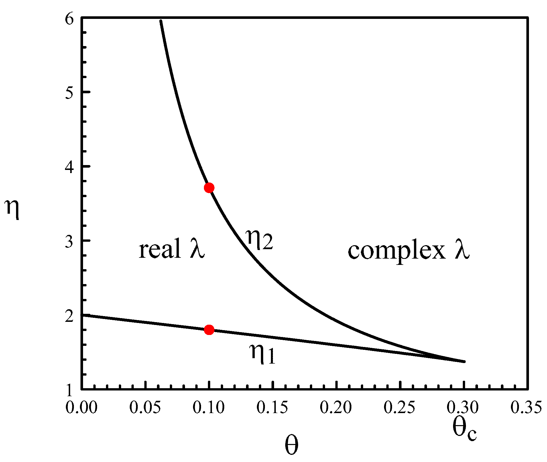
Together with (10), we have a parametric solution for $u\left(\theta \right)$ and $\eta \left(\theta \right).$ We proceed as follows. We progressively decrease u from a low negative value and determine $\theta$ from (11). We then use (10) with $\theta =\theta \left(u\right)$ and determine $\eta .$ The solution $\eta =\eta \left(\theta \right)$ is shown in Figure 3. There is a critical point $\theta ={\theta }_c$ above which no real roots are possible. To find its value, we use (11) and determine $u=u_c$ from the condition $d\theta /du=0.$ We find $u_c=\sqrt{2+\sqrt{5}}.$ We substitute this value into (11) and obtain

$${\theta }_c\simeq 0.3.$$

(12)

If $\theta \to 0,$ we find from (10) and (11), the following approximations for the LPs

$$\begin{array}{ccc}\hfill {\eta }_1& \simeq & 2-2\theta ,\hfill \end{array}$$

(13)

$$\begin{array}{ccc}\hfill {\eta }_2& \simeq & {\theta }^{-1}exp(-1).\hfill \end{array}$$

(14)

The first LP moves to the fixed value ${\eta }_1=2$, while the second LP moves to infinity in the limit of small delays. The later case will be further analyzed in Section 3.

A Hopf bifurcation instability is possible and corresponds to $u=0$. From (8) and (9), we determine the conditions

$$\begin{array}{ccc}\hfill -v^2+\eta vsin\left(v\theta \right)+1& =& 0,\hfill \end{array}$$

(15)

$$\begin{array}{ccc}\hfill \eta vcos\left(v\theta \right)& =& 0.\hfill \end{array}$$

(16)

They admit the solutions

$$\begin{array}{ccc}\hfill \left(1\right)& :& \eta =0,\hfill \end{array}$$

(17)

$$\begin{array}{ccc}\hfill \left(2\right)& :& \eta =\frac{{\theta }_n^2-{\theta }^2}{{\theta }_n\theta }>0,(n=0,2,..),\hfill \end{array}$$

(18)

$$\begin{array}{ccc}\hfill \left(3\right)& :& \eta =\frac{{\theta }^2-{\theta }_n^2}{{\theta }_n\theta }>0(n=1,3,..)\hfill \end{array}$$

(19)

where

$${\theta }_n\equiv \frac{\pi }{2}(1+2n)$$

(20)

and n is detailed in (18) and (19). The dots in Figure 4 are the values considered by Statz et al. [8] in their numerical simulations (listed in

Table A1. Dimensionless parameters and their values.

$\omega =\sqrt{\gamma D_s{I}_s}$	$2.45\times {10}^{-3}$
$\eta =\frac{\delta I_s}{\omega }$	$0.41$, $2.04,$$4.1$
$\epsilon =\frac{\omega }{D_s{I}_s}$	$2.45\times {10}^{-3}$
$\theta =\omega \tau$	$0,$$1.64\times {10}^{-2},8.2\times {10}^{-1},1.7$

). As we can see, five dots are in the domain of unstable steady states. The simulations in [8] were limited in integration time but clearly showed growing oscillations for those values (except for the middle point at $\eta =4)$.

The predictions of the linear stability analysis are verified numerically by simulating Equations (3) and (4). Figure 5a corresponds to $\eta =0$ (no feedback) and exhibits the slowly damped ROs. Figure 5b is for $\eta =1$, which is still part of the domain of decaying oscillations although they are quickly damped. Figure 5c is for $\eta =2.2$, where the decay to the steady state $x=0$ is purely exponential. We note that already for $\eta =1,$ oscillations are strongly damped. This can be explained by considering Equations (3) and (4), and by analyzing the linear stability of $(x,y)=(0,0).$ The characteristic equation for the growth rate $\lambda$ is

$${\lambda }^2+\lambda \left[\eta exp(-\lambda \theta )+\epsilon (1+I_s)\right]+1+\eta \epsilon (1+I_s)exp(-\lambda \theta )=0.$$

(21)

If $\eta =0$, the damping rate of the RO oscillations is given by

$$\mathsf{\Gamma }=\frac{\epsilon }{2}(1+I_s)$$

(22)

as $\epsilon \to 0.$ Assuming $\eta =O\left(\epsilon \right),$ the damping rate is

$$\mathsf{\Gamma }=\frac{1}{2}\left[\epsilon (1+I_s)+\eta cos\left(\theta \right)\right]$$

(23)

in first approximation as $\epsilon \to 0.$ If $cos\left(\theta \right)>0,$ as in Figure 5, $\mathsf{\Gamma }$ increases linearly with $\eta .$

3. Small Delay Limit

Statz et al. [8]’s strategy for eliminating undesired laser oscillations is based on the observation that the roots of the characteristic equation are real and negative if $\eta >2$ in the case of zero delay. In other words, the decay towards the stable steady state is purely exponential if the feedback gain is sufficiently large. Provided that the delay is small, the authors reasonably expected the same transient evolution to the steady state. Krivoshchekov et al. [15] expanded the delayed variable for small $\tau$ as

$$I(t-\tau )=I\left(t\right)-\tau I^{\prime }\left(t\right)+O\left({\tau }^2\right).$$

(24)

They then analyzed the stability of the steady state. Instead of (7), the characteristic equation is

$$(1-\eta \theta ){\lambda }^2+\lambda \eta +1=0$$

(25)

The stability condition is

$$1-\eta \theta >0.$$

(26)

Using

Table A2. Dimensionless parameters and their values.

$\omega =\sqrt{\gamma D_s{I}_s}$	$6.5\times {10}^{-4}$
$\eta =2\frac{{\alpha }^2{I}_s^2}{\omega }$
$\epsilon =\frac{\omega }{D_s{I}_s}$	$2.6\times {10}^{-3}$
$\theta =\omega \tau$
$\theta (max)=\omega \tau (max)$	$9.75\times {10}^{-3}$

in Appendix B, (26) can be rewritten in terms of the original parameters as

$$1-2{\alpha }^2{I}_s^2{\sigma }_0{T}_d^{\prime }>0$$

which is the inequality (5) in [15]. From (25), we determine the conditions for real roots given by

$$\eta >{\eta }_1=2-2\theta +O\left({\theta }^2\right).$$

(27)

The expansion (24) however does not lead to the second LP because ${\eta }_2=O\left({\theta }^{-1}\right)$ is large$.$ The limit where $\eta \sim {\theta }^{-1}$ as $\theta \to 0$ is however interesting because it suggests that a small delay may lead to sustained oscillations provided the negative feedback rate is sufficiently large. A careful analysis of the linearized equations evaluated at the Hopf bifurcation point suggests the following scalings as $\theta \to 0$

$$\overline{\eta }=\theta \eta ,\overline{s}={\theta }^{-1}s,\mathrm{and}\overline{x}={\theta }^{-1}x.$$

(28)

Inserting (28) into Equations (5) and (6) leads to the following equations for $\overline{x}$ and y

$$\begin{array}{ccc}\hfill \frac{dy}{d\overline{s}}& =& (1+y)({\theta }^2\overline{x}-\overline{\eta }y(\overline{s}-1)),\hfill \end{array}$$

(29)

$$\begin{array}{ccc}\hfill \frac{d\overline{x}}{d\overline{s}}& =& -y.\hfill \end{array}$$

(30)

In the limit $\theta \to 0,$ Equation (29) reduces to

$$\frac{dy}{d\overline{s}}=-\overline{\eta }y(\overline{s}-1)(1+y)$$

(31)

which we recognize as Wright equation [22] (or equivalently, the delayed logistic equation, after the change of variable $\overline{y}=1+y$). This specific limit is documented in [23] (p. 117). Oscillations emerge at $\overline{\eta }=\pi /2$ with a period $P=4$ and quickly becomes pulsating as $\overline{\eta }$ is further increased.

4. Discussion

The interest of purely negative real eigenvalues of a DDE is rarely emphasized in the DDE literature essentially devoted to the conditions of oscillatory instabilities. They do, however, play a role in applications, and they strongly depend on the delay.

It is quite remarkable that in 1965, a DDE was analyzed in order to understand how to eliminate undesirable oscillations by using a delayed feedback. Statz et al. [8] were exploring the conditions for purely real eigenvalues as means to obtain exponentially decaying transients. From their experiments and their numerical simulations, they conclude that the delay should be small, and that the feedback gain needs to be sufficiently large. In this paper, we substantiate their findings analytically by determining the conditions

$${\eta }_1\left(\theta \right)<\eta <{\eta }_2\left(\theta \right)\mathrm{and}\theta <{\theta }_c$$

(32)

where ${\eta }_1$ and ${\eta }_2$ admit the approximations (13) and (14) for small delays, respectively, and ${\theta }_c$ is given by (12).

The damping rate $\epsilon$ of the natural laser oscillations is small like ${10}^{-3}$ for the ruby laser, but also for other solid state and semiconductor lasers. In our analysis, we neglect its contribution because the delay term dominates the stability conditions as the feedback rate $\eta$ is increased. However, there are other problems where the damping rate could be moderate to large. Consider, for example, the delayed Duffing equation, which has benefited from recent mathematical interests [24,25,26]. Duffing equation models an elastic pendulum whose spring’s stiffness is nonlinear. Supplemented by a delayed velocity control term, it is given by

$$x^{″}+\epsilon x^{\prime }+x+x^3+c{x}^{\prime }(t-\tau )=0.$$

(33)

The linearized problem leads to the characteristic equation

$${\lambda }^2+\epsilon \lambda +1+c\lambda exp(-\lambda \tau )=0$$

(34)

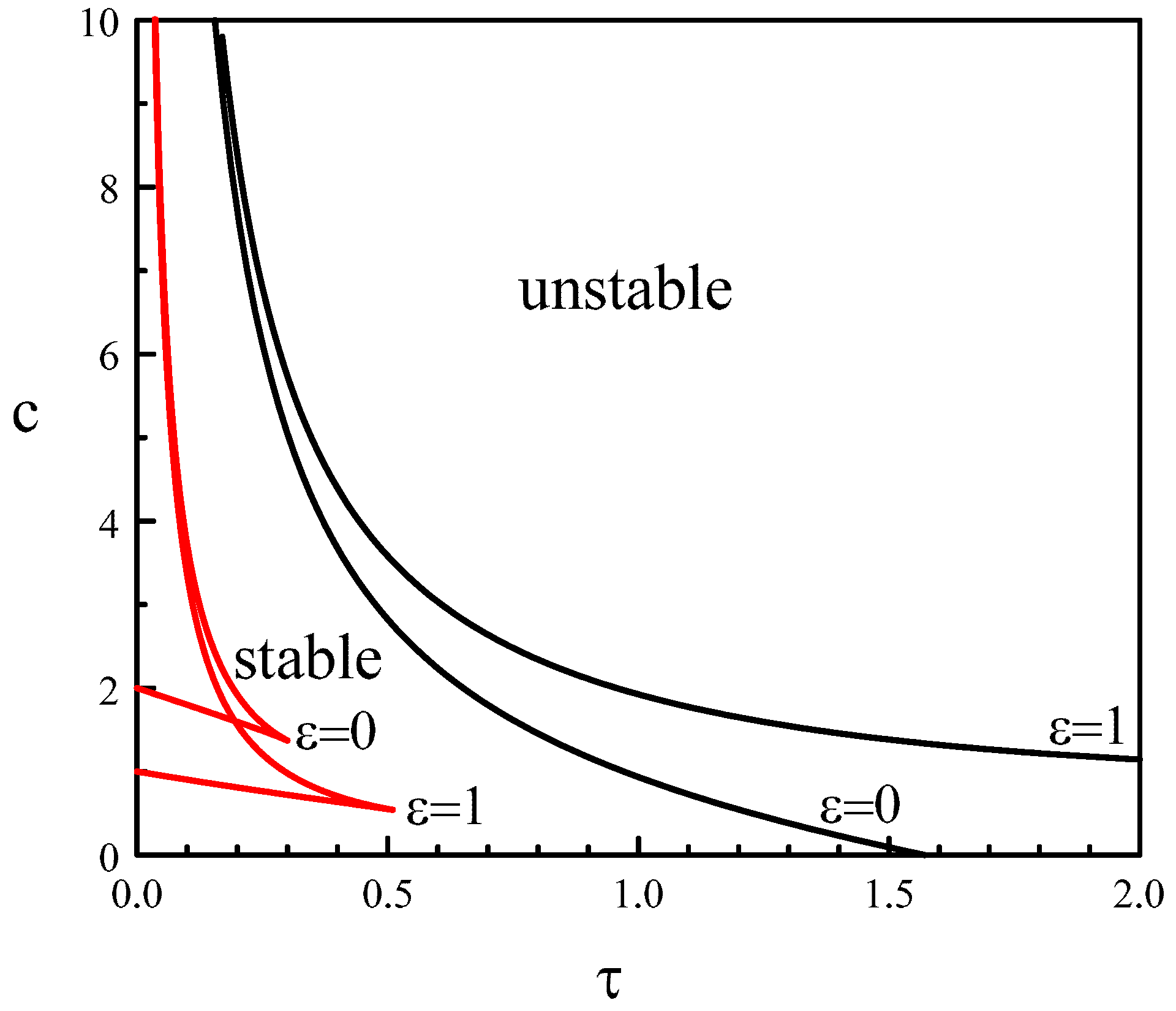
which is Equation (7) supplemented by the $\epsilon \lambda$ term. The analysis of the real and purely imaginary roots of Equation (34) is similar to our previous analysis with $\epsilon =0.$ In Figure 6, we contrast the stability diagrams of $\epsilon =0$ and $\epsilon =1.$ The domain of purely exponential decay increases with $\epsilon$, while the change of stability through a Hopf bifurcation moves to higher delays. This is expected because the damping term contributes to stabilizing the zero solution.