Optimal Exploitation of a General Renewable Natural Resource under State and Delay Constraints

Abstract

In this work, we study an optimization problem arising in the management of a natural resource over an infinite time horizon. The resource is assumed to evolve according to a logistic stochastic differential equation. The manager is allowed to harvest the resource and sell it at a stochastic market price modeled by a geometric Brownian process. We assume that there are delay constraints imposed on the decisions of the manager. More precisely, starting harvesting order and selling order are executed after a delay. By using the dynamic programming approach, we characterize the value function as the unique solution to an original partial differential equation. We complete our study with some numerical illustrations.

1. Introduction

In the recent decades, the management of natural resources has become a major issue. Indeed, for many countries, natural resources ensure regular incomes, allowing for economic growth and development. In particular, the seeking of high short-term profits can lead to an overconsumption of the natural resources and therefore to their exhaustion (see, e.g., [1]). Hence, the question of the sustainability of such natural resources is crucial.

As a consequence, many countries have imposed restrictions on the exploitation of natural resources so as to avoid their depletion. One of the repercussions of these constraints is the non-immediacy of the decisions: the actions of the natural resources managers are executed after some delay. Moreover, the harvests are limited in time, and sometimes, we have a lag constraint between two harvests. The aim of this work is to model these delays and to study their effects on the gain and the behavior of the natural resource managers.

We suppose that the resource manager can act by two type of interventions: starting and stopping the harvesting of the natural resource. We therefore model the strategy by a double sequence ${(d_i,s_i)}_{i\ge 1}$ where $d_i$ and $s_i$ are stopping times representing respectively the time of the i-th decision to start and stop harvesting. Therefore, we assume $s_i\ge d_i$ for $i\ge 1$.

Such a formulation naturally appears in decision-making problems in economics and finance. In many cases, managers face technical and regulatory delays, which may be significant. Thus, these delays need to be taken into account in the way of acting (see for example [2,3]). In our case, we consider the management of a natural resource when we have constraints and lags. We first suppose that there is a minimum time $\delta$ between the end of an action and the beginning of the following one. This constraint can be written on the strategy ${(d_i,s_i)}_{i\ge 1}$ as $d_{i+1}\ge s_i+\delta$ for $i\ge 1$. We also suppose that we have two kind of lags. The first one appears for starting orders: the harvest of the natural resource starts after a given fixed delay ℓ. This delay represents the time needed to access the natural resource. The second kind of lag, denoted by m, corresponds to the time between the end of the harvest and the date when the manager sells the harvest; this lag can be due to the drying, the packaging, the transport, the time to find a counterpart to buy the harvest, etc.

Hence, our modeling takes into account the non-immediacy of both the harvest and its sale. As a result, the corresponding optimal strategies will be more practical and will lead to economic and environmental policies that are more effective than those suggested in the classic literature.

We assume that without any intervention of the manager, the natural resource abundance evolves according to a stochastic logistic diffusion model. Such a logistic dynamics is classic in the modeling of populations’ evolution; see for example [4]. If we denote by $X^{\alpha }$ the controlled resource abundance process and by P its price process, the problem of the manager turns into a maximization of the expected total profit on an infinite horizon of the form:

$$\begin{array}{c}\hfill \mathbb{E}\left[\sum _{i\ge 1}f(d_i,s_i,P_{s_i+m},{\left(X_t^{\alpha }\right)}_{d_i+\ell \le t\le s_i})\right],\end{array}$$

over the strategies $\alpha ={(d_i,s_i)}_{i\ge 1}$ satisfying the previous constraints.

From a mathematical point of view, control problems with delay were studied in [5,6] where there was only one kind of intervention. In our model, we consider two kinds of interventions, which are moreover related by a constraint. In the paper [7], the authors also considered two kinds of interventions. However, there is no constraint linking them, and only one of them is lagged. Furthermore, the state variable (the resource abundance) is a physical quantity. We therefore have the additional state constraint restricting strategies to those in which the remaining abundance is nonnegative.

Control problems under state constraints without delay have been intensely studied in the literature (see for example [8] for the study of optimal portfolio management under liquidity constraints), and the classical approach to deal with such problems is to consider the notion of constrained viscosity solutions introduced in [9,10]. In this work, we adapt these techniques to a state constraints control problem with delay. Using a dynamic programming approach, we characterize the associated value function as the unique solution in the viscosity sense to an original partial differential equation (PDE). The novelty of the PDE lies in the different forms it takes on several regions of the space.

We then test the applicability of our approach by computing numerically the optimal strategies on some examples. Our numerical tests show that the optimal strategies heavily depend on the delay parameters. In particular, the effective optimal strategies are different from the naive optimal strategies, i.e., without delays. This illustrates the contribution of our approach to identifying optimal solutions for the management of natural resources.

The paper is organized as follows. We define the model and formulate our stochastic control problem in Section 2. In Section 3, we derive the partial differential equations associated with the control problem. Then, we characterize the value function as the unique viscosity solution of a Hamilton–Jacobi–Bellman equation. Finally, in Section 4, we compute numerically the value function and the associated optimal policy via an iterative procedure based on a quantization method. We further enrich our studies with numerical illustrations.

2. Problem Formulation

2.1. The Model

Let $\Omega =C({\mathbb{R}}_{+},{\mathbb{R}}^2)$ be the space of continuous functions from ${\mathbb{R}}_{+}$ to ${\mathbb{R}}^2$. We define on $\Omega$ the $\sigma$-algebra $\mathcal{F}$ generated by the coordinate functions $\omega \in \Omega \mapsto {\omega }_t$, for $t\in {\mathbb{R}}_{+}$, and we endow $(\Omega ,\mathcal{F})$ with the Wiener measure $\mathbb{P}$. By an abuse of notation, we still denote by $\mathcal{F}$ the $\mathbb{P}$-completed $\sigma$-algebra. We define on the probability space $(\Omega ,\mathcal{F},\mathbb{P})$ the two $\mathbb{R}$-valued processes B and W by:

$$\begin{array}{ccc}\hfill B_t\left(\omega \right)={\omega }_t^1& \mathrm{and}& W_t\left(\omega \right)={\omega }_t^2,\hfill \end{array}$$

for $t\in {\mathbb{R}}_{+}$ and $\omega ={({\omega }_t^1,{\omega }_t^2)}_{t\ge 0}$. We then denote by $\mathbb{F}={\left({\mathcal{F}}_t\right)}_{t\ge 0}$ the complete filtration generated by $(W,B)$.

We consider a resource that evolves according to the classical logistic stochastic differential equation if there is no harvesting:

$$\begin{array}{ccc}\hfill d{X}_t& =& \eta X_t(\lambda -X_t)dt+\gamma X_{t}d{B}_t,\hfill \end{array}$$

where $\eta$, $\lambda$, and $\gamma$ are three positive constants. The constant $\eta \lambda$ corresponds to the intrinsic rate of population growth, and $1/\lambda$ is the carrying capacity of the environment. A manager can harvest the resource under some conditions. We denote by $\alpha :={(d_i,s_i)}_{i\ge 1}$ a harvesting strategy, which is described as follows.

• $d_i$ is the time at which the manager gives the order to harvest. The harvest starts only at time $d_i+\ell$, with ℓ a positive constant representing the delay.
• $s_i$ is the time when the harvest is stopped.

In the following, we will only consider the set $\mathcal{A}$ of admissible strategies such that ${\left(d_i\right)}_{i\ge 1}$ and ${\left(s_i\right)}_{i\ge 1}$ are two increasing sequences of $\mathbb{F}$-stopping times satisfying:

$$\begin{array}{ccc}\hfill 0& \le s_i-d_i& \le K,\hfill \end{array}$$

(1)

and

$$\begin{array}{ccc}\hfill s_i+\delta & \le & d_{i+1},\hfill \end{array}$$

(2)

for any $i\ge 1$, where $\delta$ and K are positive constants with $\ell <K$.

We assume that in the harvesting time, the manager harvests the quantity $g\left(x\right)$ by the time unit where x is the quantity of the available resource, and g is a function satisfying the following conditions.

(Hg) g is an increasing function from ${\mathbb{R}}_{+}$ to ${\mathbb{R}}_{+}$ such that $g\left(0\right)=0$, and there exist two positive constants $a_{min}$ and $a_{max}$ such that $a_{min}x\le g\left(x\right)\le a_{max}x$ for any $x\in {\mathbb{R}}_{+}$.

Moreover, the manager must pay a cost when he harvests during a period $\Delta t$, and this cost is $f(\Delta t)$ where f is an increasing function from ${\mathbb{R}}_{+}$ to ${\mathbb{R}}_{+}$ such that $f\left(0\right)=0$.

Finally, after any harvest time, the manager sells at time $s_i+m$, with m a positive constant, the harvested resource. We denote by $P^p$ the price of the resource, and we suppose that it evolves according to the following stochastic differential equation:

$$\begin{array}{ccc}\hfill d{P}_t^p& =& P_t^p({\mu }_{t}dt+{\sigma }_{t}d{W}_t),\hfill \\ \hfill P_0^p& =& p,\hfill \end{array}$$

where $\mu$ and $\sigma$ are positive bounded $\mathbb{F}$-adapted processes and p is the price at time 0. We assume that $m<\delta$.

We can sum up all the constraints with the following graph.

The state A corresponds to the state where the manager can decide to start a harvest. The state B corresponds to the harvesting time. The state C corresponds to the moment of sale.

The variable $d_i$ (resp. $s_i$) corresponds to the time when the manager decides to leave the state A (resp. B). The time to go from the state A to the state B is ℓ. This means that the time between the order to harvest and the start of the harvest is ℓ. We cannot stay more than $K-\ell$ in the state B, which means that the harvesting time cannot be more than $K-\ell$. The time to go from the state B to the state C is m. This means that the manager must wait m after the harvest to sell this production. The time to go from the state C to the state A is $\delta -m$, which means that the minimum time between the sale and the next order to harvest is $\delta -m$.

If the manager follows an admissible strategy $\alpha ={(d_i,s_i)}_{i\ge 1}$, then the quantity of available resource $X_t^{x,\alpha }$ at time t evolves with the following stochastic differential equation:

$$\begin{array}{ccc}\hfill d{X}_t^{x,\alpha }& =& \eta X_t^{x,\alpha }(\lambda -X_t^{x,\alpha })dt+\gamma X_t^{x,\alpha }d{B}_t-\sum _{i\ge 1}g\left(X_t^{x,\alpha }\right){\mathbb{1}}_{d_i+\ell \le t\le s_i}dt,\hfill \end{array}$$

(3)

with $X_0^{x,\alpha }=x$.

2.2. The Value Function

The objective of the manager is to optimize the expected profit over an infinite horizon. The associated value function is then given by:

$$\begin{array}{ccc}\hfill V(x,p)& =& \underset{\alpha \in \mathcal{A}}{sup}\mathbb{E}\left[\sum _{i\ge 1}{e}^{-\beta (s_i+m)}(G_i^{\alpha }-C_i^{\alpha })\right],\hfill \end{array}$$

(4)

where $\beta$ is a positive constant corresponding to the discount factor, $G_i^{\alpha }$ and $C_i^{\alpha }$ corresponds to the gain, and the cost for the i-th harvest associated with the strategy $\alpha \in \mathcal{A}$:

$$\begin{array}{ccc}\hfill C_i^{\alpha }& =& f(s_i-d_i-\ell ),\hfill \end{array}$$

(5)

and:

$$\begin{array}{ccc}\hfill G_i^{\alpha }& =& P_{s_i+m}^p{\int }_{d_i+\ell }^{s_i}g\left(X_t^{x,\alpha }\right)dt.\hfill \end{array}$$

(6)

3. PDE Characterization

3.1. Extension of the Value Function

In order to provide an analytic characterization of the value function V defined by (4), we need to extend the definition of this control problem to general initial conditions. Indeed, the delays imposed on the manager make the state process non-Markov. To overcome this issue, we introduce new variables keeping in mind the time spent from the previous decision. More precisely, we consider a gain function $J(x,p,\theta ,\rho ,y,\alpha )$ from $\mathcal{E}:={\mathbb{R}}_{+}\times {\mathbb{R}}_{+}^{*}\times \mathcal{D}\times \mathcal{A}(\Theta )$ to $\mathbb{R}$, with x representing the size of the available resource at the initial time, p the price of the resource, $\theta$ the time from the last decision of the manager (start a harvest or stop a harvest), $\rho$ the time from which the manager has decided to harvest the last time, y the quantity of the harvest until now associated with this harvest, and $\alpha$ the strategy. We introduce some notation to simplify the formulae: $z:=(x,p)$, $\mathcal{Z}:={\mathbb{R}}_{+}\times {\mathbb{R}}_{+}^{*}$ and $\Theta :=(\theta ,\rho ,y)$. We also introduce the following sets:

$$\begin{array}{ccc}\hfill {\mathcal{D}}_0& :=& \{(\theta ,\rho ,y)\in {\mathbb{R}}_{+}^3,y\ge 0,0\le \theta =\rho \le K\},\hfill \\ \hfill {\mathcal{D}}_1& :=& \{(\theta ,\rho ,y)\in {\mathbb{R}}_{+}^3,y\ge 0,0\le \theta <\rho \wedge m\mathrm{and} \rho -K\le \theta \le \rho -\ell \},\hfill \\ \hfill {\mathcal{D}}_2& :=& \{(\theta ,\rho ,y)\in {\mathbb{R}}_{+}^3,y\ge 0,m\le \theta <\rho \mathrm{and} \rho -K\le \theta \le \rho -\ell \},\hfill \end{array}$$

and $\mathcal{D}:={\mathcal{D}}_0\cup {\mathcal{D}}_1\cup {\mathcal{D}}_2$.

The gain function J is given for any state $(z,\Theta )\in \mathcal{Z}\times \mathcal{D}$ and strategy $\alpha \in \mathcal{A}(\Theta )$ by:

$$\begin{array}{ccc}\hfill J(z,\Theta ,\alpha )& :=& \mathbb{E}\left[\sum _{j\ge 1}{e}^{-\beta (s_j+m)}(G_j-C_j)\right],\hfill \end{array}$$

(7)

where $G_1$ and $C_1$ are defined by:

$$\begin{array}{ccc}\hfill G_1& =& \left[y+{\int }_{{(\ell -\theta )}^{+}}^{s_1}g\left(X_s^{x,\alpha }\right)ds\right]P_{s_1+m}^p{\mathbb{1}}_{{\mathcal{D}}_0}+y{P}_{m-\theta }^p{\mathbb{1}}_{{\mathcal{D}}_1},\hfill \\ \hfill C_1& =& f(s_1+\theta -\ell ){\mathbb{1}}_{{\mathcal{D}}_0}+f(\rho -\theta -\ell ){\mathbb{1}}_{{\mathcal{D}}_1}.\hfill \end{array}$$

For any $j\ge 2$, $C_j$ and $G_j$ are defined by (5) and (6).

To define the set of admissible strategies $\mathcal{A}(\Theta )$, we first introduce the set of admissible strategies ${\mathcal{A}}_i(\Theta )$ defined for any $\Theta \in {\mathcal{D}}_i$ with $i\in \{0,1,2\}$:

$$\begin{array}{ccc}\hfill {\mathcal{A}}_0(\Theta )& :=& \{{(d_i,s_i)}_{i\ge 1},\mathrm{where}{d}_1=-\theta ,s_1\mathrm{is}\mathrm{a}\mathrm{stopping}\mathrm{time}\mathrm{valued}\mathrm{in}[{(\ell -\theta )}^{+},K-\theta ]\mathrm{and}\hfill \\ & & {(d_i,s_i)}_{i\ge 2}\in \mathcal{A}\mathrm{with}{d}_2\ge s_1+\delta \},\hfill \end{array}$$

$$\begin{array}{ccc}\hfill {\mathcal{A}}_1(\Theta )& :=& \left\{{(d_i,s_i)}_{i\ge 1},\mathrm{where}(d_1,s_1)=(-\rho ,-\theta )\mathrm{and}{(d_i,s_i)}_{i\ge 2}\in \mathcal{A}\mathrm{with}{d}_2\ge \delta -\theta \right\},\hfill \end{array}$$

$$\begin{array}{ccc}\hfill {\mathcal{A}}_2(\Theta )& :=& \left\{{(d_i,s_i)}_{i\ge 1},\mathrm{where}(d_1,s_1)=(-\rho ,-\theta )\mathrm{and}{(d_i,s_i)}_{i\ge 2}\in \mathcal{A}\mathrm{with}{d}_2\ge {(\delta -\theta )}^{+}\right\}.\hfill \end{array}$$

Finally, we define the set $\mathcal{A}(\Theta )$ by $\mathcal{A}(\Theta )={\mathcal{A}}_i(\Theta )$ when $\Theta \in {\mathcal{D}}_i$ with $i\in \{0,1,2\}$.

We can now define the extended value function v by:

$$\begin{array}{ccc}\hfill v(z,\Theta )& :=& \underset{\alpha \in \mathcal{A}(\Theta )}{sup}\mathbb{E}\left[J(z,\Theta ,\alpha )\right],\hfill \end{array}$$

for any $(z,\Theta )\in \mathcal{Z}\times \mathcal{D}$.

3.2. Dynamic Programming Principle

To characterize the value function v by a PDE, we use the approach by dynamic programming principle. The value function v satisfies the following equalities, which depend on the set in which $\Theta$ lives.

Theorem 1.

For any $z\in \mathcal{Z}$ and $\Theta \in {\mathcal{D}}_0$, we have:

$$\begin{array}{ccc}\hfill v(z,\Theta )& =& \underset{{(\ell -\theta )}^{+}\le s_1\le K-\theta }{sup}\mathbb{E}\left[e^{-\beta s_1}v(X_{s_1}^{x,\alpha },P_{s_1}^p,0,s_1+\theta ,y+{\int }_{{(\ell -\theta )}^{+}}^{s_1}g\left(X_s^{x,\alpha }\right)ds)\right].\hfill \end{array}$$

For any $z\in \mathcal{Z}$ and $\Theta \in {\mathcal{D}}_1$, we have:

$$\begin{array}{ccc}\hfill v(z,\Theta )& =& \mathbb{E}\left[e^{-\beta (m-\theta )}[y{P}_{m-\theta }^p-f(\rho -\theta -\ell )]+e^{-\beta (m-\theta )}v(X_{m-\theta }^{x,\alpha },P_{m-\theta }^p,m,\rho +m-\theta ,0))\right].\hfill \end{array}$$

For any $z\in \mathcal{Z}$ and $\Theta \in {\mathcal{D}}_2$, we have:

$$\begin{array}{ccc}\hfill v(z,\Theta )& =& \underset{{(\delta -\theta )}^{+}\le d_2}{sup}\mathbb{E}\left[e^{-\beta d_2}v(X_{d_2}^{x,\alpha },P_{d_2}^p,0,0,y)\right].\hfill \end{array}$$

The proof of this theorem is postponed to Appendix A, Appendix B and Appendix C.

3.3. Growth Property

We now impose the following assumption on the coefficients:

$$\begin{array}{ccc}\hfill \mu +\eta \lambda -\beta & <& 0.\hfill \end{array}$$

(8)

We then get the following growth property for the value function v. This one will be useful to characterize v as the unique viscosity solution of a PDE system.

Proposition 1.

The value function v satisfies the following growth condition: there exist two positive constants $C_1$ and $C_2$ such that:

$$\begin{array}{ccc}\hfill yp-C_1& \le & v(z,\Theta )\le C_2{(1+|x|}^2+{\left|p\right|}^2),\hfill \end{array}$$

(9)

for any $z=(x,p)\in \mathcal{Z}$ and $\Theta =(\theta ,\rho ,y)\in \mathcal{D}$.

Proof. 

We first prove the left inequality. If $\Theta \in {\mathcal{D}}_0$, we can consider the strategy that consists of stopping the harvest as soon as possible and never harvesting after that, so:

$$\begin{array}{ccc}\hfill v(z,\Theta )& \ge & \mathbb{E}[y{P}_{{(\ell -\theta )}^{+}+m}^p-f\left({(\theta -\ell )}^{+}\right)]\hfill \\ & \ge & yp-f(K-\ell ).\hfill \end{array}$$

If $\Theta \in {\mathcal{D}}_1$, we can consider the strategy that consists of selling the harvest and never harvesting after that, and we get:

$$\begin{array}{ccc}\hfill v(z,\Theta )& \ge & \mathbb{E}[y{P}_{m-\theta }^p-f(\rho -\theta -\ell )]\hfill \\ & \ge & yp-f(K-\ell ).\hfill \end{array}$$

If $\Theta \in {\mathcal{D}}_2$, we can consider the strategy that consists of starting the harvest as soon as possible, stopping this as soon as possible, and never harvesting after that, so:

$$\begin{array}{ccc}\hfill v(z,\Theta )& \ge & \mathbb{E}[y{P}_{{(\delta -\theta )}^{+}+\ell +m}^p-f\left(0\right)]\hfill \\ & \ge & yp-f(K-\ell ).\hfill \end{array}$$

Hence, the left inequality holds with $C_1=f(K-\ell )$.

We now prove the right inequality. For that, we introduce the process ${\overline{X}}^x$ defined by ${\overline{X}}_0^x=x$ and:

$$\begin{array}{ccc}\hfill d{\overline{X}}_t^x& =& \eta {\overline{X}}_t^x(\lambda -{\overline{X}}_t^x)dt+\gamma {\overline{X}}_t^{x}d{B}_t.\hfill \end{array}$$

Using the closed formula of the logistic diffusion (see, e.g., in [11]), we have:

$$\begin{array}{ccc}\hfill {\overline{X}}_t^x& =& \frac{e^{(\eta \lambda -\frac{{\gamma }^2}{2})t+\gamma B_t}}{\frac{1}{x}+\eta {\int }_0^t{e}^{(\eta \lambda -\frac{{\gamma }^2}{2})u+\gamma B_u}du}\hfill \\ & \le & x{e}^{\eta \lambda T}{e}^{-\frac{{\gamma }^2}{2}t+\gamma B_t},\hfill \end{array}$$

which implies the following inequality:

$$\begin{array}{ccc}\hfill \underset{0\le t\le T}{sup}\mathbb{E}\left[{\overline{X}}_t^x\right]& \le & x{e}^{\eta \lambda T}.\hfill \end{array}$$

(10)

We now consider any strategy $\alpha ={(d_i,s_i)}_{i\ge 1}\in \mathcal{A}(\Theta )$. Since the cost function f is positive, we get:

$$\begin{array}{ccc}\hfill J(z,\Theta ,\alpha )& \le & \sum _{i\ge 1}{e}^{-\beta (s_i+m)}\mathbb{E}\left[P_{s_i+m}^p{\int }_{d_i+\ell }^{s_i}g\left({\overline{X}}_s^x\right)ds\right].\hfill \end{array}$$

From Assumption (Hg), we have:

$$\begin{array}{ccc}\hfill J(z,\Theta ,\alpha )& \le & \sum _{i\ge 1}{e}^{-\beta (s_i+m)}\mathbb{E}\left[P_{s_i+m}^p\right]{\int }_{d_i+\ell }^{s_i}{a}_{max}\mathbb{E}\left[{\overline{X}}_s^x\right]ds\hfill \\ & \le & Cp\sum _{i\ge 1}{e}^{(\mu -\beta )s_i}{a}_{max}\underset{0\le t\le s_i}{sup}\mathbb{E}\left[{\overline{X}}_s^x\right].\hfill \end{array}$$

From Inequality (10), we get (C is a generic constant, which can be modified):

$$\begin{array}{ccc}\hfill J(z,\Theta ,\alpha )& \le & Cpx\sum _{i\ge 1}{e}^{(\mu +\eta \lambda -\beta )s_i}.\hfill \end{array}$$

From Inequality (8) and all the constraints about $d_i$ and $s_i$, we know that $s_i\ge Ki+\delta (i-1)+m$ for any $i\in {\mathbb{N}}^{*}$, so we get:

$$\begin{array}{ccc}\hfill J(z,\Theta ,\alpha )& \le & Cpx\sum _{i\ge 1}{e}^{(\mu +\eta \lambda -\beta )(Ki+\delta (i-1)+m)}\hfill \\ & \le & Cpx\sum _{i\ge 1}{e}^{(\mu +\eta \lambda -\beta )(K+\delta )i}\hfill \\ & \le & Cpx,\hfill \end{array}$$

which implies:

$$\begin{array}{ccc}\hfill v(z,\Theta )& \le & Cpx.\hfill \end{array}$$

 □

3.4. Viscosity Properties and Uniqueness

We now consider all the cases to get the PDEs satisfied by the value function v, which is derived from the dynamic programming relation:

• If $\Theta \in {\mathcal{D}}_0$ with $\theta \in [0,\ell )$, that means the manager has given the order to harvest, but this has not yet started, which implies:

  $$\begin{array}{ccc}\hfill \beta v-{\mathcal{L}}^{0}v& =& 0,\hfill \end{array}$$

  (11)

  with ${\mathcal{L}}^0\psi =\eta x(\lambda -x){\partial }_x\psi +\mu p{\partial }_p\psi +\frac{{\left|\gamma x\right|}^2}{2}{\partial }_{xx}\psi +\frac{{\left|\sigma p\right|}^2}{2}{\partial }_{pp}\psi +{\partial }_{\theta }\psi +{\partial }_{\rho }\psi$ for any function $\psi \in C^2(\mathcal{Z}\times \mathcal{D})$.
• If $\Theta \in {\mathcal{D}}_0$ with $\theta \in [\ell ,K)$, that means the manager harvests, and he/she can decide to stop this, which implies:

  $$\begin{array}{ccc}\hfill min(\beta v-{\mathcal{L}}^{1}v,v-{\mathcal{M}}_{1}v)& =& 0,\hfill \end{array}$$

  (12)

  with ${\mathcal{L}}^1\psi =(\eta x(\lambda -x)-g\left(x\right)){\partial }_x\psi +\mu p{\partial }_p\psi +g\left(x\right){\partial }_y\psi +\frac{{\left|\gamma x\right|}^2}{2}{\partial }_{xx}\psi +\frac{{\left|\sigma p\right|}^2}{2}{\partial }_{pp}\psi +{\partial }_{\theta }\psi$$\psi \in C^2(\mathcal{Z}\times \mathcal{D})$, and the operator ${\mathcal{M}}_1$ is defined for any function $v\in C^2(\mathcal{Z}\times {\mathcal{D}}_0)$ by:

  $$\begin{array}{ccc}\hfill {\mathcal{M}}_{1}v(x,p,\theta ,\theta ,y)& =& v(x,p,0,\theta ,y).\hfill \end{array}$$
• If $\Theta \in {\mathcal{D}}_0$ with $\theta =K$, the manager must stop the harvest, so we have:

  $$\begin{array}{ccc}\hfill v(x,p,K,K,y)& =& v(x,p,0,K,y).\hfill \end{array}$$

  (13)
• If $\Theta \in {\mathcal{D}}_1$ with $\theta \in [0,m)$, that means the manager has finished harvesting, but he/she has not yet sold his/her harvest, which implies:

  $$\begin{array}{ccc}\hfill \beta v-{\mathcal{L}}^{0}v& =& 0.\hfill \end{array}$$

  (14)
• If $\Theta \in {\mathcal{D}}_1$ with $\theta =m$, that means the manager sells his/her harvest, which implies:

  $$\begin{array}{ccc}\hfill \underset{\theta \to m^{-}}{lim}v(x,p,\theta ,\rho ,y)& =& yp-f(\rho -m-\ell )+v(x,p,m,\rho ,0).\hfill \end{array}$$

  (15)
• If $\Theta \in {\mathcal{D}}_2$ with $\theta \in [m,\delta )$, then the manager can do nothing, which implies:

  $$\begin{array}{ccc}\hfill \beta v-{\mathcal{L}}^{0}v& =& 0.\hfill \end{array}$$

  (16)
• If $\Theta \in {\mathcal{D}}_2$ with $\theta \ge \delta$, then the manager can decide to start a harvest:

  $$\begin{array}{ccc}\hfill min(\beta v-{\mathcal{L}}^{0}v,v-{\mathcal{M}}_{2}v)& =& 0.\hfill \end{array}$$

  (17)
  The operator ${\mathcal{M}}_2$ is defined for any function $v\in C^2(\mathcal{Z}\times {\mathcal{D}}_2)$ by:

  $$\begin{array}{ccc}\hfill {\mathcal{M}}_{2}v(x,p,\theta ,\rho ,y)& =& v(x,p,0,0,y).\hfill \end{array}$$

As usual, we do not have any regularity property on the value function v. We therefore work with the notion of the viscosity solution.

Definition 1 

(Viscosity solution to (11)–(17)). A locally bounded function w defined on $\mathcal{Z}\times \mathcal{D}$ is a viscosity supersolution (resp. subsolution) if:

• for any $(z,\Theta )\in \mathcal{Z}\times {\mathcal{D}}_0$ and $\phi \in C^2(\mathcal{Z}\times {\mathcal{D}}_0)$ such that:

  $$\begin{array}{ccc}\hfill (w_{*}-\phi )(z,\Theta )& =& \underset{\mathcal{Z}\times {\mathcal{D}}_0}{min}(w_{*}-\phi )\hfill \\ \hfill (resp.(w^{*}-\phi )(z,\Theta )& =& \underset{\mathcal{Z}\times {\mathcal{D}}_0}{max}(w^{*}-\phi ))\hfill \end{array}$$
  we have

  $$\begin{array}{ccc}\hfill \beta \phi (z,\Theta )-{\mathcal{L}}^0\phi (z,\Theta )& \ge & 0if\theta \in [0,l)\hfill \\ \hfill (resp.\beta \phi (z,\Theta )-{\mathcal{L}}^0\phi (z,\Theta )& \le & 0)\hfill \\ \hfill min(\beta \phi (z,\Theta )-{\mathcal{L}}^1\phi (z,\Theta ),w_{*}(z,\Theta )-{\mathcal{M}}_1{w}_{*}(z,\Theta ))& \ge & 0if\theta \in [l,K)\hfill \\ \hfill (resp.min(\beta \phi (z,\Theta )-{\mathcal{L}}^1\phi (z,\Theta ),w^{*}(z,\Theta )-{\mathcal{M}}_1{w}^{*}(z,\Theta ))& \le & 0)\hfill \end{array}$$
• for any $z\in \mathcal{Z}$ and $y\in {\mathbb{R}}_{+}$

  $$\begin{array}{ccc}\hfill w_{*}(x,p,K,K,y)& \ge & w_{*}(x,p,0,K,y)\hfill \\ \hfill (resp.w^{*}(x,p,K,K,y)& \le & w^{*}(x,p,0,K,y))\hfill \end{array}$$
• for any $(z,\Theta )\in \mathcal{Z}\times {\mathcal{D}}_1$ with $\theta \in [0,m)$ and $\phi \in C^2(\mathcal{Z}\times {\mathcal{D}}_1)$ such that:

  $$\begin{array}{ccc}\hfill (w_{*}-\phi )(z,\Theta )& =& \underset{\mathcal{Z}\times {\mathcal{D}}_1}{min}(w_{*}-\phi )\hfill \\ \hfill (resp.(w^{*}-\phi )(z,\Theta )& =& \underset{\mathcal{Z}\times {\mathcal{D}}_1}{max}(w^{*}-\phi ))\hfill \end{array}$$
  we have:

  $$\begin{array}{ccc}\hfill \beta \phi (z,\Theta )-{\mathcal{L}}^0\phi (z,\Theta )& \ge & 0\hfill \\ \hfill (resp.\beta \phi (z,\Theta )-{\mathcal{L}}^0\phi (z,\Theta )& \le & 0)\hfill \end{array}$$
• for any $z\in \mathcal{Z}$, $\rho \in [\ell +m,K+m]$ and $y\in {\mathbb{R}}_{+}$:

  $$\begin{array}{ccc}\hfill w_{*}(x,p,m^{-},\rho ,y)& \ge & yp-f(\rho -\ell )+w_{*}(x,p,m,\rho ,0)\hfill \\ \hfill (resp.w^{*}(x,p,m^{-},\rho ,y)& \le & yp-f(\rho -\ell )+w^{*}(x,p,m,\rho ,0))\hfill \end{array}$$
• for any $(z,\Theta )\in \mathcal{Z}\times {\mathcal{D}}_2$ and $\phi \in C^2(\mathcal{Z}\times {\mathcal{D}}_2)$ such that:

  $$\begin{array}{ccc}\hfill (w_{*}-\phi )(z,\Theta )& =& \underset{\mathcal{Z}\times {\mathcal{D}}_2}{min}(w_{*}-\phi )\hfill \\ \hfill (resp.(w^{*}-\phi )(z,\Theta )& =& \underset{\mathcal{Z}\times {\mathcal{D}}_2}{max}(w^{*}-\phi ))\hfill \end{array}$$
  we have:

  $$\begin{array}{ccc}\hfill \beta \phi (z,\Theta )-{\mathcal{L}}^0\phi (z,\Theta )& \ge & 0if\theta \in [m,\delta )\hfill \\ \hfill (resp.\beta \phi (z,\Theta )-{\mathcal{L}}^0\phi (z,\Theta )& \le & 0)\hfill \\ \hfill min(\beta \phi (z,\Theta )-{\mathcal{L}}^0\phi (z,\Theta ),w_{*}(z,\Theta )-{\mathcal{M}}_2{w}_{*}(z,\Theta ))& \ge & 0if\theta \ge \delta \hfill \\ \hfill (resp.min(\beta \phi (z,\Theta )-{\mathcal{L}}^0\phi (z,\Theta ),w^{*}(z,\Theta )-{\mathcal{M}}_2{w}^{*}(z,\Theta ))& \le & 0)\hfill \end{array}$$

A locally bounded function w defined on $\mathcal{Z}\times \mathcal{D}$ is said to be a viscosity solution to (11)–(17) if it is a supersolution and a subsolution to (11)–(17).

The next result provides the viscosity properties of the value function v.

Theorem 2

(Viscosity characterization). The value function v is the unique viscosity solution to (11)–(17) satisfying the growth condition (9). Moreover, v is continuous on $\mathcal{Z}\times \mathcal{D}$.

The proof of this theorem is postponed in Appendix B.

4. Numerical Results

Unfortunately, we are not able to provide an explicit solution for the HJB Equations (11)–(17). We therefore propose in this section a scheme to approximate the solution v.

4.1. The Discrete Problem

In the following, we introduce the numerical tools to solve the HJB equations related to the value function v. We use a numerical backward scheme based on the optimal quantization mixed with an iterative procedure. The convergence of the solution of the numerical scheme towards the solution of the HJB equation, when the time-space step on a bounded grid goes to zero, can be shown using the standard monotonicity, stability, and consistency arguments. We refer to [12,13] for numerical schemes of the same form.

Each HJB equation of the form $min(\beta v-{\mathcal{L}}^{i}v,v-h_i)=0$, with $i\in \{0,1\}$, will be approximated as follows:

$$\begin{array}{ccc}\hfill v^{n+1}(x,p,\theta ,\rho ,y)& =& max\left\{\mathcal{E}\left[v^{n+1}(X_{\Delta }^i,P_{\Delta },\theta +\Delta ,\rho +\Delta ,Y_{\Delta }^i)\right],h_i^n\right\},\hfill \end{array}$$

where:

$$\begin{array}{ccc}\hfill X_{\Delta }^i& =& x+(\eta x(\lambda -x)-ig\left(x\right))\Delta +\gamma x\sqrt{\Delta }{\xi }_k,\hfill \\ \hfill P_{\Delta }& =& pexp((\mu -{\sigma }^2/2)\Delta +\sigma \sqrt{\Delta }{\xi }_l),\hfill \\ \hfill Y_{\Delta }^i& =& y+ig\left(x\right)\Delta .\hfill \end{array}$$

The constant $\Delta$ represents the time step, and the index n stands for the iteration procedure steps, which are stopped when the error between two consecutive iterations becomes smaller than a given stopping criterion $\epsilon$. The random variables ${\xi }_k$ and ${\xi }_l$ represent the quantization of two independent normally distributed random variables.

Remark 1.

Recall that the optimal quantization technique consists of approximating the expectation $\mathbb{E}\left[f\right(Z\left)\right]$, where Z is a normal distributed variable and f is a given real function, by:

$$\begin{array}{ccc}\hfill \mathcal{E}\left[f\right(\xi \left)\right]& =& \sum _{k\in \xi (\Omega )}f\left(k\right)\mathbb{P}(\xi =k).\hfill \end{array}$$

The distribution of the discrete variable ξ is known for a fixed $N:=card\left(\xi \right(\Omega \left)\right)$, and the approximation is optimal as the $L^2$-error between ξ and Z is of order $1/N$ (see [14]). The optimal grid $\xi (\Omega )$ and the associated weights $\mathbb{P}(\xi =k)$ can be downloaded from the website: http://www.quantize.maths-fi.com/downloads.

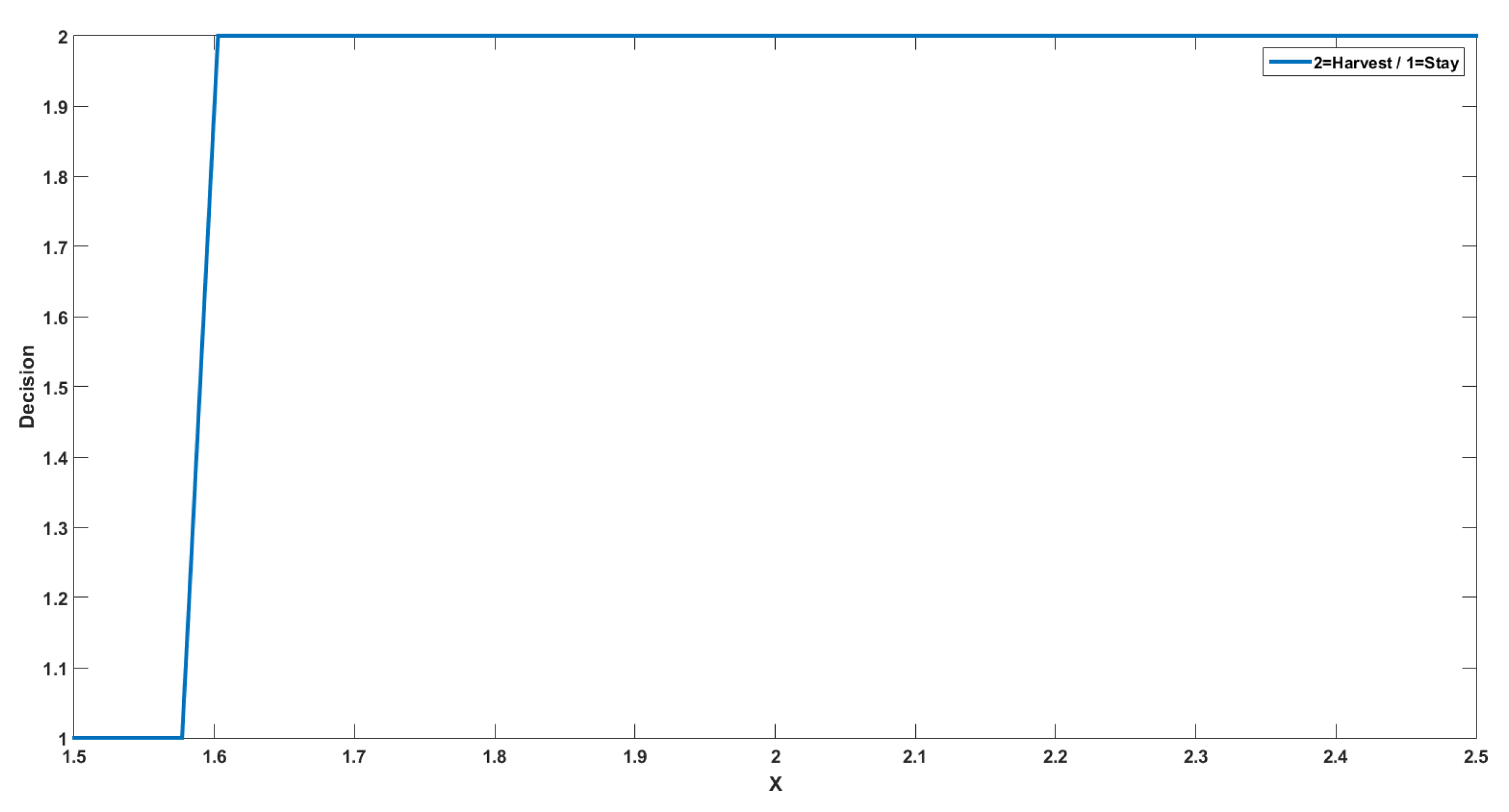
4.2. Numerical Interpretations

The numerical computation is done using the following set of data:

• $\eta =0.1,\lambda =2,\gamma =0.2,\mu =0.2,\sigma =0.1,\beta =0.5$.
• $\delta =K=0.4828,l=m=0.2069$.
• Penalty function: $f\left(x\right)=0.1\times x$.
• Gain function: $g\left(x\right)=x$.

Figure 1. The shape of the value function v for $(x,p,\theta ,\rho ,y)\in {\mathcal{D}}_0$ in the plane of x.

We plot the shape of the value function v for a fixed state $(p,\theta ,\rho ,y)$ in the plane of x s.t. $(x,p,\theta ,\rho ,y)\in {\mathcal{D}}_0$ and $\theta \in [0,\ell )$. We can see that, as expected, v is increasing with respect to x. We can remark about three cases in this figure:

• $x\in [1.5,1.7]$: in this case the, value function is increasing since if we have $1.5\le x<x^{\prime }\le 1.7$ at the initial time, then we will have $X_{\ell -\theta }^x<X_{\ell -\theta }^{x^{\prime }}<2$ a.s., and the bigger is the resource when we harvest, the more we can harvest since the function g is increasing;
• $x\in [1.7,2]$: in this case, the value function is constant since if we have $1.7\le x<x^{\prime }\le 2$ at the initial time then we will have $X_{\ell -\theta }^x=X_{\ell -\theta }^{x^{\prime }}=2$ a.s., so we harvest exactly the same quantity in the two cases;
• $x>2$: in this case, the value function is increasing since if we have $2\le x<x^{\prime }$ at the initial time, then the resource decreases, but we will have $X_{\ell -\theta }^x<X_{\ell -\theta }^{x^{\prime }}$ a.s.

The value function increases with respect to x, which is natural since the greater the resource is, the more we can harvest as the function g is increasing. We can also see that the value function becomes concave after $x=2$, which is due to the resource’s mean-reverting nature. Indeed, if the quantity of the resource is greater than two, because the drift is negative, the resource would necessarily decrease, reducing the harvest. The oscillations observed when x is small are due to the delay ℓ.

Figure 2. The shape of the value function v for $(x,p,\theta ,\rho ,y)\in {\mathcal{D}}_0$ in the plane of x for different values of ℓ.

We plot the shape of the value function v for a fixed state $(p,\theta ,\rho ,y)$ in the plane of x s.t. $(x,p,\theta ,\rho ,y)\in {\mathcal{D}}_0$ and $\theta \in [0,\ell )$ for different values of ℓ. We can see that, when changing the delay time ℓ, the change point of the value function’s monotony is also shifted: $1.6$ for $\ell =0.1379$, $1.7$ for $\ell =0.2069$, and $1.8$ for $\ell =0.2759$. Indeed, as the figure shows, as the delay decreases, the change point of the monotony approaches zero and will likely disappear when there is no delay, leading to a perfect concave function. In fact, wasting time waiting to harvest because of the delay will lead the manager to skip the increasing period of the resource. The manager will start the real harvesting when the population is dropping due to the mean-reverting parameter $\lambda$; thus, the value function will decrease.

Figure 3. The optimal policy for $(x,p,\theta ,\rho ,y)\in {\mathcal{D}}_0$ in the plane of x.

We plot the optimal decision that the manager would make for a fixed state $(p,\theta ,\rho ,y)$ in the plane of x s.t. $(x,p,\theta ,\rho ,y)\in {\mathcal{D}}_0$ and $\theta \in [\ell ,K]$. As we can see, the optimal decision that the manager should make is to start harvesting if the resource x is over a given level; otherwise, he/she should stop and sell the harvest. This is due to the cost f, which penalizes him/her as long as the harvesting is ongoing. In fact, if the population is not large enough, he/she would not be able to cover his/her loss.

Figure 4. The optimal policy for $(x,p,\theta ,\rho ,y)\in {\mathcal{D}}_0$ in the plane of $\theta$.

We plot the optimal decision that the manager would make for four fixed states $(x,p,y)$$(P1,P2,P3,P4)$ in the plane of $\theta$ s.t. $(x,p,\theta ,\rho ,y)\in {\mathcal{D}}_0$. The state $P1$ represents the case where x and y are both low; state $P2$ is for x low and y high, $P3$ for x high and y low, and final state $P4$ for x and y both high. Decision 1 stands for starting the harvest, and Decision 2 stands for stopping it. As we can see, the optimal decision that the manager should make in state $P1$ (resp. $P2$), knowing that he/she has already spent $\theta$ time since the starting decision, is to stop harvesting if $\theta \le {\theta }_0$ (resp. $\theta \le {\theta }_1$) where ${\theta }_0\simeq 0.34$ (resp. ${\theta }_1\simeq 0.38$). We can explain this as follows: on the one hand, in the case where $\theta \le {\theta }_0$ (resp. $\theta \le {\theta }_1$), due to the cost of harvesting and the fact that we are in state $P1$ (resp. $P2$) where the population is low, the manager prefers to immediately stop harvesting and sell the harvest; otherwise, he/she will likely lose money. On the other hand, if $\theta \ge {\theta }_0$ (resp. $\theta \ge {\theta }_1$), i.e., the manager has already given the order to harvest since a given period of time, it is optimal for him/her to harvest for the purpose of covering the cost due to the large time spent harvesting. We can also note that this last window of time is larger for state $P1$ in comparison with the one of state $P2$. Indeed, in state $P2$, the manager has already harvested more than in state $P1$, so he/she can stop harvesting sooner.

Concerning states $P3$ and $P4$, where the population is high, obviously, the optimal decision for the manager is to harvest at all times and stop harvesting when $\theta =K=0.4828$.

Figure 5. The shape of the value function v for $(x,p,\theta ,\rho ,y)\in {\mathcal{D}}_1$ in the plane of p.

We plot the value function v for a fixed state $(x,\theta ,\rho ,y)$ in the plane of p s.t. $(x,p,\theta ,\rho ,y)\in {\mathcal{D}}_1$ and $\theta \in [0,m]$. As expected, v is nondecreasing w.r.t. p. The more expensive the resource is, the more the manager takes benefits.

Figure 6. The optimal policy for $(x,p,\theta ,\rho ,y)\in {\mathcal{D}}_2$ in the plane of x.

We plot the optimal decision that the manager would make for a fixed state $(p,\theta ,\rho ,y)$ in the plane of x s.t. $(x,p,\theta ,\rho ,y)\in {\mathcal{D}}_2$ and $\theta \in [\delta ,{\theta }_{max}]$. As we can see, the optimal decision that the manager should make, knowing that he/she has already sold the harvest, is to start harvesting over a certain level of x under the mean-reverting barrier $\lambda$ so that the population grows enough to cover the harvesting costs and take benefits.

4.3. Conclusions

Our modeling takes into account the non-immediacy of both the harvest and its sale, described by the time delays ℓ and m. The optimum strategies commented on previously illustrate the effect of those delays on the manager’s actions. In the classical literature, many studies suggesting optimal harvesting policies presume that the natural resource is immediately available, which is not the case in general. Consequently, the proposed policies would not be feasible and would lead to a sub-optimal use of the resource, in the best case scenario. The ecological and economic effects may thus be consequential.

For example, a modeling of fisheries that does not involve delays may lead to a harvesting strategy that would likely deplete the fish population, leading to extinction.

In fact, if the population is at a high level at the initial time, it is then likely to decline due to the logistic nature of the dynamics. As a result, if the time required to reach the harvest region is not taken into account, the best approach would be to harvest massively, thus causing a drastic degradation of the fish population.

We may make the same reasoning when it comes to selling the crop. Assume that we are in a position to sell our harvest immediately after harvesting and neglect the time required to return to land. In that case, if the price of fish falls, we would suffer losses, and we would not be able to amortize the costs of fishing.

References

1. Lande, R.; Engen, S.; Sæther, B.-E. Optimal harvesting of fluctuating populations with a risk of extinction. Am. Nat. 1995, 145, 728–745. [Google Scholar] [CrossRef]
2. Alvarez, L.; Keppo, J. The impact of delivery lags on irreversible investment under uncertainty. Eur. J. Oper. Res. 2002, 136, 173–180. [Google Scholar] [CrossRef]
3. Bar-Ilan, A.; Strange, W. Investment lags. Am. Econ. Rev. 1996, 8, 610–622. [Google Scholar]
4. Alvarez, L.; Shepp, L. Optimal harvesting of stochastically fluctuating populations. J. Math. Biol. 1998, 37, 155–177. [Google Scholar] [CrossRef]
5. Bruder, B.; Pham, H. Impulse control problem on finite horizon with execution delay. Stoch. Process. Appl. 2009, 119, 1436–1469. [Google Scholar] [CrossRef] [Green Version]
6. Oksendal, B.; Sulem, A. Optimal Stochastic Impulse Control with Delayed Reaction. Appl. Math. Optim. 2008, 58, 253–298. [Google Scholar] [CrossRef] [Green Version]
7. Kharroubi, I.; Lim, T.; Vath, V.L. Optimal Exploitation of a Resource with Stochastic Population Dynamics and Delayed Renewal. J. Math. Anal. Appl. 2019, 477, 627–656. [Google Scholar] [CrossRef] [Green Version]
8. Mnif, M.; Pham, H. A model of optimal portfolio selection under liquidity risk and price impact. Financ. Stochastics 2007, 11, 51–90. [Google Scholar]
9. Soner, H.M. Optimal Control with State-Space Constraints I. SIAM J. Control. Optim. 1986, 24, 552–561. [Google Scholar] [CrossRef]
10. Soner, H.M. Optimal Control with State-Space Constraints II. SIAM J. Control. Optim. 1986, 24, 1110–1122. [Google Scholar] [CrossRef]
11. Skiadas, C.H. Exact Solutions of Stochastic Differential Equations: Gompertz, Generalized Logistic and Revised Exponential. Methodol. Comput. Appl. Probab. 2010, 12, 261–270. [Google Scholar] [CrossRef]
12. Gaïgi, M.; Vath, V.L.; Mnif, M.; Toum, S. Numerical Approximation for a Portfolio Optimization Problem Under Liquidity Risk and Costs. Appl. Math. Optim. 2016, 74, 163–195. [Google Scholar] [CrossRef]
13. Guilbaud, F.; Mnif, M.; Pham, H. Numerical methods for an optimal order execution problem. J. Comput. Financ. 2013, 16, 3–45. [Google Scholar] [CrossRef] [Green Version]
14. Pagès, G.; Pham, H.; Printems, J. Optimal quantization methods and applications to numerical problems in finance. In Handbook on Numerical Methods in Finance; Rachev, S., Ed.; Birkhäuser: Boston, MA, USA, 2004; pp. 253–298. [Google Scholar]
15. Bouchard, B.; Touzi, N. Weak dynamic programming principle for viscosity solutions. SIAM J. Control. Optim. 2011, 49, 948–962. [Google Scholar] [CrossRef] [Green Version]
16. Dellacherie, C.; Meyer, P.A. Probabilités et Potentiel, I–IV; Hermann: Paris, France, 1975. [Google Scholar]
Figure 1. The shape of the value function v sliced in the plane of x.
Mathematics 08 02053 g001
Figure 2. The shape of the value function v sliced in the plane of x for different values of .
Mathematics 08 02053 g002
Figure 3. The optimal policy for ( x , p , θ [ , K ] , ρ , y ) D 0 in the plane of x.
Mathematics 08 02053 g003
Figure 4. The optimal policy for ( x , p , θ , ρ , y ) D 0 in the plane of θ .
Mathematics 08 02053 g004
Figure 5. The value function v for ( x , p , θ [ 0 , m ] , ρ , y ) D 1 in the plane of p.
Mathematics 08 02053 g005
Figure 6. The optimal policy for ( x , p , θ [ δ , θ m a x ] , ρ , y ) D 2 in the plane of x.
Mathematics 08 02053 g006
Publisher’s Note: MDPI stays neutral with regard to jurisdictional claims in published maps and institutional affiliations.