An Efficient Framework for Adequacy Evaluation through Extraction of Rare Load Curtailment Events in Composite Power Systems

Abstract

With the growing robustness of modern power systems, the occurrence of load curtailment events is becoming lower. Hence, the simulation of these events constitutes a challenge in adequacy indices assessment. Due to the rarity of the load curtailment events, the standard Monte Carlo simulation (MCS) estimator of adequacy indices is not practical. Therefore, a framework based on the enhanced cross-entropy-based importance sampling (ECE-IS) method is introduced in this paper for computing the adequacy indices. The framework comprises two stages. Using the proposed ECE-IS method, the first stage’s purpose is to identify the samples or states of the nodal generation and load that are greatly significant to the adequacy indices estimators. In the second stage, the density of the input variables’ conditional on the load curtailment domain obtained by the first stage are used to compute the nodal and system adequacy indices. The performance of the ECE-IS method is verified through a comparison with the standard MCS method and the recent techniques of rare events simulation in literature. The results confirm that the proposed method develops an accurate estimation for the nodal and system adequacy indices (loss of load probability (LOLP), expected power not supplied (EPNS)) with appropriate convergence value and low computation time.

1. Introduction

Power system reliability evaluation plays a crucial role in the decision-making process of power system development planning. The reliability evaluation process invariably involves consideration of adequacy and security concepts [1,2]. Security is explained as “the measure of how an electric power system can withstand sudden disturbances such as electric short circuits or unanticipated loss of system components”. While adequacy is determined as ”a measure of the ability of a bulk power system to supply the aggregate electric power and energy requirements of the customers within component ratings and voltage limits, taking into account scheduled and unscheduled outages of system components and the operating constraints imposed by operations”. Technically, there is a strong relationship between both concepts, but they are quite different from the economic aspects [3]. This paper mainly concentrates on the adequacy evaluation problem. As a rule, three main functional zones of a power system are highlighted in the part of reliability related to adequacy [1]. HL1 is associated with the total system generation. HL2, in addition to generation facilities, includes transmission facilities. HL3 considers a full power system structure up to individual consumer points. The hierarchical levels mentioned above require power system models of different levels of detail. The adequacy evaluation problem is here considered for HL2.

In power system adequacy analysis, the goal is to assess the effects of uncertain input variables (generations–loads) on the adequacy of a power system. The main indices of the adequacy of power systems are the probability and mathematical expectation of a power shortage (load curtailment) [4]. In practice, a widely used method for the adequacy indices calculation is the Monte Carlo simulation (MCS) because of its advantages [5]. It can handle high-dimensional problems. In addition, the MCS converges, regardless of the complexity of the power system model. Another important aspect is its highly distributable aspect, which allows the calls to the model to be run in parallel. However, the MCS method relies on sampling over the entire input space, no matter where the load curtailment domain is. After that, power flow analysis is needed for each state. Depending on this analysis, corrective actions such as load curtailment and generating unit reschedule are applied in the case of power shortage. The implementation of corrective actions is made through optimization algorithm. The objective of optimization problem is to minimize the total amount of load curtailment constrained to the operating limits of generating units and transmission circuits, and to the power flow equations. As there are several procedures in the evaluation of a state, the computation burden could be very heavy. Moreover, since the modern power systems are now characterized by the rare occurrence of the load curtailment events, the MCS method requires a great number of samples before appropriate load curtailment events are carried out, and so high computation time is needed to reach proper convergence criterion on the estimation of load curtailment probability. Such a computational burden is often unaffordable in practice due to the long runtime of a state evaluation for a power system model. Hence, there are two research tracks for the purpose of overcoming the MCS computational burden. A first research track is to develop high performance programming paradigms [6,7,8,9,10,11,12,13,14,15,16,17,18,19,20] for the purpose of reducing the computation time of state evaluation. A second track could be to derive more efficient sampling techniques [21,22,23,24,25,26,27,28,29,30,31,32,33,34,35,36] for reducing the number of the states needed to be evaluated through concentrating the sampling effort in the regions of interest. This significantly reduces the number of calls to the power system model.

Parallel computing (PAC) [6,7,8], object-oriented programming (OOP) [9], and agent-based technology (ABT) [10,11] are examples of the programming paradigms that can be used to reduce the MCS computational burden. However, the relationship between the number of computing resources and the computational time is close to a linear function [7]. Thus, the hardware could still be expensive. In order to overcome this shortcoming, advanced techniques-based MCS methods have been developed such as pattern classification techniques [12,13,20,21,22] and metamodels or surrogate models [23,24,25,26] to make an equivalent model for the computer code to fasten the computations. Pattern classification techniques are utilized to categorize states (load curtailment or not) of a power system. Some models of these techniques are artificial immune recognition systems [13], artificial neural network [12], least squares support vector machine [20], and deep-learning and multi-label classification methods [21,22]. However, the computational accuracy and flexibility of the model relies on size of training samples. In the structural safety analysis, various types of surrogate models [23,24,25,26] were proposed to change the limit-state functions, which expresses the performance of a system, by an equivalent metamodel-based approximation. These techniques have shown a significant reduction in the computational burden of the MCS method. However, reliability results depend on the accuracy of the surrogate model. Therefore, the accuracy of the surrogate model needs to be ensured to avoid adding uncertainty to the already existing input uncertainty. The main disadvantage to this technique is that there is a difficulty in measuring the impact of the modeling errors on reliability results. Compared with the abovementioned methods, sampling-based methods have the advantages of being insensitive to the complexity of limit-state functions, avoiding errors from approximations of the limit-state function, and being straightforward to apply. Thus, more efficient sampling techniques for overcoming the MCS computation burden are adopted in this paper.

In the context of reducing the number of the states that need to be evaluated, variance reduction techniques enable us to extract the set of states, which make a significant contribution to the evaluation of adequacy indices. Since the variance of the MCS estimate is inversely proportional to the failure probability [5], the variance reduction methods [21,22,23,24,25,26,27,28,29,30,31,32,33,34,35,36] have been developed for reducing the variance of the MCS estimate through generating samples exploring the rare load curtailment events and so shortening the computation time of obtaining an accurate estimate of the adequacy indices. The name of variance reduction techniques gathers various techniques, such as subset sampling [16], importance sampling [17,18,19], control variates [27], antithetic variates [28], stratified sampling [29], line sampling [30,31], and directional sampling [32]. For the sake of conciseness, subset simulation (SS) and importance sampling (IS) are reviewed in this paper, as they are the most substantial variance reduction approaches applied in adequacy studies. SS is based on splitting the failure domain into a series of partial failure domains. This facilitates describing the probability of failure event as a product of conditional probabilities of the partial failure events. The main advantages of SS are its capability to handle complex limit-state functions (e.g., nonlinear, with possibly multiple failure regions). On the other hand, SS have some drawbacks. Firstly, the variance estimator is not directly calculated by an analytical formula as MCS and IS techniques but must be evaluated by repetition. Secondly, even if SS provides a variance reduction compared to MCS, the number of samples needed to achieve convergence is larger than that needed with other IS techniques [16]. The IS techniques propose an alternate sampling density, called the ISD, which is the density of the input variables conditional on the failure domain. The optimal selection of the ISD can result in zero variance of the estimate of failure probability. However, in practice, sampling from the theoretically optimal ISD is not handy, because it needs knowing the failure probability and failure domain in advance. To overcome this problem, the cross-entropy [33,34] and sequential importance sampling (SIS) [35,36] techniques were applied to approximate the optimal ISD in a sequential manner.

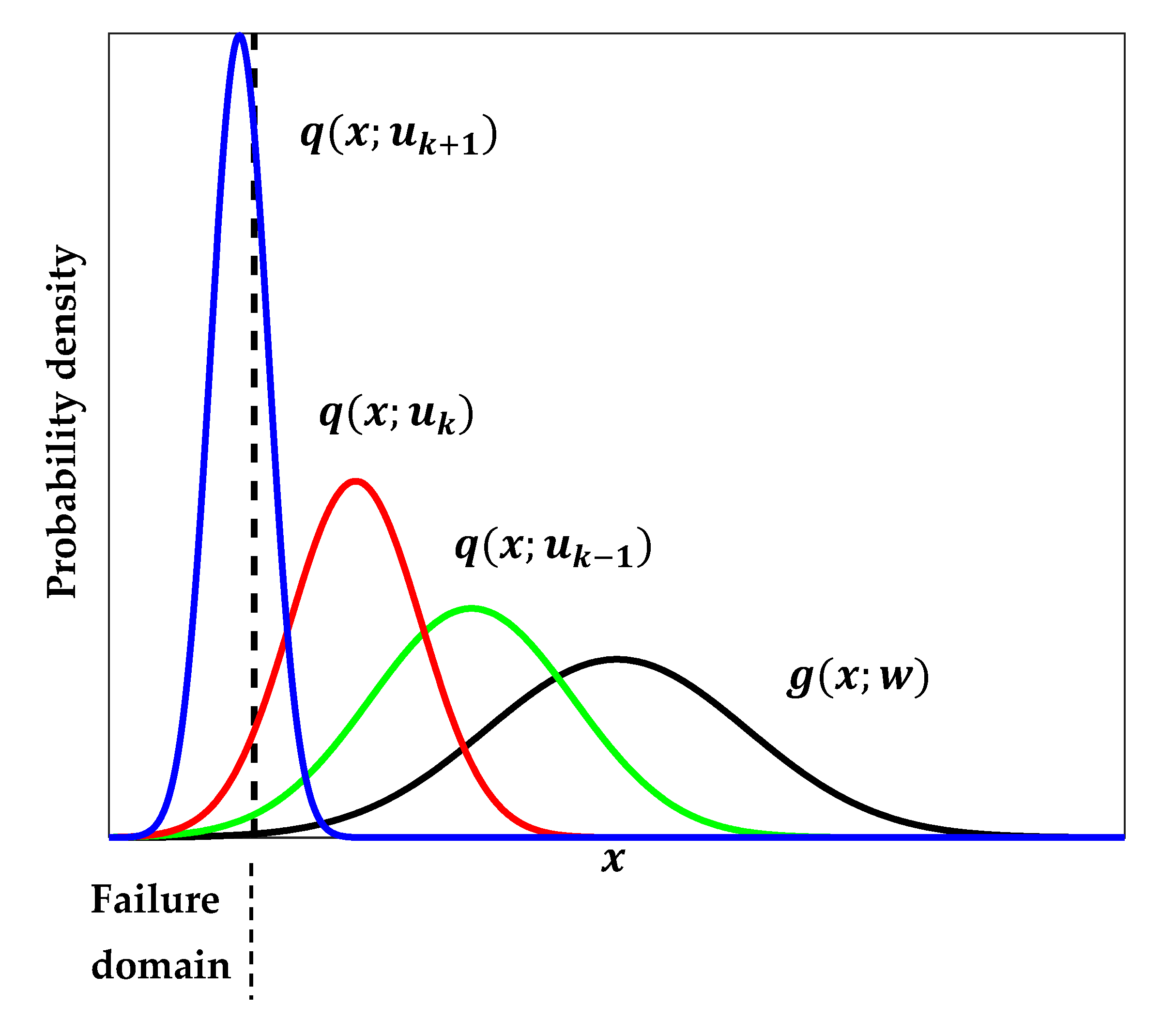
The CE method determines the ISD iteratively through defining a sequence of more frequent events (intermediate failure events) in several probability spaces that gradually reach the target theoretical ISD (small failure event). The densities of intermediate failure events are chosen as parametric family of densities. Typically, the densities are chosen as the same family as the density of the input random variables, and the initial intermediate sampling density is chosen as the original density of the random variables. For each intermediate failure event $k$, the CE method identifies the parameter of a chosen density model through minimizing KL divergence between the optimal ISD of $k$-th intermediate failure event and the chosen probability density. The optimal ISD of $k$-th intermediate failure event is defined based on the intermediate failure threshold (${\zeta }_k\ge 0$), which is estimated such that a fraction ($\theta \in \left[0.01, 0.1\right]$) of the limit-state function values of the samples from the fitted parametric density obtained at the previous sampling step are beyond this threshold ${\zeta }_k$. Starting from an initial sampling density, the density parameter updating is executed until the threshold ${\zeta }_k$ becomes beyond zero (i.e., at least $\theta$ of the limit-state function values of the samples fall in the actual failure domain). In this case, the target optimal ISD is approximated well enough by the current parametric density. The advantage of the CE-IS approach is related to the fact that analytical updating formulas can be derived for density parameters when dealing with probability densities belonging to the natural exponential family. Another advantage concerns the fact that, similarly to the standard MCS, the estimation error is directly controlled using the estimator of the variance [34]. However, the major difficulty is to construct efficient intermediate densities used in the adaptive sampling process to approach the target optimal ISD.

This paper presents an improved version of the CE-IS by incorporating two enhancements. The first one is developing a new updating scheme for the parameter of the intermediate density. In the proposed method, the indicator function of the intermediate failure events is defined by a smooth approximation function instead of using step function as the traditional CE-IS method. This allows exploiting all the samples from intermediate sampling levels in the density parameter updating, contrary to the traditional CE-IS method, which uses a small portion of the samples. In addition, a smooth shifting for the optimal ISD of intermediate failure events towards the target optimal ISD of the small failure event is achieved. This effective use of the intermediate samples leads to better estimate of the density parameter and hence to a smaller sampling error in the corresponding probability estimate. Secondly, exploiting as stopping criterion the coefficient of variation of the weights according to the smooth approximation of the optimal ISD of intermediate failure events with regard to the target optimal ISD improves the robustness of the method convergence. These modifications contribute to obtaining the accurate optimal ISD of nodal generations and loads, and so, the nodal and system adequacy indices are computed accurately. We compare the performance of the proposed method to the traditional CE-IS and recently proposed techniques in literature such as sequential importance sampling and subset simulation. The paper is structured as follows. After a brief introduction, Section 2 illustrates the principles of adequacy assessment in power systems. Moreover, the mathematical objective function and constraints of the optimal power flow (OPF) algorithm are defined. Section 3 describes the framework of adequacy indices evaluation based on the proposed ECE-IS method. In addition, the mathematical description of the ECE-IS is presented. Section 4 depicts the case study and numerical results. The results discussion is explained in Section 5. Section 6 outlines the main findings.

2. Principles of Adequacy Evaluation in Power Systems

For adequacy evaluation purposes, a bulk power system model is normally represented by a group of areas or market nodes connected by transmission lines. Then, the uncertainties of total available generation capacity and total required load are depicted for each area or node. The available capacity of generators in each node can be defined by a binomial distribution. Figure 1 shows the binomial PDF for the failure of $m$ generators in a power plant including $y$ generators with the same probability of failure $(q=5\%$). The probability of failure is calculated using Equation (1).

$${\mathbb{P}}_F^m=C_y^m{q}^m{\left(1-q\right)}^{y-m}$$

(1)

For a large number of generators, according to the de Moivre–Laplace theorem, the binomial distribution could be approximated by a Gaussian one. Such an approach is accepted in this paper. The Gaussian distribution is also used for describing the aggregated load connected to each node. In order to calculate realistic adequacy indices of each node, it is necessary to take into account both load curtailment strategy and physical constraints [37,38]. For each sample within the simulation method, a power flow model must be solved to detect the state of the transmission system. If there are transmission lines outside their loading limits, an OPF algorithm is executed to apply corrective actions (e.g., generation rescheduling and/or load curtailment) by solving an optimization problem. The objective of optimization problem is to minimize the total amount of load curtailment constrained to the operating limits of generating units and transmission circuits, and to the power flow equations. As there are several procedures in the evaluation of a state, a linear representation for the power flow equations is often adopted in HL2 adequacy studies to significantly decrease the computational effort [39]. This representation cannot analyze the impact of bus voltages and reactive power on the system adequacy. This simplification is acceptable, since the adequacy studies mainly deal with long term power system analysis [16]. Hence, a DC-power-flow-based optimization method is used because it is simpler (being linear model) and faster in computation compared with AC power flow.

2.1. Objective Function

A load curtailment sharing philosophy is considered in this work. Unserved demand is shared across all the nodes of a power system. Using weight factors in the objective function, a priority order policy is employed for nodes [18]. The objective function is presented in a quadratic form:

$$min\left({\displaystyle \sum }_{d=1}^n{c}_d{L}_{curt.d}^2\right)$$

(2)

In addition to the objective function, the power system physical constraints are of paramount importance and will strongly affect resulting adequacy indices.

2.2. Constraints

The main aim of adequacy evaluation is to calculate adequacy indices of a power system, while not paying special attention to voltages drops, congestions, and frequency problems of the grid [2]. The nodal power balance constraint can be written in the next form:

$$u_d+G_d+L_{curt.d}-L_d=0,d=1,\dots n$$

(3)

In addition to (3), a system power balance equation is used:

$$u_{\Sigma }+{\pi }_{\Sigma }=0$$

(4)

The power flows vector is calculated using a simplified form of DC power flows equations:

$$\begin{gathered} PF=-\left[B_{br}\right]M^t{B}^{-1}u, \\ PF=-Cu, C=\left[B_{br}\right]M^t{B}^{-1} \end{gathered}$$

(5)

Power losses for each Monte Carlo simulation sample are calculated based on the assumption that all nodal voltages are equal to the nominal ones.

$${\pi }_{\Sigma }={\displaystyle \sum }_{l=1}^{NL}\frac{R_l}{V^2}P{F}_l^2$$

(6)

Power flows through transmission lines are limited by maximum transmission line capacities:

$$-P{F}_{j,d}^{max}\le P{F}_{d,j}\le P{F}_{d,j}^{max}$$

(7)

The generation and curtailed load in each node are restricted by supply and demand bid limits:

$$0\le G_d\le G_d^{av},$$

(8)

$$0\le L_{curt,d}\le L_d.$$

(9)

3. A Framework of Adequacy Indices Evaluation

The framework includes two stages. In the first stage, the samples or states of the nodal available generations and required loads that lead to load curtailment events are extracted. These samples are used in the second stage to compute the adequacy indices. The adequacy indices adopted here are loss of load probability (LOLP) and expected power not supplied (EPNS) for system and nodes.

The load curtailment event is defined as the inability to satisfy the loads at all nodes without violating the system operating constraints such as the limited capacity of transmission lines. Thus, the load curtailment event may result from low available generation or high required load or the limited capacity of transmission lines or union of some (or all) above. To carry out the first stage aim, the occurrence of load curtailment is verified at each sampled state of the uncertain inputs $\left\{x_i, i=1,\dots ,N\right\}$, where $x_i=\left\{G_1^{av}, \dots ,G_n^{av}, L_1,\dots ,L_n\right\}$, $N$ is the number of samples, and $n$ is the number of nodes. Suppose the set $F$ is the failure domain in the input parameter space, i.e., $x_i\in F$, which leads to a load curtailment in the system. The failure domain $F$ is expressed by a limit-state function $S\left(x_i\right)$ as follows: $F=\left\{x_i:S\left(x_i\right)<0,i=1,\dots ,N\right\}$.

The function $S\left(x_i\right)$ defines the degree of deficiency of system state $x_i$. It equals the amount of load curtailment when the state fails, i.e., ${{\displaystyle \sum }}_{d=1}^n{L}_{curt.d}\left(x_i\right)>0$. Otherwise, the system deficiency is defined as the sum of the difference between nodal available generation capacity and the required load as shown in (10). Since the target load curtailment event has a small probability in the original sample space, the limit-state function is used to define a sequence of simulations of more frequent events (intermediate failure events) in several probability spaces. This is illustrated in detail in the following subsections. In (10), the amount of load curtailment or power not supplied (PNS) is computed through the DC-OPF algorithm. The OPF algorithm includes two actions: generation redispatch and load curtailment that aim to minimize the system load curtailment and satisfy the security constraints of the transmission network, as illustrated in the previous section.

$$S\left(x_i\right)=\{\begin{array}{c}-{\displaystyle {\displaystyle \sum }_{d=1}^n}{L}_{curt.d}\left(x_i\right),\hspace{1em}\hspace{1em}\hspace{1em}\mathrm{if}\hspace{1em}\hspace{1em}\hspace{1em}{\displaystyle {\displaystyle \sum }_{d=1}^n}{L}_{curt.d}\left(x_i\right)>0;\\ {\displaystyle {\displaystyle \sum }_{d=1}^n}{G}_d^{\mathit{av}}\left(x_i\right)-L_d\left(x_i\right),\hspace{1em}\hspace{1em}\mathrm{if}\hspace{1em}\hspace{1em}\hspace{1em}{\displaystyle {\displaystyle \sum }_{d=1}^n}{L}_{curt.d}\left(x_i\right)=0.\end{array}$$

(10)

For estimating the target failure probability (load curtailment probability), the 2n-variate normal distribution of uncertain inputs is expressed by $g\left(x;w\right)$, which is depicted by mean $\mu$ and covariance $\mathsf{\Sigma }$ vectors, and so $w=\left[\mu ;\mathsf{\Sigma }\right]$. To simplify the writing of equations, the vector $\left\{x_i, i=1,\dots ,N\right\}$ is symbolized by $x$. Hence, the probability of failure can be computed by the following expression:

$${\mathbb{P}}_F={{\displaystyle \int }}^{ }{L}_F\left(x\right)g\left(x;w\right)dx={\mathbb{E}}_g\left[L_F\left(x\right)\right],$$

(11)

in which ${\mathbb{E}}_g$ indicates that the expectation operator is taken with respect to the density $g$ and $L_F\left(x\right)$ denotes the indicator function. The MCS estimator for ${\mathbb{P}}_F$ is

$${\stackrel{\wedge }{\mathbb{P}}}_F=\frac{1}{N}{{\displaystyle \sum }}_{i=1}^N{L}_F(x_i),$$

where

$$L_F\left(x_i\right)≔\{\begin{array}{c}1 \mathrm{for} S\left(x_i\right)<0\\ 0 \mathrm{for} S\left(x_i\right)\ge 0\end{array}$$

Since the estimator is unbiased,

$$\mathbb{E}\left({\stackrel{\wedge }{\mathbb{P}}}_F\right)={\mathbb{P}}_F$$

and its variance is defined by

$$\mathbb{V}\left({\stackrel{\wedge }{\mathbb{P}}}_F\right)=\frac{1}{N}\mathbb{V}\left(L_F\right)=\frac{1}{N}{\mathbb{P}}_F\left(1-{\mathbb{P}}_F\right).$$

The coefficient of variation $ℂ\mathbb{V}$ is considered as the error measure for the ${\mathbb{P}}_F$ estimator. The squared $ℂ\mathbb{V}$ is given as follows:

$$ℂ{\mathbb{V}}^2\left({\stackrel{\wedge }{\mathbb{P}}}_F\right)=\frac{\mathbb{V}[{\stackrel{\wedge }{\mathbb{P}}}_F]}{\mathbb{E}{[({\stackrel{\wedge }{\mathbb{P}}}_F)]}^2}=\frac{\left(1-{\mathbb{P}}_F\right)}{N{\mathbb{P}}_F}.$$

(12)

Hence, the $ℂ\mathbb{V}$ of MCS is approximately ${(N{\mathbb{P}}_F)}^{-\frac{1}{2}}$ and so, for small ${\mathbb{P}}_F$, the needed number of samples $N$ is large for getting an accurate estimate. To improve the efficiency of MCS, the proposed method, ECE-IS, as a variance reduction technique has been developed for reducing the variance of the MCS estimator. We primarily revise the traditional CE-IS to develop the ECE-IS.

3.1. Implementation of CE-IS Method

IS introduces an alternate sampling density $q\left(x\right)$, termed the ISD. A proper selection of $q\left(x\right)$ is required to represent accurately the failure domain of inputs. The probability of failure shown in (10) is computed regarding $q\left(x\right)$ and rewritten in the following manner:

$${\mathbb{P}}_F={{\displaystyle \int }}^{ }{L}_F\left(x\right)W\left(x\right)q\left(x\right)dx={\mathbb{E}}_q\left[L_F\left(x\right)W\left(x\right)\right],$$

(13)

where $W\left(x\right)=\frac{g\left(x;w\right)}{q\left(x\right)}$ is the likelihood ratio or importance weight function, which is expressed as a ratio of original and proposed densities. The IS estimate of ${\mathbb{P}}_F$ is given by:

$${\stackrel{\wedge }{\mathbb{P}}}_F=\frac{1}{N}{\displaystyle \sum }_{i=1}^N{L}_F(x_i)W\left(x_i\right),$$

(14)

in which $\left\{x_i,i=1,\dots .,N\right\}$ are identically distributed samples based on $q\left(x\right)$. To obtain the optimal selection of the ISD $q^{*}\left(x\right)$, the variance of ${\mathbb{P}}_F$ estimators have to be minimized as follows:

$$\underset{q}{\min } {\mathbb{V}}_q\left[L_F\left(x\right)W\left(x\right)\right]$$

The theoretically optimal ISD leading to zero variance is given by the following Equation [5]:

$$q^{*}\left(x\right)=\frac{L_F\left(x\right)g\left(x;w\right)}{{{\displaystyle \int }}^{ }{L}_F\left(x\right)g\left(x;w\right)dx}=\frac{L_F\left(x\right)g\left(x;w\right)}{{\mathbb{P}}_F}.$$

(15)

Since the optimal ISD is dependent on unknown quantities, ${\mathbb{P}}_F$ and $L_F\left(x\right)$, as shown in (14), the computation of the optimal ISD is not possible directly. The CE as a sampling technique is used to find a near-optimal ISD through fitting a parametric density model. It exploits the samples from intermediate sampling levels for fitting the selected parametric density. The parameter vector ($u$) is defined through minimizing the cross entropy or KL divergence between the unknown optimal ISD given in (15) and the selected probability density $q\left(x;u\right)$. In this work, the selected $q\left(x;u\right)$ is a multivariate normal probability distribution having $u=\left[{\mu }_{IS};{\mathsf{\Sigma }}_{IS}\right]$. The cross entropy between the $q^{*}\left(x\right)$ and $q\left(x;u\right)$ can be described as follows (see [17]):

$$\mathbb{D}\left(q^{*}\left(x\right),q\left(x;u\right)\right)={\mathbb{E}}_{q^{*}}\left[\ln \left(\frac{q^{*}\left(x\right)}{q\left(x;u\right)}\right)\right]={\mathbb{E}}_{q^{*}}\left[\ln \left(q^{*}\left(x\right)\right)\right]-{\mathbb{E}}_{q^{*}}\left[\ln \left(q^{*}\left(x;u\right)\right)\right].$$

(16)

Then, the optimization problem can be expressed in the following manner:

$$\underset{u}{\mathrm{argmin}} \mathbb{D}\left(q^{*}\left(x\right),q\left(x;u\right)\right)=\underset{u}{\mathrm{argmax} }{\mathbb{E}}_{q^{*}}\left[\ln \left(q^{*}\left(x;u\right)\right)\right].$$

(17)

By substituting $q^{*}\left(x\right)$ in (16) with the Equation (14), the optimization problem becomes

$$\begin{array}{cc}\underset{u}{\mathrm{argmin}} \mathbb{D}\left(q^{*}\left(x\right),q\left(x;u\right)\right)& =\underset{u}{\mathrm{argmax}}{{\displaystyle \int }}^{ }{L}_F\left(x\right)W\left(x;u\right)q\left(x;u\right)\ln (q\left(x;u\right))dx\hfill \\ & \underset{u}{=\mathrm{argmax}}\left[\frac{1}{N}{\displaystyle {\displaystyle \sum }_{i=1}^N}{L}_F\left(x_i\right)W\left(x_i;u\right)\ln (q\left(x_i;u)\right)\right],\hfill \end{array}$$

(18)

in which

$$W\left(x;u\right)≔\frac{g\left(x;w\right)}{q\left(x;u\right)}.$$

The CE method solves this optimization problem iteratively through defining a series of intermediate densities $\left\{q\left(x;u_k\right),k=1,\dots .,NT\right\}$ that gradually reach the target density representing well the failure region as shown in Figure 2. The intermediate failure domain $F_k$ is defined using a threshold ${\zeta }_k$ as stated in (19). ${\zeta }_k$ is calculated as the $\theta$-quantile of the sorted limit-state function values $S\left(x_i\right)$ from smallest to largest of the samples from the fitted parametric density obtained at the previous step $q\left(x;u_{k-1}\right)$. For each intermediate failure event $k$, the optimization problem is solved to get its optimal parameter $u_k$ using the samples distributed based on $q\left(x;u_{k-1}\right)$. The aim is to obtain the final parameter vector $u_{NT}$, which approximates the solution of (17).

$$\begin{gathered} F_k=\left\{x:S\left(x\right)<{\zeta }_k\right\}, {\zeta }_k\ge 0; \\ {L}_{F_k}\left(x\right)=\{\begin{array}{c}1 \mathrm{for} S\left(x\right)<{\zeta }_k\\ 0 \mathrm{for} S\left(x\right)\ge {\zeta }_k\end{array}. \end{gathered}$$

(19)

Starting from the initial parameter vector $u_0$, each following $u_k$ is evaluated by solving the CE optimization problem written in (20) with target optimal ISD set to $q_k{}^{*}\left(x\right)$, which is the optimal ISD of the $k$-th intermediate failure event. The $u_0$ is taken as nominal parameter vector of input variables, which is $w$.

$$\underset{u_k}{\mathrm{argmin} }\mathbb{D}\left(q_k{}^{*}\left(x\right),q\left(x;u_k\right)\right)\underset{u_k}{=\mathrm{argmax}}\left[\frac{1}{N}{\displaystyle \sum }_{i=1}^N{L}_{F_k}\left(x_i\right)W\left(x_i;u_{k-1}\right)\ln (q\left(x_i;u_k\right))\right],$$

(20)

in which $q_k{}^{*}\left(x\right)≔\frac{L_{F_k}\left(x\right)g\left(x;w\right)}{{\mathbb{P}}_{F_k}}$ and $W\left(x_i;u_{k-1}\right)≔\frac{g\left(x_i;w\right)}{q\left(x_i;u_{k-1}\right)}$. The procedure is repeated until ${\zeta }_k$ becomes a negative value, i.e., at least $\theta m$ samples fall in the actual failure domain, where $\theta \in \left[0.01,0.1\right]$ [17]. Thus, $NT$ is set to the current event $k$, and the optimal ISD is approximated quite by the density $q\left(x;u_{NT-1}\right)$, and the probability of failure is estimated as follows:

$${\stackrel{\wedge }{\mathbb{P}}}_F=\frac{1}{N}{\displaystyle \sum }_{i=1}^N{L}_F\left(x_i\right)W\left(x_i;u_{NT-1}\right).$$

(21)

3.2. Implementation of ECE-IS Method

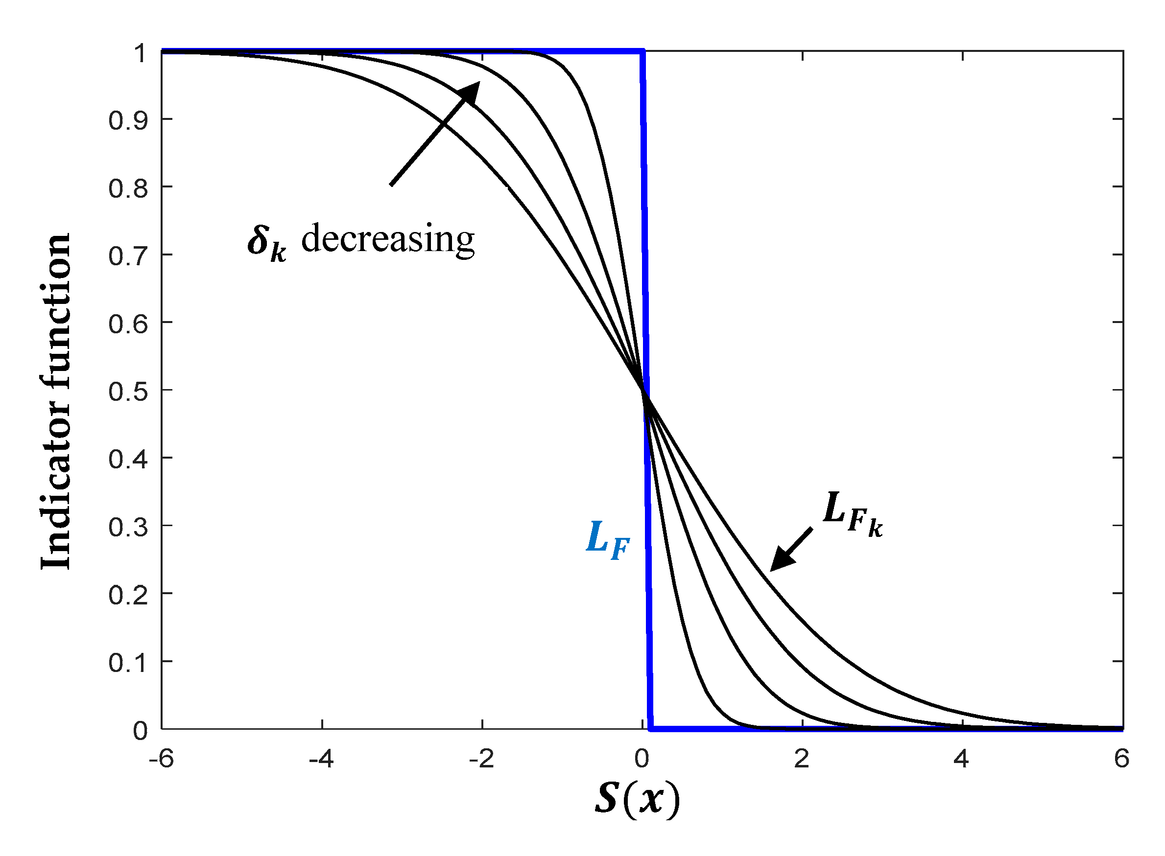
In the traditional CE-IM, the intermediate failure domain is identified by the intermediate failure threshold ${\zeta }_k$. Because of the step indicator function $L_{F_k}\left(x\right)$, ${\zeta }_k$ represents only a fraction ($\theta \in \left[0.01, 0.1\right]$) of the samples of the preceding ISD $q\left(x;u_{k-1}\right)$, and the other samples are neglected. In the ECE-IS, the indicator failure function of the intermediate failure events $L_{F_k}\left(x\right)$ is defined by a smooth approximation function. This allows a smooth transition for the approximately optimal ISD $q_k{}^{*}\left(x\right)$ towards the optimal ISD of the destination failure event $q^{*}\left(x\right)$ through exploiting all samples from the intermediate density $q\left(x;u_{k-1}\right)$ in parameter $u_k$ updating.

The indicator failure function can be defined as follows: $L_{F_k}\left(x;{\delta }_k\right)=\underset{{\delta }_k \to 0}{\lim }\Phi \left(-\frac{S\left(x\right)}{{\delta }_k}\right)$, where ${\delta }_k$ is the control parameter of function bandwidth, and $\Phi$ is the standard normal CDF. When ${\delta }_k$ approaches zero, the smooth function approaches to the target step indicator function. Hence, ${\delta }_0>{\delta }_1>\cdots >{\delta }_{NT}>0$ defines a decreasing series of bandwidths, as shown in Figure 3.

Using the smooth function of $L_{F_k}$, the optimization problem (20) becomes as follows:

$$u_k\underset{u_k}{=\mathrm{argmax}}\left[\frac{1}{N}{\displaystyle \sum }_{i=1}^N{W}_k\left(x_i;u_{k-1}\right)\ln (q\left(x_i;u_k\right))\right],$$

(22)

in which $W_k\left(x;u_{k-1},{\delta }_k\right)≔\frac{\Phi \left(-\frac{S\left(x\right)}{{\delta }_k}\right)g\left(x;w\right)}{q\left(x;u_{k-1}\right)}$. ${\delta }_k$ is determined such that the optimal ISD $q_k{}^{*}\left(x\right)$ is approximated well enough by samples drawn from $q\left(x;u_{k-1}\right)$, i.e., the variance of the importance weights $W_k\left(x;u_{k-1},{\delta }_k\right)$ is small. This is done by minimizing the difference between the $\mathbb{C}\mathbb{V}$ of the weights $\left\{W_k\left(x_i;u_{k-1},{\delta }_k\right),i=1,\dots ,N\right\}$ and the specified $ℂ{\mathbb{V}}_{target}$ at each intermediate event $k$, as written in (22).

$${\delta }_k=\underset{{\delta }_k\in \left(0,{\delta }_{k-1}\right)}{\mathrm{argmin}}\left|ℂ{\mathbb{V}}_{W_k}-ℂ{\mathbb{V}}_{target}\right|.$$

(23)

As shown in Algorithm 1, starting with ${\delta }_0=\infty$ and $u_0$ as a nominal parameter vector, this procedure is reiterated and stopped when the $ℂ\mathbb{V}$ of the weights calculated in (24) of the present smooth approximation of the optimal ISD of intermediate failure events with regard to the target optimal ISD is lower than the $ℂ{\mathbb{V}}_{target}$. Hence, $NT$ is set to the current event $k$, and the optimal ISD is approximated well enough by the density $q\left(x;u_{NT-1}\right)$. Utilizing the $ℂ\mathbb{V}$ of the weights as stopping criterion instead of the parametric density $q\left(x;u_{k-1}\right)$ improves the robustness of the method convergence, as will be shown in the section of results.

$$\left\{W\left(x_i;{\delta }_k\right)=\frac{q^{*}\left(x_i\right)}{q_k{}^{*}\left(x_i\right)}=\frac{L_F\left(S\left(x_i\right)\right)}{\Phi \left(-\frac{S\left(x_i\right)}{{\delta }_k}\right)},i=1,\dots ,N\right\}.$$

(24)

The samples from the density $q\left(x;u_{NT-1}\right)$ will be used in the second stage as shown in Algorithm 1 for computing the system adequacy indices (LOLP-EPNS) for each node and system. The system LOLP and EPNS can be expressed as follows:

$$LOLP=\frac{1}{N}{\displaystyle \sum }_{i=1}^N{L}_F\left(x_i\right)W\left(x_i;u_{NT-1}\right),$$

(25)

$$EPNS=\frac{1}{N}{\displaystyle \sum }_{i=1}^N\left({\displaystyle \sum }_{d=1}^n{L}_{curt.d}\left(x_i\right)\right)W\left(x_i;u_{NT-1}\right).$$

(26)

For nodes, the LOLP and EPNS can be rewritten as follows:

$$LOLP=\frac{1}{N}{\displaystyle \sum }_{i=1}^N{L}_F^d\left(x_i\right)W\left(x_i;u_{NT-1}\right),$$

(27)

$$EPNS=\frac{1}{N}{\displaystyle \sum }_{i=1}^N\left(L_{curt.d}\left(x_i\right)\right)W\left(x_i;u_{NT-1}\right),$$

(28)

in which

$$L_F^d\left(x_i\right)=\{\begin{array}{c}1 \mathrm{for} L_{curt.d}\left(x_i\right)>0\\ 0 \mathrm{for} L_{curt.d}\left(x_i\right)=0\end{array}$$

Algorithm 1. Procedure of adequacy indices assessment using ECE-IS

4. Results

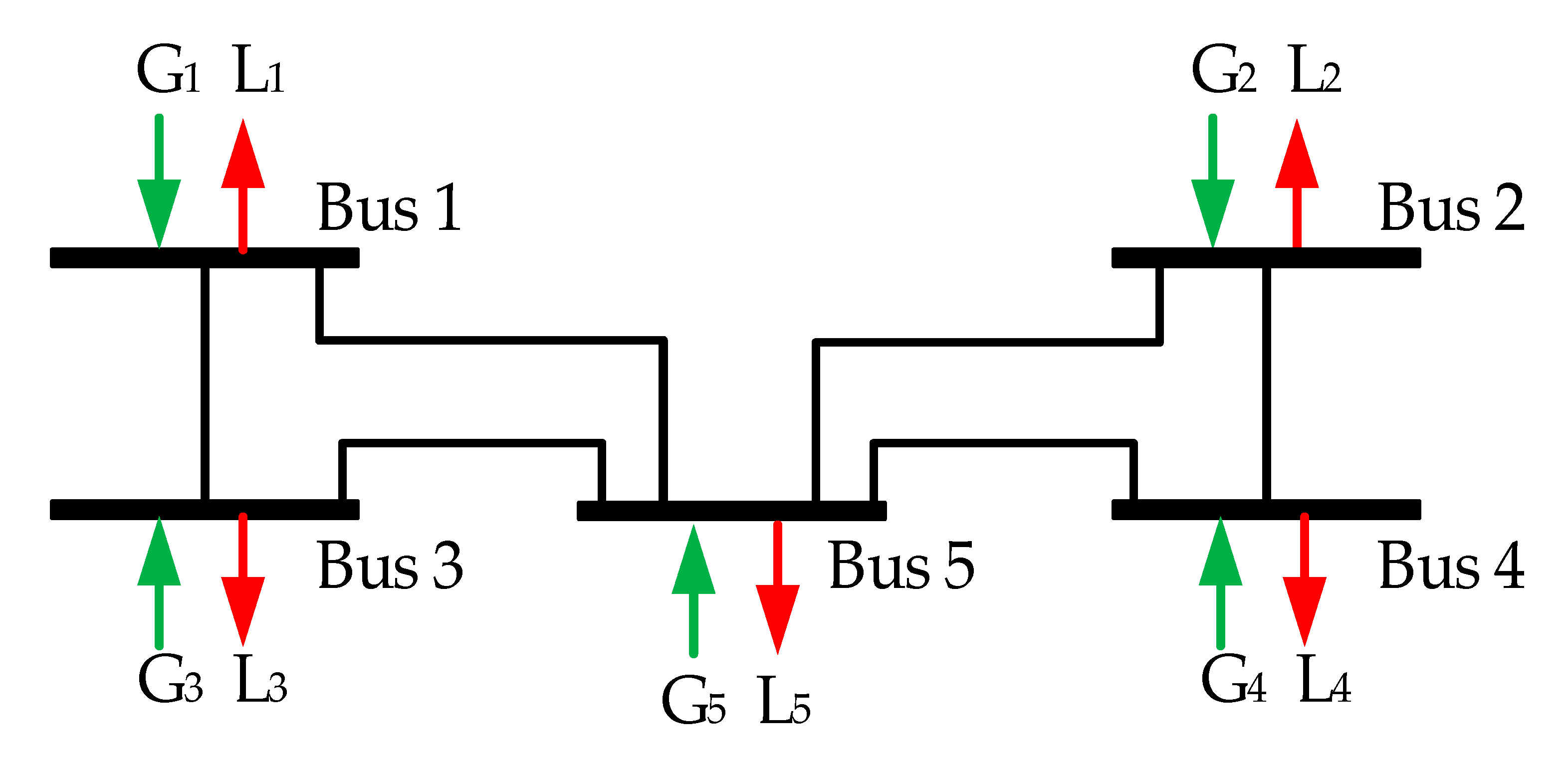
The proposed method is tested and evaluated for the five-bus test scheme, presented in Figure 4. The data for the buses and transmission lines are presented in

Table 1. Test scheme data.

Nodes Data					Transmission Lines Data
Bus	Available Generation (MW)		Load Demand (MW)		From	To	Resistance (Ohm)	Reactance (Ohm)	Capacity (MW)
					Bus	Bus
	Mean	STD	Mean	STD	1	5	10	100	500
1	1700	170	600	60	1	4	5	50	500
2	50	5	50	5	2	3	1	10	500
3	1440	144	900	90	2	4	3	33	500
4	1200	120	1500	150	3	4	2	10	500
5	1500	150	2000	200	4	5	5	50	500

. In terms of mean values of the generation and demand capacities, the test scheme includes two in surplus, one in balance, and two deficient buses. The probabilistic nature of the generation and demand could potentially result in different combinations of operational states of the power system buses. All the buses are connected by transmission lines of the same transmission capacity but different resistance and reactance. All tests are carried out using MATLAB 2017 on an Intel Core i5-8 G memory personal computer. The standard MCS simulation method is used as a benchmarking method. The maximum number of simulation samples for MCS is 5 × 10⁴. A coefficient of variation (convergence) of 5% for both system adequacy indices (LOLP-EPNS) is used as the stopping criterion. The rare events simulation techniques (CE-IS [33], SIS [35], SS [16], ECE-IS) use the following parameter values: $\theta =0.1,ℂ{\mathbb{V}}_{target}=0.05$, maximum number of iterations = 50, and number of samples per iteration = 2000.

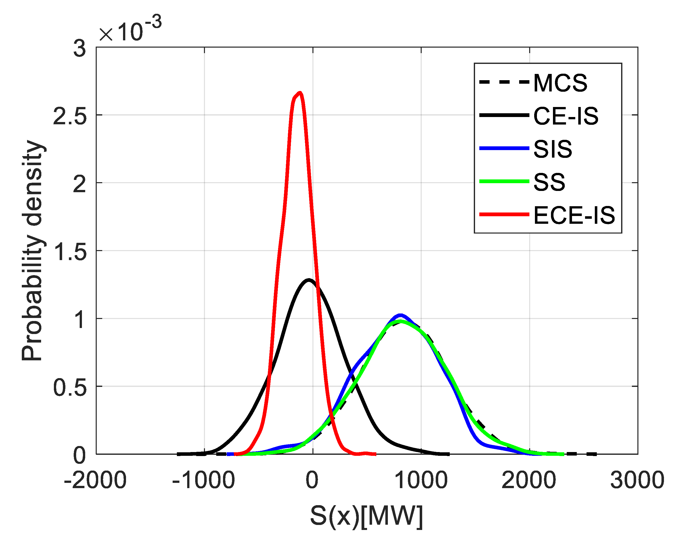
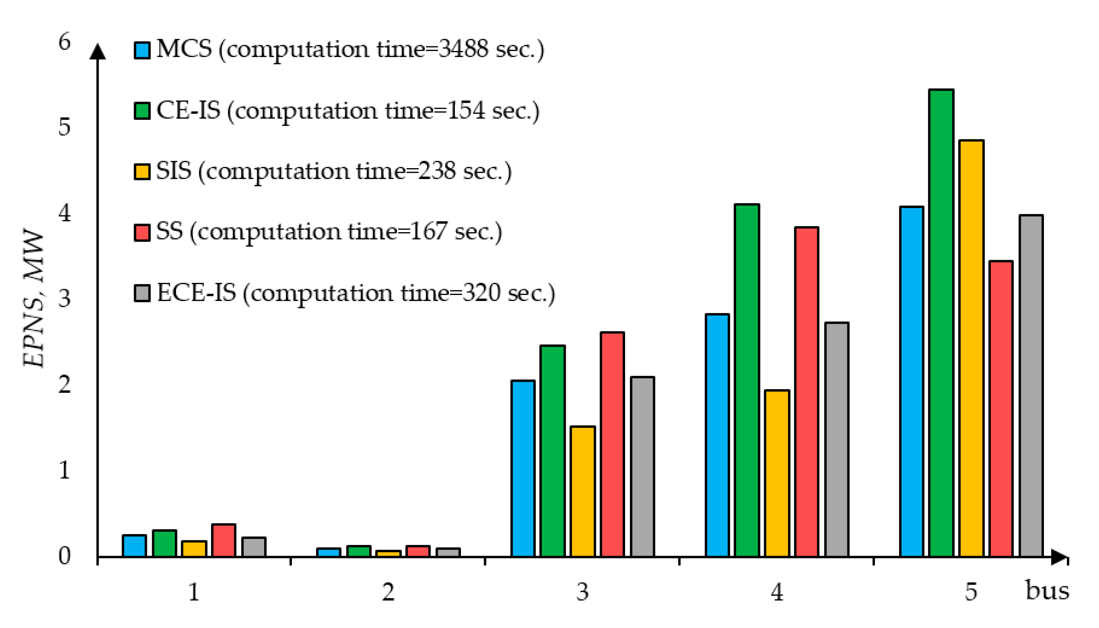
In Figure 5, the PDFs of the system limit-state function $\mathrm{S}\left(\mathrm{x}\right)$ are shown for different methods (CE-IS, SIS, SS, ECE-IS) and MCS. It illustrates that the proposed ECE-IS method has the largest probability of $\mathrm{S}\left(\mathrm{x}\right)<0$, which is 80% in comparison with 23, 55, 32, and 20% for MCS, CE-IS, SIS, and SS, respectively. This means that the samples extracted by the ECE-IS method are more likely to cause the load curtailment events. It represents 80% of the total sampled system states. Once the samples from the optimal distributions of nodal generations and loads are obtained, the adequacy indices (EPNS, LOLP) can be evaluated. For test purposes the EPNS, LOLP are calculated for all the buses. The histogram in Figure 6 shows the computation time and the EPNS values obtained by the different methods. The computation time includes the time spent in the first stage for extracting the rare load curtailment events.

The load curtailment sharing philosophy results in relatively small EPNS values of potentially deficient buses 4 and 5. At the same time, the limited transmission lines capacity does not allow unlimited power supply from surplus buses and so the greatest EPNS is at bus 5. From the simulation results, it became clear that all the discussed methods significantly reduce a computation burden and the most computationally effective is the CE-IS method. It also could be seen that the method used in extracting load curtailment events could significantly affect results. 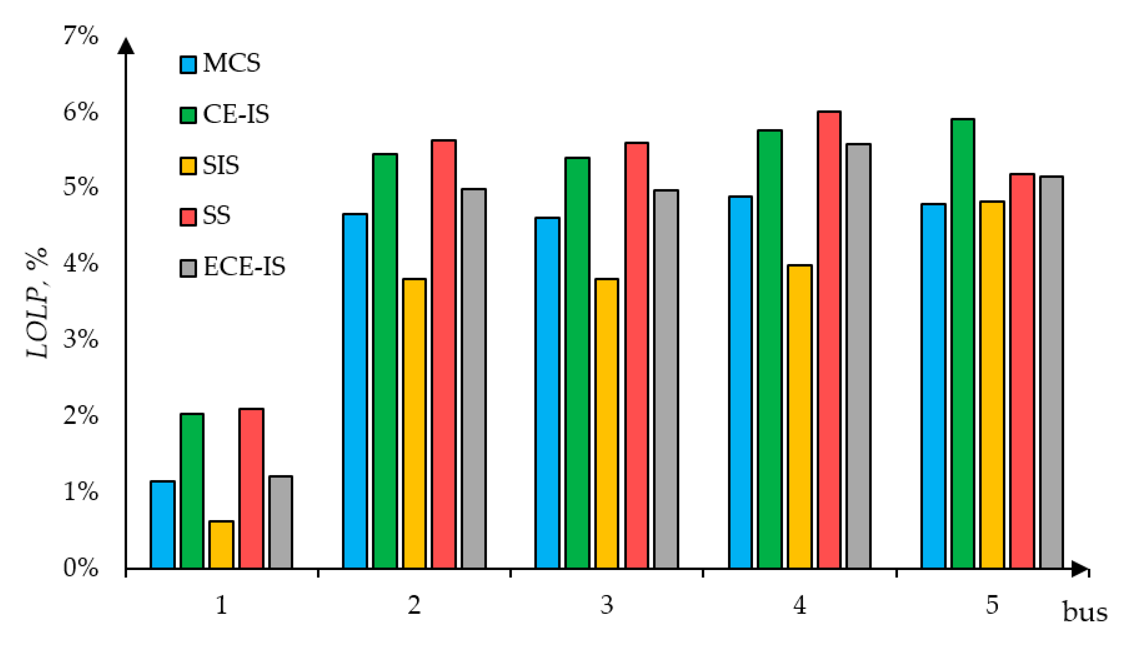Figure 7 shows the LOLP values for all the busses of the test scheme. Theoretically, in the case of unlimited transmission lines capacity, the objective function (1) must result in equal LOLP of all the buses. However, in terms of mean values, the power surplus of the bus 1 is 10% higher than the transmission capacity of the connected lines. Possible power supply from bus 1 is locked, and as a result, in some deficient test scheme state samples, the demand at the bus is not curtailed. It can be seen from the histogram that the LOLP of bus 1 is relatively small in comparison to other bus values. 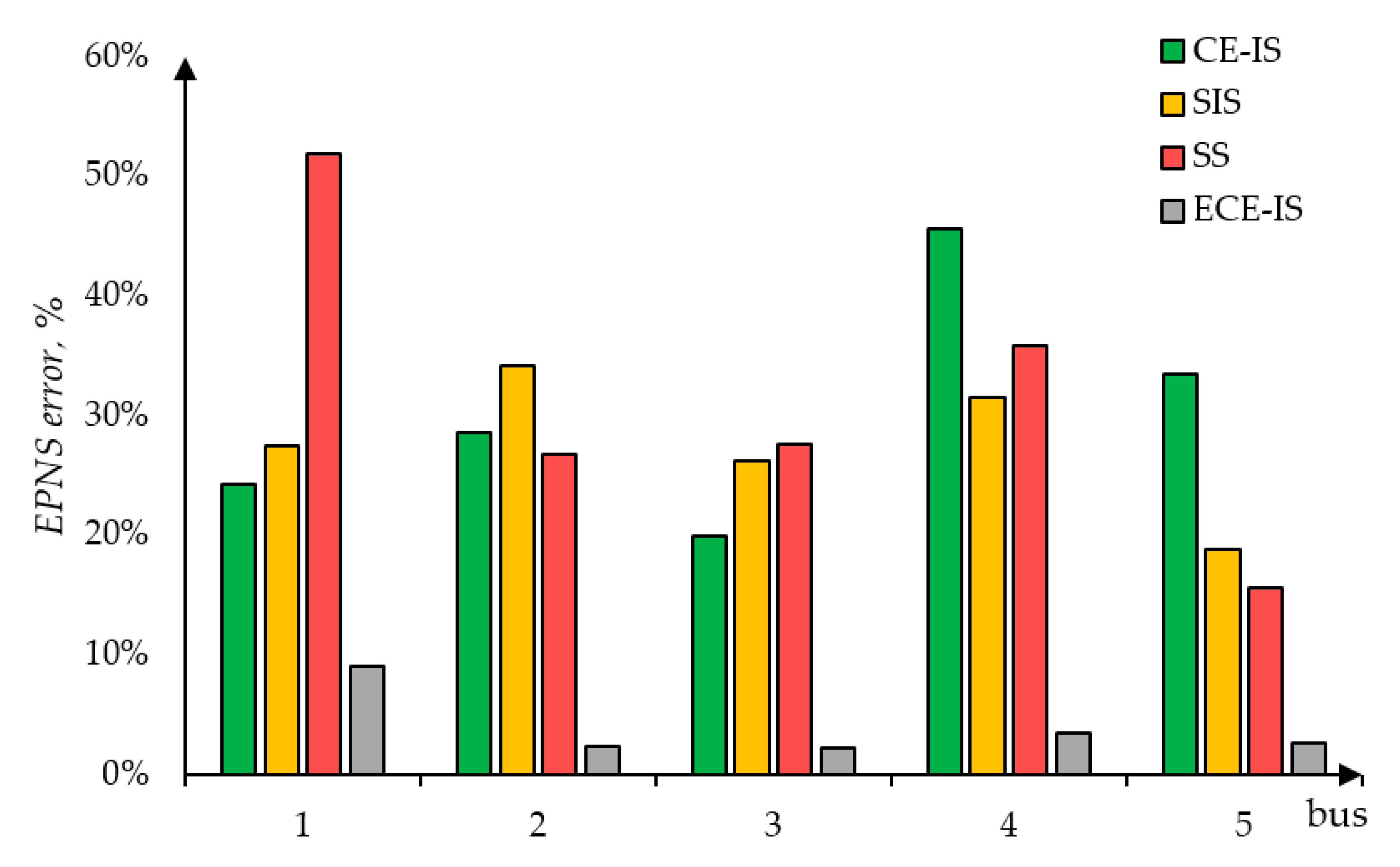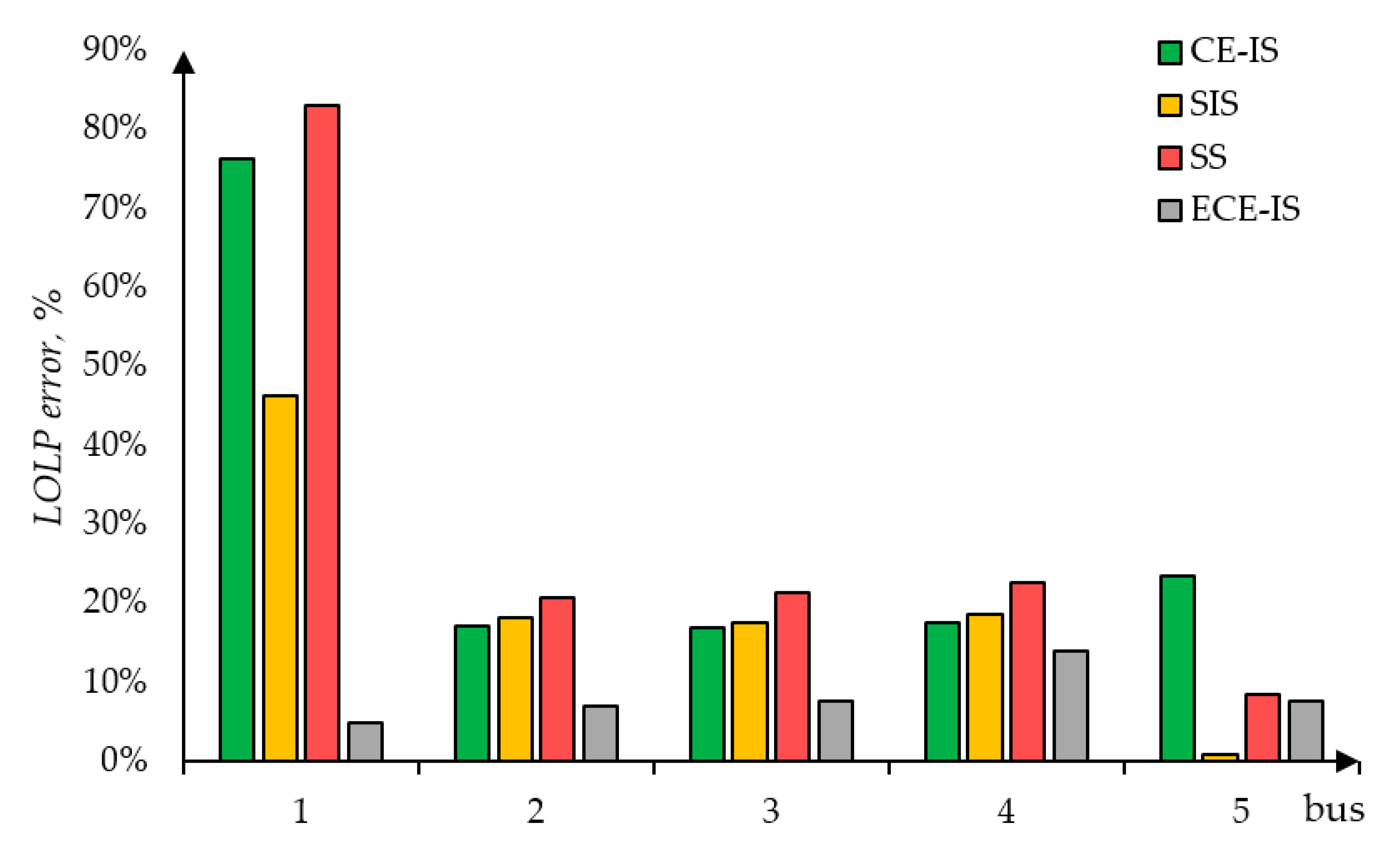Figure 8 and Figure 9 show the errors of methods in comparison to the standard MCS method. For almost all the buses, EPNS values computed using the proposed method are accurate within range of 8%. Even though the ECE-IS method is less computationally effective than other methods, it could provide significantly more accurate results. In comparison to the traditionally used MCS approach, the proposed method is nearly eleven times faster. The smallest LOLP error values are generally also represented by the ECE-IS approach. Notice, that in the case of LOLP, even small deviations would introduce a great error, as it can be seen.

5. Discussion

A trade-off between the computational accuracy and computational efficiency leads to a wide number of approaches for a power system adequacy evaluation. Therefore, the comparison among methods must include the number of samples or computation time required to reach the accurate adequacy indices with acceptable convergence. In terms of the number of samples, the system LOLP and EPNS indices and their convergence using the standard MCS method and the different rare events simulation approaches are shown in Figure 10, Figure 11, Figure 12 and Figure 13. For MCS, the number of samples to reach a convergence of 5% for both system LOLP and EPNS indices is 38,945 samples. The CE-IS and SS methods have the fastest convergence rate, while they do not develop accurate LOLP values. The ECE-IS has performed better, reaching a 0.0099 LOLP value with 4.7% convergence and 8.95 MW EPNS with 2.4% convergence. On the other hand, the standard MCS has achieved 0.0102 with 5% and 8.8 MW with 2.5% for LOLP and EPNS, respectively. Therefore, the ECE-IS can achieve the same accuracy of the standard MCS method for both nodal indices, as shown in Figure 8 and Figure 9, and system indices, as shown in Figure 10 and Figure 12. In the attitude of computational efficiency, the ECE-IS needs seven iterations for extracting 2000 samples representing the load curtailment events, and so, the total number of samples is 14,000 samples. Hence, the ECE-IS can achieve accurate results with a smaller number of samples and computation time. As shown in Figure 6, an 11-times speedup is achieved.

For comparing the robustness of the ECE-IS method with other rare events simulation techniques, the system LOLP, LOLP relative bias, and LOLP convergence values are illustrated in

Table 2. Methods comparison for different numbers of samples.

Number of Samples per Iteration	Methods	Number of Iterations	System LOLP	Relative Bias of System LOLP	System LOLP Convergence	Time [sec]
250	CE-IS	3	0.0329	2.2	0.35	19
	SIS	4	0.023	1.25	0.59	30
	SS	3	0.0613	5	0.52	21
	ECE-IS	8	0.012	0.17	0.21	43
1000	CE-IS	3	0.0219	1.14	0.055	96
	SIS	5	0.0038	-0.63	0.44	106
	SS	3	0.041	3	0.064	85
	ECE-IS	8	0.0114	0.12	0.085	140
2000	CE-IS	3	0.0191	0.87	0.045	154
	SIS	4	0.0052	−0.49	0.20	238
	SS	3	0.0272	1.67	0.042	167
	ECE-IS	7	0.0099	0.03	0.048	320

for different numbers of samples per iteration. The sample analyzing times differ from each other; hence, the computation time is included in Table 2. Taken the LOLP value (0.0102) obtained by the standard MCS method as a reference value, the relative bias of LOLP values is computed as follows: $\frac{LOLP-LOLP\left(MCS\right)}{LOLP\left(MCS\right)}$. From the results in Table 2, the convergence acceleration for all methods is achieved by increasing the number of samples. However, there is a significant accuracy loss with a small number of samples for CE-IS and SS methods, while the SIS achieves a proper LOLP bias at 1000 samples but bad convergence. However, the ECE-IS is still effective for a small number of samples. It achieves a small LOLP bias (17%) with 21% convergence at 250 number of samples.

In order to verify the computation accuracy and efficiency of the proposed method with the dimension of the power network and the number of random variables being considered, the results of adequacy indices are presented for the IEEE-RTS 79 system. The system includes 24 buses and 32 generators divided among 14 generating stations totalizing 3405 MW of installed capacity. The annual system peak load is 2850 MW. More information on the IEEE-RTS 79 can be found in [40]. The mean and standard deviation values for the loads were taken at the peak value and the $\pm 10\%$ of the peak value, respectively. A coefficient of variation (convergence) of 5% for both system adequacy indices (LOLP-EPNS) is used as the stopping criterion. For the ECE-IS and MCS methods,

Table 3. System adequacy indices for IEEE-RTS 79.

Methods	Number of Samples	System LOLP	System EPNS [MW]	Time [sec]
MCS	382,000	0.00119	0.154	6220
ECE-IS	87,000	0.00121	0.16	810

shows the results of the system LOLP and EPNS indices, number of samples, and computation time. The computation time includes the time spent in the first stage for extracting the rare load curtailment events. The results of the ECE-IS method are 0.00121 and 0.16 MW for LOLP and EPNS, respectively. On the other hand, the standard MCS has achieved 0.00119 and 0.154 MW for LOLP and EPNS, respectively. Therefore, the ECE-IS can achieve the same accuracy of the standard MCS method for both system indices. Moreover, the ECE-IS method is considerably more efficient than the standard MCS method. The proposed method needs only a small fraction (23%) of the samples needed by the MCS. However, in contrast to MCS, the ECE-IS method, as other techniques of rare events simulation, come along with its own set of tuning parameters, which are the target the coefficient of variation of importance weight function and the number of samples per iteration. The proper tuning of these parameters has consequences on the efficiency of the technique.

6. Conclusions

In this paper, a framework of adequacy indices evaluation has been proposed in composite generation and transmission power systems. The main purpose of the framework is to obtain accurate adequacy indices and enhance the computational efficiency of the standard MCS method. This is achieved by integrating rare events simulation methods in the framework’s first stage for identifying the approximately optimal distortion of the nodal generations and load distributions, making rare load curtailment events more likely to be drawn. As a result of the integration of the rare event simulation methods, a new approach named ECE-IS is proposed that is more efficient and robust than other methods, such as traditional CE-IS, SIS, and SS in extracting the optimal distortion. From the reported results of the framework’s second stage, the proposed method contributes to accurately evaluating the adequacy indices (LOLP-EPNS) and further enhancing the convergence of the indices in comparison with other methods. Moreover, a great speed-up was shown in terms of computation time with respect to the standard MCS method.

The implementation of the proposed method in adequacy evaluation could allow us to use more detailed power system models, which would more accurately reflect real power system operation. The impact of different network topologies (i.e., transmission network contingencies), non-linearity of the power flow equations, and chronological characteristics of power systems, such as time and spatially correlated load models, the time-dependency of renewable energy resources could be included into the power system model. This method can also be included into the many problems in both operation and planning phases, such as the evaluation of spinning reserve margins and the integration of renewable energy resources. Using adequacy indices assessments and knowing the critical nodes during system disturbance, planners can better manage the penetration of renewable sources, ensuring sustainable and reliable operation at both the system and nodal level. In the context of power system operation, operators schedule the generating units and allocate enough generation reserve amounts to ensure a lower adequacy index (the probability of load curtailment) than the maximum allowed. These issues will be adopted in future works.