Design of Fractional Order Controllers Using the PM Diagram

Abstract

This work presents a modeling and controller tuning method for non-rational systems. First, a graphical tool is proposed where transfer functions are represented in a four-dimensional space. The magnitude is represented in decibels as the third dimension and a color code is applied to represent the phase in a fourth dimension. This tool, which is called Phase Magnitude (PM) diagram, allows the user to visually obtain the phase and the magnitude that have to be added to a system to meet some control design specifications. The application of the PM diagram to systems with non-rational transfer functions is discussed in this paper. A fractional order Proportional Integral Derivative (PID) controller is computed to control different non-rational systems. The tuning method, based on evolutionary computation concepts, relies on a cost function that defines the behavior in the frequency domain. The cost value is read in the PM diagram to estimate the optimum controller. To validate the contribution of this research, four different non-rational reference systems have been considered. The method proposed here contributes first to a simpler and graphical modeling of these complex systems, and second to provide an effective tool to face the unsolved control problem of these systems.

1. Introduction

Most typical diagrams used in control engineering, such as the root locus, the Bode plot, the Ziegler–Nichols method, or the Nyquist plot, show partial aspects of the Transfer Function (TF). In all of them, it is possible to extract some characteristics of the system and to design different types of controllers to improve the system behavior. Nowadays, with tools such as MATLAB Control System Designer app https://es.mathworks.com/help/control/ref/controlsystemdesigner-app.html (previously called SISO Design Tool), it is possible to compare many of these diagrams at the same time together with the time response of the system and the parameters required to tune the controller. However, they do not contain a complete representation of the TF. In addition, the basic version of these diagrams is only useful when the system to be controlled presents a rational structure. Because of this, the aim of this work is to represent systems given by their TFs in a different (graphical) way and to find other possible applications from this graphical representation.

TFs are complex functions where the input and the output are represented by two variables. Therefore, it is necessary to have four axes to represent them. The input corresponds to a complex number where the variables are the real and the imaginary component and the output is divided into magnitude and phase. The Phase Magnitude (PM) diagram is an intuitive tool that makes it easier to comprehend these functions. Our brain is trained to visualize objects in three spatial dimensions, and it is not easy to understand graphs in a four-dimensional space. As said in [1], complex functions have the reputation of being mysterious entities. Seeing these strange objects may help to overcome the fear one might feel while dealing with them. This new representation can help researchers and students in their daily work.

In some papers [2,3] and books [1,4,5,6] about complex variables, the researchers have represented complex functions in many ways that include colors to incorporate the phase. The problem of these approaches is that the representations do not permit obtaining accurate measurements.

A previous work by the authors of this paper [7] developed a tool called PM diagram that is easy to implement and contains all the information of the TF. Its main characteristic is that the magnitude and the phase of the TF can be visually identified in a simple graph. This tool was intuitively applied to design multiple different controllers for rational systems. The method relies on the classic control approaches (root locus, Bode, etc), but the starting point is a visual identification of the magnitude and phase that have to be added by the controller in order to meet the design specifications, which makes this technique a very intuitive method for the engineer. In addition, the graphical representation allows us to understand the behavior of the function, which is more difficult if only the equation is available. These facts let us consider this technique as a promising option when investigating different methods to control more complex systems.

As will be demonstrated in this paper, this tool is especially useful when applied to non-rational systems. Instead of applying complicated techniques, the same simple ideas can be applied for the design of PM-based controllers.

Once the PM diagram of the system has been plotted, any control method can be applied. In our case, our control technique is based on the use of a fractional order Proportional Integral Derivative (PID) controller. These types of controllers are a generalization of PID controllers proposed by Podlubny [8], where the integrator order $\lambda$ and the differentiator order $\mu$ assume real non-integer values. For this reason, the usual notation is PI${}^{\lambda }$D${}^{\mu }$. Since five parameters can be tuned, more specifications can be met. Due to its flexible structure in comparison with other conventional controllers and considering the non-rational character of the TF, this PI${}^{\lambda }$D${}^{\mu }$ controller is a perfect candidate for the validation of the present proposal. This controller will be used to demonstrate to what extent the PM approach can be applied for more complex systems and to deeply discuss its performance as a control method.

In a previous work [9], evolutionary computation concepts were applied to tune the parameters of PI${}^{\lambda }$D${}^{\mu }$ controllers in order to meet the requirements for a Direct Current (DC) motor modeled by a second order linear differential equation. The Differential Evolution (DE) algorithm is used to optimize the parameters of the controller [10]. This technique is a population-based algorithm where each member of the population is a possible solution (fractional order PID) to the optimization problem. A fitness function is defined for each candidate to recognize the worth of each possible solution. The population set evolves according to a fitness value to the optimum solution, which is the best controller according to the system and the fitness function. This methodology is expanded here to control more complex systems.

This paper presents a modeling and control technique for the tuning of a fractional order PID controller for non-rational systems where the PM diagram is the tool that the DE-based method uses to estimate the optimum controller. Four different systems from well-known literature with non-rational TFs have been chosen to test the behavior of the method. As will be demonstrated in the experiments, satisfactory results are obtained in all cases, demonstrating that the method proposed contributes first to a simpler and graphical modeling of these complex systems, and second to provide an effective tool to face the unsolved control problem of these systems.

The main innovation of this work is summarized next:

• The PM approach can be applied for the modeling and control of any kind of rational and non-rational system represented by a TF.
• In comparison to other approaches in the literature, the PM tool provides a more complete representation of the TF, which makes it an interesting technique to be used in control systems’ education.
• Its graphical nature makes it simple and intuitive to use.

This work is structured as follows. The PM diagram is detailed in Section 2. After that, the most important concepts about fractional order PID controllers are explained in Section 3. Section 4 contains implementation details of the tuning method. The systems that will be tested are introduced in Section 5. Then, the experimental results are presented in Section 6. Finally, the conclusions are summarized in Section 7.

For the sake of readability,

Table 1. Table of used acronyms and terms.

Acronym	Name	Meaning
PM	PM diagram	Phase Magnitude diagram
PID	PID controller	Proportional Integral Derivative controller
PI${}^{\lambda }$D${}^{\mu }$	Fractional order PID controller	Fractional order Proportional Integral Derivative controller
$M_{dif-PM}$	$M_{dif-PM}$	Magnitude added at the frequency of interest
$P_{dif-PM}$	$P_{dif-PM}$	Phase added at the frequency of interest
${\phi }_m$	Phase margin	Stability measurement
$A_{dec}$	Interval where the phase is intended to be flat	Robustness measurement
${\omega }_{cg}$	Gain crossover frequency	Gain crossover frequency
$T\left(j{\omega }_t\right)$	Complementary sensitivity function	High frequency noise rejection
$S\left(j{\omega }_t\right)$	Sensitivity function	Disturbance rejection
ISE	Integral of the Squared Error	Performance criterion in stability analysis
IAE	Integral of the Absolute Error	Performance criterion in stability analysis
HSV	Hue, Saturation, Value (or Brightness) of an image	Color model
RGB	Red, Green, Blue levels of an image	Color model

shows a list of the acronyms and main terms used in this paper.

2. Phase Magnitude Diagram

This section presents the graphical tool that has been implemented to make the tuning task easier for complex non-rational models. In the PM diagram, the variables that completely define the TF will be displayed: two of them correspond to the complex variables in the s-plane, and the other two are the magnitude and phase of the TF for a given complex number s.

The s-plane is represented by two axes, following the same notation used in other classical graphical tools such as the root locus.

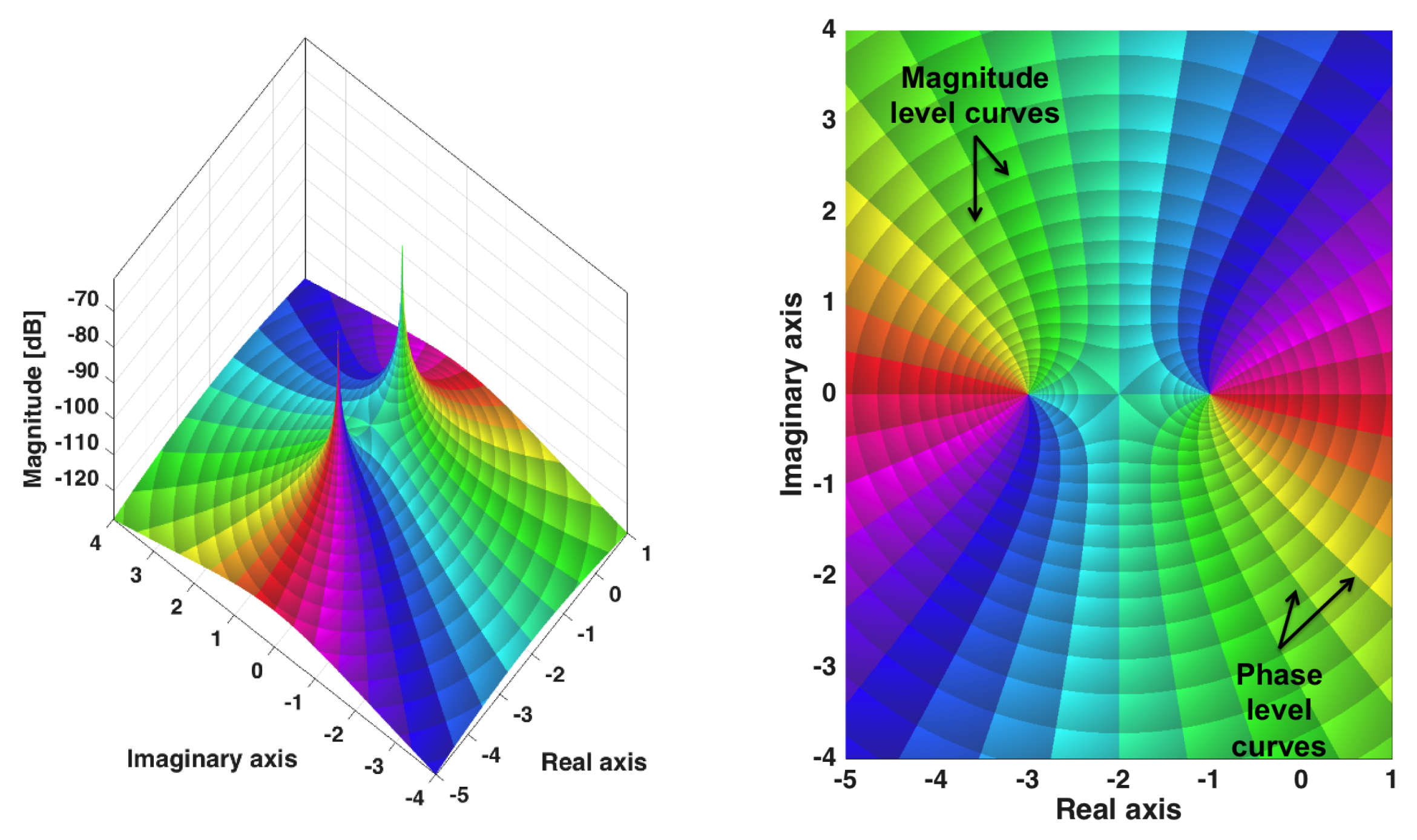
In order to completely depict a TF given by $G\left(s\right)$, the solution adopted by the PM approach utilizes level curves in a third dimension to identify the system magnitude, as can be seen in Figure 1. The function magnitude is represented in decibels:

$${\displaystyle {\left|G\left(s\right)\right|}_{dB}=20log\left|G\left(s\right)\right|,}$$

(1)

and level curves in a third dimension are used to compare points in the s-plane that share the same magnitude. This variable can be plotted in a three-dimensional graph or in a projection in a two-dimensional plane. The magnitude level curves are equally spaced in the diagram with increments of 2 dB.

The phase of the TF is the fourth variable to be extracted from the PM diagram and it is identified by colors. Color-coded values in the function domain are applied to show the phase of the TF for a given value in the s-plane. Therefore, another set of curves is used for $arg\left[G\right(s\left)\right]$. The scale is linear, with red representing $0^{\circ }$ and cyan being ${180}^{\circ }$. This means that the cyan line corresponds to the root locus and the red line is the inverse root locus. The Hue, Saturation, Value (HSV) color space is applied to represent the arguments. This space defines a color model in terms of its components. The colors begin with red ($0^{\circ }$), pass through yellow, green, cyan (${180}^{\circ }$), blue, magenta, and return to red (${360}^{\circ }$). The phases are also equally spaced with increments of ${20}^{\circ }$.

A simple example for $G\left(s\right)=1/(s+1)(s+3)$ can be observed in Figure 1. The three-dimensional view is shown in Figure 1 left. The s-plane is represented in the horizontal axis. The vertical axis and the corresponding level curves show the different magnitudes. The reader can check that the magnitude tends towards the infinity when s is $-1$ or $-3$, which are the poles of the open-loop system. Each point in the complex plane has an associated color.

The planar projection of the PM diagram is displayed in Figure 1 right. Observing the figure, the cyan lines correspond to the root locus and the red ones to the inverse root locus. The planar view of the PM diagram is more useful when designing controllers. This is mainly because it is very intuitive to read the magnitude and phase that are needed to obtain the poles in closed-loop required to meet the control specifications.

For example, imagine that the closed-loop poles of the actual system (without controller) are situated in $s=-2\pm 1.5j$ (right part of Figure 1). The requirements could be to obtain closed-loop poles in $s=-2.5\pm 2.5j$. The number of lines in the phase reference frame between $-2\pm 1.5$ and $-2.5\pm 2.5$ correspond to the phase that must be added by the controller ($P_{dif-PM}$). The same happens with the magnitude level curves, and the magnitude difference is called $M_{dif-PM}$.

In the classical control approaches based on the root locus diagram, the angle condition is applied to compute how the root locus has to be modified to contain the dominant poles. After that, the magnitude condition fixes the closed-loop poles in the desired positions. In this work, the same variables (magnitude and phase) can be intuitively obtained using the PM diagram and, after that, can be taken into account to meet the specifications. The classical method is limited to systems with rational TFs (linear systems modeled by linear differential equations), but the current approach can be applied to non-rational systems, which is an important advantage of this technique.

As observed from the figures, the PM diagram allows direct and graphical inspection of the system TF characteristics. After that, any control technique can be applied for the design of a controller for that system. For example, after reading the phase of $G\left(s\right)$, a controller $C_1\left(s\right)$ that adds that phase ($P_{dif-PM}$) with a gain of one can be calculated. Then, the PM diagram of $C_1\left(s\right)G\left(s\right)$ is represented and the gain that is needed ($M_{dif-PM}$) is used to compute the final expression of the controller $C\left(s\right)$. In this work, a fractional order PID controller and a DE-based tuning method that follow the same ideas presented in [9] are adopted. In this way, our previous work is expanded to include the design of controllers for non-rational systems. The main concepts about this control strategy are described in the next section.

The PM approach permits to study the time domain and the frequency domain responses at the same time. It is possible to draw a grid over the PM diagram in order to read values of other variables such as the damping ratio $\zeta$ or the natural frequency ${\omega }_n$. Figure 2 left shows these variables for the PM diagram of $G\left(s\right)$. It has to be said that the dashed lines drawn in the figure are only valid under the assumptions made for second-order linear systems. Different equations would be needed to draw the grids for different types of systems.

The PM diagram also allows us to read the phase margin directly because it is the phase distance (in number of lines, each line represents ${20}^{\circ }$) from the actual closed-loop poles to the imaginary axis following the same magnitude line. The gain margin is the magnitude distance between the closed-loop poles and the imaginary axis following the cyan line that represents ${180}^{\circ }$ (root locus). The imaginary axis represents the Bode plot. In the drawings, linear scales have been used for the real and imaginary axes, but if there are poles and zeros placed in different decades, it could be better to use logarithmic scales. An example is shown in the right part of Figure 2, where the phase and gain margins of the system are represented. Phases at different frequencies of the Bode plot can be directly read in the diagram (red dots). Note that a decade is a unit for measuring frequency ratios on a logarithmic scale, with one decade corresponding to a ratio of 10 between two frequencies (an order of magnitude difference).

Another advantage is that any kind of complex function can be represented, thus it is possible to model complex non-rational systems in a simple way.

The PM representation can be considered as a root contours plot with two parameters: gain and phase [11,12]. It is not the first time that level curves have been used to represent the magnitude and the phase of a function. A related approach can be found in the work by Cavicehi [2]. The main drawback of his approach is the bad resolution and the difficulty of reading.

Our technique has been successfully applied to design different controllers for rational systems in [7]. One of the main contributions of this paper is to expand this study to more complex systems. The real utility of this method is to develop an application to tune controllers for non-rational systems, where the control strategy is usually a challenge. From an educational point of view, non-rational systems are usually described using complicated concepts, and this approach is an additional resource that helps to understand the theory behind these systems in an easier way.

3. DE-Based Tuning of Fractional Order PID Controllers

The PM technique detailed in this paper can be used to tune multiple types of controllers. Due to our previous experience [13,14], a fractional order PID controller, where the parameters are optimized using the DE algorithm, has been chosen. A real application to control a DC motor has been presented in [9] following this control approach. This same tuning method is applied here to control non-rational systems utilizing the PM diagram. The main procedure is summarized in this section.

As said before, PI${}^{\lambda }$D${}^{\mu }$ controllers are a variation of the classical PID controllers with non-integer orders for the integrator and the differentiator. This type of controller was first developed by Podlubny [8]. In [15], the same research group demonstrated that these controllers present better control performance. An introduction to these fractional order controllers is given in [16].

A $P{I}^{\lambda }{D}^{\mu }$ controller is given by the following equation:

$$C\left(s\right)=k_p+\frac{k_i}{s^{\lambda }}+k_d{s}^{\mu },$$

(2)

where $k_p$, $k_i$, and $k_d$ are the proportional, integral, and derivative gains of the typical $PID$ controller; and $\lambda$ and $\mu$ are the fractional orders of the integral and derivative parts of the controller, respectively. When compared to the classic approach, the user has two more parameters to tune in this type of controller ($\lambda ,\mu$), which implies that more control requirements can be satisfied.

The appearance of this new type of controller caused that many researchers focused on the design of new effective tuning methods for non-integer order controllers, while others focus on the solution of fractional differential equations [17,18,19]. An exhaustive classification of these tuning techniques can be found in [20]. The authors defined three different groups: analytical, rule-based, and numerical.

The analytical methods can be applied to systems defined by a low number of simple equations. For example, Vinagre [21] assumes that $\lambda$ = $\mu$ to develop a procedure where all parameters can be analytically derived by solving four nonlinear equations based on the gain crossover frequency, phase margin, phase crossover frequency, and gain margin specifications. Chen et al. [22] have implemented a method for fractional PI controllers where the requirement is the robustness to loop gain variations. This specification is used together with the gain crossover frequency and phase margin to design fractional order PID controllers in [23,24,25]. In [26], the authors propose fractional-order lead/lag compensators. The rule-based methods rely on some tuning rules [27,28,29]. Their limitation is that the process should usually be a system having an S-shaped step response. The numerical methods apply optimization-based techniques. Chen et al. [30] have developed an F-MIGO algorithm for tuning fractional PI controllers. A nonlinear optimization problem with five constraints is solved in our previous work [31] for tuning the fractional order $P{I}^{\lambda }{D}^{\mu }$ controller. In [32], the controller is designed taking into account the robustness property with respect to time-constant variation and the phase margin.

A new strategy to estimate the parameters of a fractional $P{I}^{\lambda }{D}^{\mu }$ controller that meets some specifications for a given plant was proposed in [9]. It relies on the DE algorithm, which is an evolutionary optimization technique that minimizes a fitness function. Given a process with a known TF $G\left(s\right)$, the DE-based algorithm calculates the parameters of the fractional controller $C\left(s\right)$ in order to satisfy several specifications in closed-loop. An open-loop TF equal to $C\left(s\right)G\left(s\right)$ and negative unity feedback are assumed. Two different cost functions were designed depending on the requirements to be met: the first one is defined in the time domain and it minimizes the error between the output and the reference input; the second one satisfies some specifications in the frequency domain, including robustness to gain variations of the plant. The second cost function in the frequency domain is considered here. This strategy, which is applied together with the PM diagram, is described below.

The DE optimizer is a population-based algorithm, which means that there is a population set where each member is a possible solution to the optimization problem. The $P{I}^{\lambda }{D}^{\mu }$ controller is formed by five parameters, as described in (2): three corresponding to the gains and two representing the exponents. Therefore, each candidate solution has five parameters: $k_p$, $k_i$, $k_d$, $\lambda$, and $\mu$. The first step of the tuning method is to define the initial population, which is generated randomly but taking into account the search space. The search space has to be limited to have a reasonable computational time. Otherwise, population requirements would be huge.

The cost value has to be computed for each population member. This variable is the key of the method because this is the parameter which is optimized. The PM diagram is applied to implement a fitness function in the frequency domain where the objective is to obtain a flat phase of the open loop system under several constraints. This strategy is explained at the end of this section.

The optimization filter consists of an iterative process that is executed until the convergence conditions are met. In each iteration, the new population for the next generation is created. The population set (controller parameters) evolves in time to minimize the fitness value. The evolutionary mechanism is formed by three different operations: mutation, crossover, and selection. First, each candidate of the current population is perturbed to generate a mutated vector. After that, the crossover stage increases the diversity of the new generation by combining parameters of the current population and the mutated vector. The population set of the next generation is chosen according to a selection mechanism that compares the new candidates to the current members. If the fitness value of the proposal is better than the fitness value of the current member, then it is replaced by the new candidate. Otherwise, the current member is maintained for the next generation. The previous process (mutation, crossover, and selection) is applied to the whole population, obtaining the next generation population.

After convergence, the solution is the candidate with the best fitness value. This solution represents the $P{I}^{\lambda }{D}^{\mu }$ controller that minimizes the cost function.

Fitness Function

If the fitness function is defined in an adequate way, the DE optimizer can obtain the solution sooner for a given problem. An important advantage of the evolutionary filter with respect to the classical approaches is the flexibility of the tuning strategy because many different functions could be tested and implemented. The objective here is to compute the optimum $P{I}^{\lambda }{D}^{\mu }$ controller for a non-rational system using the PM diagram. Since the Bode plot corresponds to the imaginary axis in this diagram, a cost function in the frequency domain has been selected.

The classical methods take into account five different constraints because five parameters can be tuned in the $P{I}^{\lambda }{D}^{\mu }$ controller [31]. An advantage of this evolutionary strategy is that more specifications could be met if they can be implemented in the cost function.

In control engineering, one of the most demanding specifications is the robustness to variations in the gain of the plant [33,34], which is equivalent to obtain a flat phase:

$${\left.\frac{d\left(arg\right(F\left(s\right)\left)\right)}{d\omega }\right|}_{\omega ={\omega }_{cg}}=0,$$

(3)

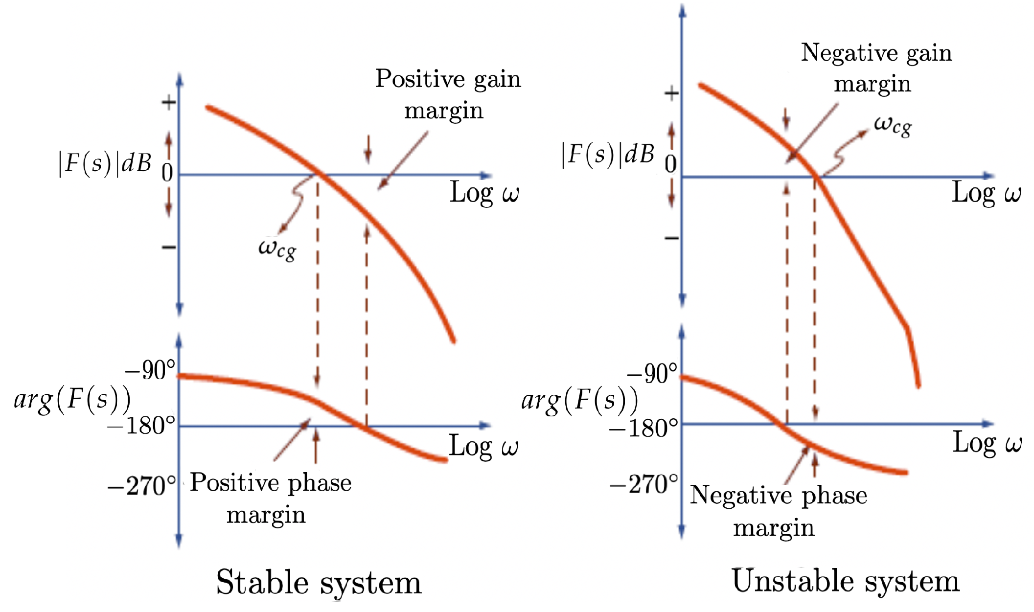
where ${\omega }_{cg}$ is the gain crossover frequency (the frequency at which the magnitude of the open-loop system is 0dB) and $F\left(s\right)=C\left(s\right)G\left(s\right)$ is the open-loop transfer function (see Figure 3 for the representation of the magnitude and phase of the open-loop system as a function of the frequency). A flat phase within an interval around ${\omega }_{cg}$ implies that the system will be more robust to gain changes and the overshoot of the response is almost constant within a gain range, which is called the iso-damping property of the time response.

The fitness value is computed for each possible $P{I}^{\lambda }{D}^{\mu }$ controller according to the next equation:

$$fitness\left(i\right)=\sum _{\omega ={\omega }_i}^{{\omega }_f}{(\phi \left(\omega \right)-\phi \left({\omega }_{cg}\right))}^2,$$

(4)

where the phase differences are calculated in an interval between ${\omega }_i$ and ${\omega }_f$ around the gain crossover frequency. $\phi \left(\omega \right)$ is the phase of the open-loop system at a frequency $\omega$.

Several constraints have been implemented in this cost function to meet the same requirements described in [31]. The candidate solution is discarded if the following conditions are not satisfied.

• Limits for gain crossover frequency (${\omega }_{cg}$) and phase margin (${\phi }_m$): An acceptance interval for ${\omega }_{cg}$ and a minimum ${\phi }_m$ has been set. These two constraints are described in Figure 3, which represents the Bode plot of the open loop system $F\left(s\right)$ (a representation of the magnitude and phase of the system as a function of the frequency). The frequency ${\omega }_{cg}$ is directly related with the speed of the temporal response of the system (the higher the frequency, the higher the speed) and the phase margin ${\phi }_m$ directly related with the overshoot (oscillation) of the temporal response (the higher the phase margin, the lower the overshoot). These parameters define then the stability and robustness of the system. The next equations show the relation between ${\omega }_{cg}$ and ${\phi }_m$ as described graphically in Figure 3:

  $$\begin{array}{ccc}\hfill |C\left(j{\omega }_{cg}\right)G\left(j{\omega }_{cg}\right){|}_{dB}& =& 0\mathrm{dB},\hfill \end{array}$$

  (5)

  $$\begin{array}{ccc}\hfill arg\left(C\left(j{\omega }_{cg}\right)G\left(j{\omega }_{cg}\right)\right)& =& -180+{\phi }_m.\hfill \end{array}$$

  (6)
• High frequency noise rejection: A desired feature for a system is to attenuate the noise at high frequencies. The complementary sensitivity function is used to meet this requirement:

  $$\begin{array}{c}\hfill {\left|T\left(j\omega \right)=\frac{C\left(j\omega \right)G\left(j\omega \right)}{1+C\left(j\omega \right)G\left(j\omega \right)}\right|}_{dB}=D\mathrm{dB},\\ \hfill \forall \omega \ge {\omega }_{t}rad/s\Rightarrow {\left|T\left(j{\omega }_t\right)\right|}_{dB}\le D\mathrm{dB}.\end{array}$$

  (7)
  The noise attenuation will be equal to D for frequencies $\omega \ge {\omega }_t$ rad/s.
• To ensure a good output disturbance rejection: This requirement is related to the sensitivity function:

  $$\begin{array}{c}\hfill {\left|S\left(j\omega \right)=\frac{1}{1+C\left(j\omega \right)G\left(j\omega \right)}\right|}_{dB}=B\mathrm{dB},\\ \hfill \forall \omega \le {\omega }_{s}rad/s\Rightarrow {\left|S\left(j{\omega }_s\right)\right|}_{dB}\le B\mathrm{dB},\end{array}$$

  (8)

  where B is the desired value of the sensitivity for low frequencies ($\omega \le {\omega }_s$).
• Steady-state error cancellation (no error in the permanent state of the temporal response): the fractional integrator $1/s^{\lambda }$ is as efficient as an integer order integrator [31], which means that this constraint is always fulfilled.

In summary, the constraints given by (5)–(8) guarantee the speed, overshoot, noise rejection, and sensitivity properties required for the system. The use of the fractional integrator also guarantees the steady state error cancellation.

As can be observed, it is possible to include any additional requirement if it can be implemented as a restriction in the fitness function. The cost value is calculated according to (4), and constraints from Equations (5)–(8) are also considered. If the controlled system does not meet one of this constraints, the candidate solution is discarded.

The Bode plot has to be drawn for the system, which is not easy for a non-rational system. An advantage of the PM diagram is that the obtaining of the measurements that are needed to compute the cost value and to check the constraints is much easier.

The same constraints proposed in this section are used for the design of the controller. The fitness value is computed using the PM diagram. A flat phase means no changes in color. Colors in the zones of interest are read and, after that, the difference in color is calculated using the diagram.

4. Implementation Using the PM Diagram

The objective of this work is to apply the PM diagram to compute the parameters of a fractional order $P{I}^{\lambda }{D}^{\mu }$ controller for a non-rational system that can be represented in the complex plane. Analyzing the PM technique, the Bode plot corresponds to the imaginary axis. Each point on the axis is a frequency with a magnitude and a phase. Using this simple information, it is possible to apply many different tuning methods to design the controller. In this work, a $P{I}^{\lambda }{D}^{\mu }$ controller, where the parameters are computed using an evolutionary-based tuning method described in Section 3, is applied.

An example of a system with a non-rational TF is the heat propagation in a semi-infinite metal rod, system that will be discussed later in the tests. This system has been modeled by Aström [35] utilizing the following equation: $G\left(s\right)=e^{-\sqrt{s}}$. In order to control this system, the traditional approach is to approximate the TF using a fractional approximation [36,37]. After that, a controller can be adjusted trying to obtain the desired behavior both in the real system and its approximation.

This approach consists of using the TF of the system and the controller to build the PM diagram, calculating (from the PM diagram) the Bode plot of the open-loop TF, and measuring the parameters that are required to calculate the fitness value that optimizes the flatness of the phase. The controller can be tuned in the frequency domain for any TF given by a mathematical expression in the frequency domain.

In each iteration of the DE algorithm and for a single candidate solution, the next steps sum up how the PM diagram is implemented to obtain the cost of the candidate:

• Draw PM diagram for the open-loop TF of controller and system.
• Compute the crossover frequency.
• Define an interval of frequencies where the phase is intended to be flat.
• Compute colors at frequencies of interest.
• Calculate cost using colors.

The DE optimizer is used to obtain the best candidate solution (best set of controller parameters) that fulfills the fitness function in (4) and the constraints in (5)–(8). Each candidate of the population is weighted by its fitness value. The objective is to obtain a flat phase (as defined in the fitness function), which implies robustness to changes in the gain of the plant. There are several constraints that have to be considered. Only the controllers that meet these constraints are considered as new solutions to be the replacements of the current ones. The constraints are the following ones:

• Gain crossover frequency ${\omega }_{cg}$ in the interval $[0.1,50]$ rad/s (5).
• Minimum phase margin ${\phi }_m$ equal to ${30}^{\circ }$ (6).
• Frequency interval $A_{dec}$ where the phase is intended to be flat (${\omega }_f-{\omega }_i$) equal to 1 decade.
• High frequency noise rejection: ${\omega }_t=100$ rad/s $\Rightarrow |T\left(j{\omega }_t\right){|}_{dB}\le -15$ dB (7).
• Sensitivity: ${\omega }_s=0.01$ rad/s $\Rightarrow |S\left(j{\omega }_s\right){|}_{dB}\le -15$ dB (8).

If these conditions are satisfied, the phases of interest at the desired frequencies are computed. One of the main contributions of the current method is that the phases can be easily obtained after representing the PM diagram of the TF in the complex domain. It will be explained using the illustrative example presented in the right part of Figure 2. In addition, the phase margin can also be read.

The procedure to obtain the frequencies of interest is simple and relies on the objectives to be met in the Bode diagram, which is usually represented in logarithmic scale. The aim is to check the colors in different points (red dots in Figure 2). In the PM diagram, the Bode plot is the positive imaginary axis. First, the crossover frequency has to be figured out according to the TFs of the plant and the candidate solution. After that, the frequencies for which the phases have to be computed have to be defined. It has to be taken into account that the Bode plot is drawn in logarithmic scale and the interval of frequencies is defined in decades. Therefore, this interval has to be transformed into radians per seconds. It will be done in the following manner.

If the constraint is to obtain a flat phase in an interval of $A_{dec}$ decades and the crossover frequency is $w_{cg}$, the next equations define ten equally-spaced intervals of $A_{dec}/10$ decades centered at $w_{cg}$. The aim is to obtain an interval from a lower frequency ($w_{low}$) to a higher one ($w_{high}$) that satisfies

$${log}_{10}\frac{w_{high}}{w_{low}}=A_{dec}.$$

(9)

First, the lower or initial frequency is computed using the following formula:

$$w_{low}=w_i=\frac{w_{cg}}{{10}^{A_{dec}/2}}.$$

(10)

In order to obtain the desired frequency interval, the next frequencies $w_{i+1}$ are calculated iteratively using the following equation for ten times:

$$w_{i+1}=w_i·{10}^{A_{dec}/10}.$$

(11)

In this way, an interval of eleven frequencies where the difference between the maximum and the minimum frequencies is $A_{dec}$ and the interval between consecutive frequencies is $A_{dec}/10$ is obtained, which is more adequate taking into account the Bode plot appearance and its logarithmic scale.

In the example of Figure 2 right ($A_{dec}=1$ and $w_{cg}=2$), ten segments of $0.1$ decades from $0.6325$ to 6.3246 radians/seconds centered at 2 radians/seconds are shown. These points, represented by red dots in the figure, are the frequencies of interest where the colors have to be measured.

The cost value is computed by measuring differences in color. The Euclidean distance in the Red, Green, Blue (RGB) color space is used. Equation (4) is slightly modified to calculate the cost value using the PM diagram:

$$fitness\left(i\right)=\sum _{{\omega }_i={\omega }_{low+1}}^{{\omega }_{high}}(d_{RGB}(P{M}_{color}\left({\omega }_{i-1}\right)\left|\right|P{M}_{color}\left({\omega }_i\right){\left)\right)}^2,$$

(12)

where $d_{RGB}$ represents the Euclidean distance in the RGB color space between consecutive readings in the PM diagram defined by ${\omega }_{i-1}$ ($P{M}_{color}\left({\omega }_{i-1}\right)$) and ${\omega }_i$ ($P{M}_{color}\left({\omega }_i\right)$). The frequencies of interest (i) are the eleven values that are computed as explained before.

5. Test Systems

The literature has been reviewed to look for suitable systems where the current technique can be applied. Some well known examples of non-rational systems, where the implementation of a control method is a challenge, have been found [38]. These systems are detailed in this section.

Example 1.

The first system is described in the book by Podlubny [39].

The author reports that a fractional order system is more adequate to model a re-heating furnace. He applies identification techniques to obtain integer and fractional orders TFs that represent the behavior of the plant. It is assumed that the plant can be described by a three-term fractional differential equation:

$$a_2{y}^{\left(\alpha \right)}\left(t\right)+a_1{y}^{\left(\beta \right)}\left(t\right)+a_{0}y\left(t\right)=u\left(t\right),$$

(13)

where $u\left(t\right)$ and $y\left(t\right)$ are the input and the output of the plant, respectively, and $a_2$, $\alpha$, $a_1$, $\beta$, and $a_0$ are the parameters to be identified. After the identification process, the TF of the re-heating furnace is given by

$$G\left(s\right)=\frac{1}{0.7943s^{2.5708}+5.2385s^{0.8372}+1.5560}.$$

(14)

Considering that a unit feedback loop and a variable gain K are included, the characteristic polynomial of the closed-loop system would be

$$P\left(s\right)=0.7943s^{2.5708}+5.2385s^{0.8372}+1.5560+K.$$

(15)

After measuring the identification error, Podlubny concludes that the best choice is to use a fractional order model to represent the behavior of the re-heating furnace.

Example 2.

This example reproduces the behavior of an immersed plate [13].

An immersed plate of mass M and area S is immersed in a Newtonian fluid of infinite extent and connected by a massless spring of stiffness $K_{sp}$. It is assumed that the area of the plate is sufficiently large to produce in the fluid, adjacent to the plate, the velocity $v(t,x)$ and stresses $\sigma (t,x)$ that can be modeled by the following equation [40]:

$$\sigma (t,x)=\sqrt{\mu \rho }\frac{d^{0.5}v(t,x)}{d{t}^{0.5}},$$

(16)

where x is the distance of a point in the fluid to the plate. In an equilibrium state with initial conditions (displacements and velocities) equal to zero, the system dynamics is

$$M\frac{d^{2}y\left(t\right)}{d{t}^2}=f\left(t\right)-K_{sp}y\left(t\right)-2S\sigma (t,0).$$

(17)

Including the relation between position and velocity ($v(t,0)=dy\left(t\right)/dt$) and rearranging terms, the formula is

$$M\frac{d^{2}y\left(t\right)}{d{t}^2}+2S\sqrt{\mu \rho }\frac{d^{1.5}y\left(t\right)}{d{t}^{1.5}}+K_{sp}y\left(t\right)=f\left(t\right).$$

(18)

In [39], this system is solved for $M=1$, $2S\sqrt{\mu \rho }=0.5$, and $K_{sp}=0.5$. According to [13,39], this system is of commensurate-order with $\alpha =0.5$, and the TF given by the Laplace transform is

$$G\left(s\right)=\frac{1}{{\left(s^{0.5}\right)}^4+0.5{\left(s^{0.5}\right)}^3+0.5},$$

(19)

and its characteristic function is

$$P\left(s\right)={\left(s^{0.5}\right)}^4+0.5{\left(s^{0.5}\right)}^3+0.5+K.$$

(20)

Example 3.

This case represents the heat propagation in a semi-infinite metal rod. This problem is described by Aström [35].

The input is the temperature at one termination and the output is the temperature at a certain point. It is assumed that the heat is propagated in one dimension. The next partial differential equation represents the heat propagation:

$$\frac{\delta \theta }{\delta t}=\frac{{\delta }^2\theta }{{\delta }^{2}x},$$

(21)

where $\theta (x,t)$ is the temperature at position x and time t. The input corresponds to the boundary condition ($\theta (0,t)=u\left(t\right)$). In order to solve the equation, $u\left(t\right)=e^{st}$ is chosen as the input of the system (unit step with a delay). The solution of (21) is $y\left(t\right)=e^{-\sqrt{s}}u\left(t\right)$. Therefore, the TF of the system is

$$G\left(s\right)=e^{-\sqrt{s}},$$

(22)

and its characteristic equation is

$$P\left(s\right)=1+K{e}^{-\sqrt{s}}.$$

(23)

As can be observed, an analytical TF has been obtained instead of a rational one.

It has to be said that $e^{-\sqrt{s}}$ is written instead of $e^{-s^{0.5}}$ according to the notation given by the authors. In these examples, the equations are written following the notation used by the authors.

Example 4.

The next system is extracted from the paper written by Merrikh-Bayat and Karimi-Ghartemani [41].

They have studied the stability of fractional-delay systems. The TF is

$$G\left(s\right)=\frac{\sqrt{s}+1}{{\left(\sqrt{s}\right)}^2}{e}^{-\sqrt{s}},$$

(24)

and the characteristic equation is given by

$$P\left(s\right)={\left(\sqrt{s}\right)}^2+K(\sqrt{s}+1)e^{-\sqrt{s}}.$$

(25)

In this type of system, the Laplace function is multi-valued and s is defined on a Riemann surface with a finite number of Riemann sheets [42]. The same happens in examples 2 and 3. In [43], the authors analyze the stability of this system concluding that it is stable for $K<21.51$. They represent the function in the $\sqrt{s}$-plane.

6. Experimental Results

The objective of this work is to demonstrate that the PM diagram can be applied to control the non-rational systems described in Section 5. First, the PM diagram according to each TF is computed. After that, the specifications are read in the designed tool. Then, the DE-based tuning method is run and, finally, the controller that optimizes the requirements is computed. The new PM diagram of the system with controller is shown later.

The requirements in these experiments are shown in Section 4. Some configuration parameters have to be defined for the tuning algorithm. The population size is 10 and the upper limit of iterations is 50. For the gains of the controller, the initial search space where a random population is generated is $[0,5]$. The interval for the fractional order exponents is $[0,1]$.

After running the optimizer, the $P{I}^{\lambda }{D}^{\mu }$ controllers that the tuning method returns for the examples are displayed in

Table 2. TFs of the systems and controllers for the examples in Section 5.

	TF	Controller
Example 1, Podlubny (re-heating furnace)	${\displaystyle \frac{1}{0.794s^{2.571}+5.238s^{0.837}+1.556}}$	$0.33+0.44s^{0.27}+3.3s^{-0.83}$
Example 2, Monje (immersed plate)	${\displaystyle \frac{1}{s^2+0.5s^{1.5}+0.5}}$	$11.269+24.87s^{0.582}+4.08s^{-1.99}$
Example 3, Aström (heat diffusion)	${\displaystyle e^{-\sqrt{s}}}$	$1.31+0.73s^{0.884}+1.20s^{-0.296}$
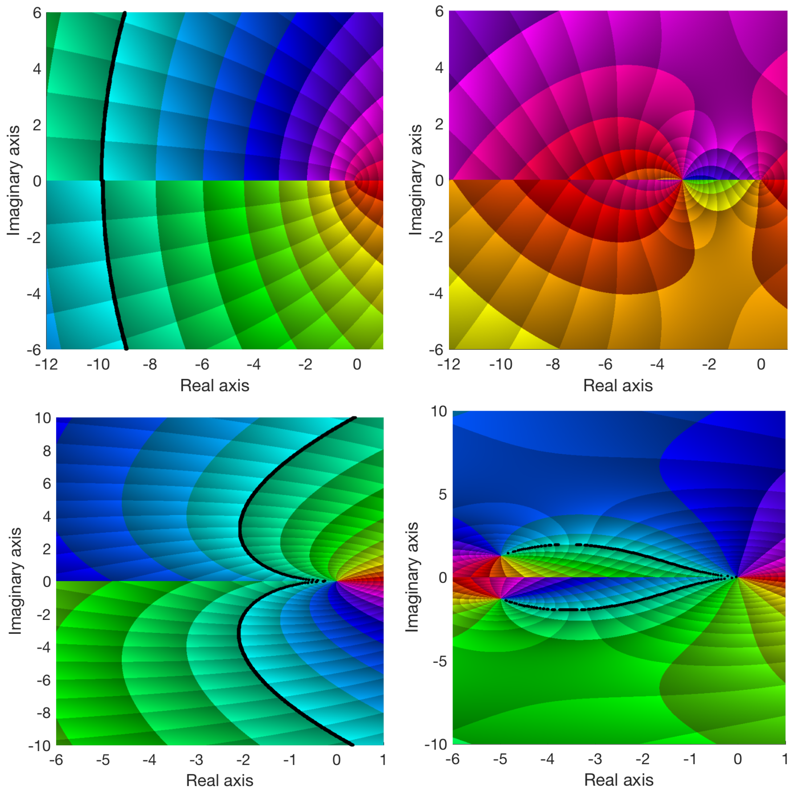
Example 4, Merrikh-Bayat	${\displaystyle \frac{(\sqrt{s}+1)e^{-\sqrt{s}}}{s}}$	$2.67+0.60s^{1.04}+1.08s^{-0.222}$

. The planar projections of the PM diagrams for the systems without and with controller are shown in Figure 4 and Figure 5. The root locus is represented by black dashed lines in the figures. It can be observed that, in all cases, the root locus of the controlled systems contains branches in the stable zone of the complex plane (negative real numbers). It has to be noticed that, for the examples with Riemann surfaces, the PM diagram corresponds to the first Riemann sheet.

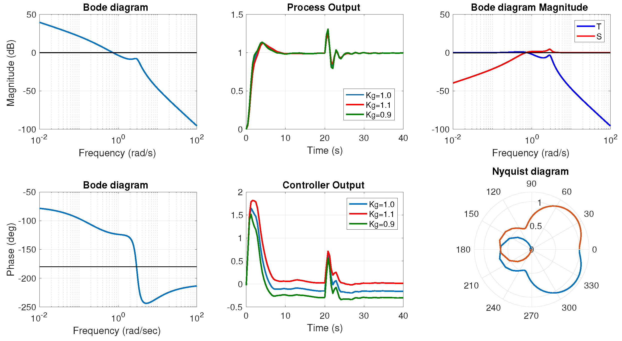
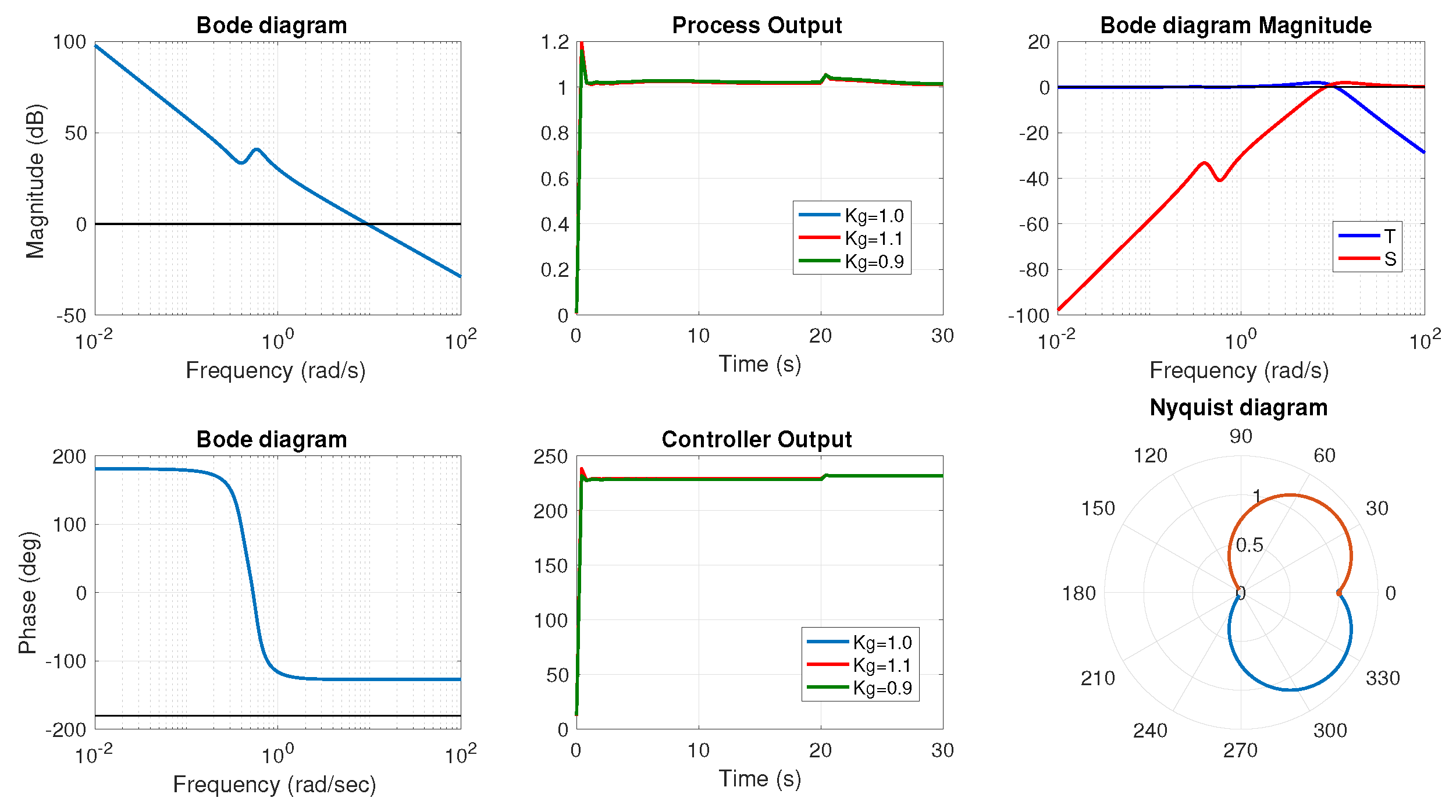
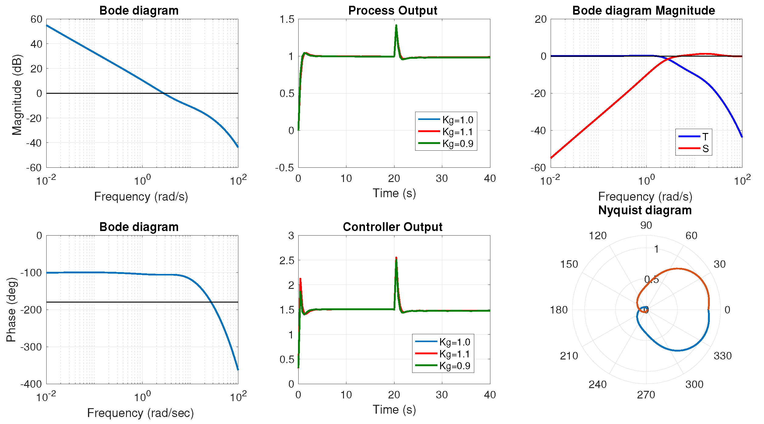
For the controlled systems, the Bode plot, the unit step response, the control action, the high frequency noise rejection, the sensitivity, and the Nyquist plot are represented in Figure 6, Figure 7, Figure 8 and Figure 9. A load disturbance is added when studying the step response. In order to test the robustness to variations in the gain of the plant, the step response when the gain is multiplied by 0.9 and 1.1 is also represented (the multiplication factor is called $K_g$ in the graphs). To examine the behavior of the systems, the parameters of interest that can be extracted from these graphs are represented in

Table 3. Parameters of interest for the examples when controlled. ISE and IAE in squared units and units, respectively, according to the variable that is measured in each example when a unit step is the input. $w_{cg}$ in radians/second. $G_m$ is an absolute magnitude. ${\phi }_m$ in degrees.

	ISE	IAE	${\mathit{w}}_{\mathit{cg}}$	${\mathit{G}}_{\mathit{m}}$	${\mathit{\phi }}_{\mathit{m}}$
Example 1, Podlubny (re-heating furnace)	2.73	4.56	0.8	2.51	57.3
Example 2, Monje (immersed plate)	1.03	2.18	9.3	∞	53.15
Example 3, Aström (heat diffusion)	5.08	14.89	1.8	4.47	142.91
Example 4, Merrikh-Bayat	1.09	1.60	2.8	9.94	74.1

: Integral of the Squared Error (ISE) and Integral of the Absolute Error (IAE), which are generally used performance criteria in stability analysis, crossover frequency ($w_{cg}$), gain margin ($G_m$), and phase margin (${\phi }_m$). The behavior of each system can be studied in detail.

Analyzing the ISE and the IAE, the best values are obtained for the immersed plate and the system proposed by Merrikh-Bayat, respectively. The worst errors are computed when controlling the heat diffusion system because this system presents a steady-state error. The crossover frequency is in the interval given in the specifications. The maximum gain margin is achieved by the immersed plate system. The phase margin is equal to $142.91$ degrees for the heat diffusion system. The minimum value for this parameter is $53.15$ degrees. Observing the graphs, it can be appreciated that the sensitivity at low frequencies and the complementary sensitivity function at high frequencies (noise rejection) present low values that meet the requirements.

Example 1 is described in the book by Podlubny [39]. The author demonstrates that the fractional TF that is given is a more adequate approach to identify the model of a re-heating furnace, but he does not consider how to control this system. In Figure 6, it can be appreciated that the system is robust to changes in the gain of the plant and the behavior when a load disturbance is included is outstanding.

Example 2 represents the model of an immersed plate. The authors have demonstrated that the system is stable. This fact can be easily checked observing the PM diagram. In both cases (with and without controller), the root locus of the system is in the left half plane, which corresponds to negative roots in the characteristic equation. The system maintains the good behavior shown in the previous example (robust to gain changes, load disturbance). The ISE and the IAE present low values, which implies that the final value is reached fast.

Example 3 models the heat propagation in a semi-infinite metal rod. The author did not perform any stability analysis of the system, nor did he propose any controller to regulate the temperature. It can be checked that a fractional order controller can be proposed to efficiently control the temperature. This system presents a steady-state error, which worsens the ISE and the IAE.

In example 4, the stability analysis is not straightforward because this system presents a multi-valued function of s defined on a Riemann surface with a finite number of Riemann sheets where the origin is a branch point. The authors propose a numerical algorithm to find the roots of the characteristic equation on the right-half plane of the first Riemann sheet. After checking the stability, they conclude that the system is stable for values of gain (K in the characteristic equation) lower than $21.51$. In the current approach, the system is not only stable but presents good dynamic properties (overshoot, load disturbance, phase margin), as can be appreciated in Figure 9.

7. Conclusions

This paper presents a simple and intuitive tool that can be applied to model any type of non-rational system if it can be represented by a TF in the s-plane. This tool, called a PM diagram, can be combined with any control method to tune the parameters of a controller that meets the specifications defined for a given system. In this case, a tuning strategy has been applied that optimizes the variables of a fractional order $P{I}^{\lambda }{D}^{\mu }$ controller using an evolutionary optimizer. The fitness function of this filter is defined in the frequency domain. The main requirement is to obtain a flat phase in open loop, which is equivalent to robustness to variations in the gain of the plant. More constraints are also included. The same technique was applied in our previous work with satisfactory results when controlling rational systems.

This tool has many interesting advantages: it simplifies the concepts related to the TF and the non-rational system when computing the parameters of a controller that meets the specifications, and it provides us with a representation of the TF that is complete, easy to obtain, visual, and intuitive. It can also be seen as an adequate technique to be used in education in control courses, especially for non-rational systems where the classical methods are more complex to explain and to understand.

In order to test the proposed strategy, its performance when applied to four different non-rational systems studied by other researchers in this field are examined. In the experiments carried out in this paper, it is proven that our current approach can be used both to model the TF characteristics of these complex non-rational systems and to compute controllers that meet the control requirements for all of them.