Abstract
Obtaining the inverse of a nonlinear monotonic function over a given interval is a common problem in pure and applied mathematics, the most famous example being Kepler’s description of orbital motion in the two-body approximation. In traditional numerical approaches, this problem is reduced to solving the nonlinear equation in each point y of the co-domain. However, modern applications of orbital mechanics for Kepler’s equation, especially in many-body problems, require highly optimized numerical performance. Ongoing efforts continually attempt to improve such performance. Recently, we introduced a novel method for computing the inverse of a one-dimensional function, called the fast switch and spline inversion (FSSI) algorithm. It works by obtaining an accurate interpolation of the inverse function over an entire interval with a very small generation time. Here, we describe two significant improvements with respect to the performance of the original algorithm. First, the indices of the intervals for building the spline are obtained by k-vector search combined with bisection, thereby making the generation time even smaller. Second, in the case of Kepler’s equation, a multistep method for the optimized calculation of the breakpoints of the spline polynomial was designed and implemented in Cython. We demonstrate results that accurately solve Kepler’s equation for any value of the eccentricity , with , which is the limiting error in double precision. Even with modest current hardware, the CPU generation time for obtaining the solution with high accuracy in a large number of points of the co-domain can be kept to around a few nanoseconds per point.
1. Introduction
The inversion of a nonlinear monotonic function is a fundamental mathematical problem that appears in many scientific and technological applications. A famous example is Kepler’s equation [1,2,3], describing bound orbital motion in the two body approximation,
where is the eccentricity; , called the mean anomaly, is a dimensionless quantity—more precisely, an angular measure—of the time t elapsed since periapsis; h and p are the angular momentum per unit mass and the distance at periapsis, respectively (see, e.g., page 151 of reference [3]); and x is the eccentric anomaly, which is related to the angle between the direction of periapsis and the position of the orbiting body at time t (also called the true anomaly) through the equation,
Therefore, obtaining the angular position of an orbiting body for any time is equivalent to computing the inverse of the function in Equation (1), .
In general, a common approach is to solve the equation iteratively for each value of y, using generalizations of the Newton–Raphson algorithm [4,5,6,7,8], or multipoint methods [9,10,11,12,13,14,15,16,17], or a combination of k-vector search with another inversion method, such as Newton–Raphson [18,19,20]. Moreover, special algorithms can be designed for a given function. In the case of Kepler’s equation, several numerical algorithms have been crafted throughout the centuries [1]. Efforts of the last few decades have been focused on developing ever faster computational strategies, mostly based on the Newton–Raphson’s method for the inversion, combined either with a previous analytical stage [21,22], or with the use of pre-computed tables for efficient first guesses [23,24,25], or with CORDIC-like methods for avoiding the evaluation of transcendental functions [26]. As discussed in reference [26], these efforts can be important for tasks that require the solution of Kepler’s equation for a large number of points, such as the search for exoplanets, the modeling of planet formation, or the study of the evolution of star clusters.
Recently, a fast switch and spline inversion (FSSI) scheme has been proposed as an efficient method to compute the values of the inverse of a monotonic function over an entire interval or for a large number of points [27]. This algorithm does not require an initial guess, it is non-iterative, and it solves the equation for all points y at once over a given co-domain . At the algorithm’s core, are the computations of the spline coefficients and breakpoints of the inverse function interpolation. As implemented, it produces a much lower error than that predicted from a naive and direct application of spline theory [27]. Shortly after its first publication in preprint form, the FSSI method [27] was cited and used for high-throughput calculation of many high-eccentricity orbits [28], and considered as a viable high-performance option for accelerating orbital computations of exoplanet modeling [29].
In reference [27], the FSSI scheme was implemented in Python, by using library routines from SciPy [30,31] for the evaluation of the piecewise polynomial in each point y of the co-domain. These library routines use the bisection method [32]—also called the binary search method—for finding the interval between two different breakpoints and of the FSSI spline that contains the evaluation point y such that .
In this work, significant improvements in the FSSI algorithm are described.
The first improvement is the use of a faster search method for finding the interval of j of the FSSI spline to which the evaluation point belongs. The use of a k-vector search for bracketing, followed by the last step of binary search, enables a significant execution time reduction compared to the use of only a bisection method.
Note that both the FSSI and k-vector methods can be used to invert functions in combination with another method. The FSSI, as described in reference [27], requires the use of a search algorithm, while the scheme proposed in references [18,19,20] uses k-vector search followed by a Newton–Raphson inversion. The combination of the FSSI with the k-vector search is quite natural, considering that the setup phases of both methods can be merged. The resulting reduction in generation time can be important, without significantly increasing the pre-processing time cost of either the FSSI or the k-vector algorithms. A further reduction in the execution time can also be obtained when the inverse function is computed for a sorted array Y consisting of a very large number of N elements. In the latter case, the FSSI implementations that use a bisection method with or without a k-vector bracketing become equivalent in terms of generation time. These improvements can be applied to any monotonic function.
For the case of Kepler’s equation, we designed a multistep method that reduces the number of breakpoints used by the FSSI. This reduction is important for values of the eccentricity close to the limit , and allows the FSSI to solve Kepler’s equation accurately for every value of the eccentricity , with being the intrinsic computational error ( in double precision arithmetic). For , the accuracy can be set to , while for it can be as low as for most values of and y. Only for close to the limit , which is also stiff in other methods [33,34,35], is there a small region, , for which the accuracy is found to be limited to ∼.
For the numerical calculations, all the routines have been implemented in Cython [36], a superset of the Python language. This language provides special data types and control-structure semantics for efficient and optimized translation to pure C language with Python bindings (through Python’s C/API function call library). The result of this strategy is that when the Cython code is compiled as a shared-object binary (with the GNU C-compiler gcc), the code executes with the speed of a normal C binary (without the Python interpreter) but can be imported and called from a Python script.
2. Overview of the FSSI Algorithm
Let be an input function that is monotonic over a domain . Hereafter, will also be assumed to be ascending, as in the case of Kepler’s equation. The inversion of a descending function can be computed similarly, with simple changes, or by noting that and applying to the results that will be obtained for an ascending function.
The FSSI algorithm [27] can be used to obtain a piecewise cubic spline interpolation of the inverse function for any y belonging to the co-domain , with and . This algorithm consists of two parts, which will be called “setup” and “generation” procedures, respectively.
2.1. Setup Procedure
When the function and its derivative are known continuous functions, such as the case of Kepler’s problem, the setup procedure of the FSSI algorithm consists of the following basic steps:
- (i)
- Grid generation. A grid of points is generated where , with and . In the examples given in reference [27], these points were chosen to be equally spaced. Here, the step sizes , for , are allowed to be a function of j. The values of are chosen in order to control the error at the desired level over the entire interval, as shown in Section 3.
- (ii)
- Computation of the breakpoints and coefficients. First, the values of the function, , which will provide the breakpoints of the spline interpolation of , and of the derivative of its inverse, , are computed on the grid . This is done given the assumption that over the entire domain. In practice, this demands that should be larger than the numerical error over the interval . When applied to the solution of Kepler’s equation (1), this constraint becomes for every x, or equivalently, . In fact, the multistep version of the FSSI algorithm provides a manner for obtaining the solution of Kepler’s equation even in the limiting case with an accuracy down to ∼.Second, following reference [27], and defining , the coefficients of the spline interpolation of the inverse function in the interval are computed using the equationsfor . These formulas have been derived assuming that none of the differences is zero. Numerically, the expressions for the coefficients and in Equation (3) seem to require not only , but also and for every j. In double precision arithmetic, this would imply that the grid spacing should be controlled to keep . Fortunately, this requirement can be relaxed since , so that the opposite signs in the last two Equation (3) imply thatSince these two coefficients have to be multiplied by and , respectively, with , their contributions to the interpolation of the inverse function, , are expected to be at most of the order . Therefore, and can be set to zero when is smaller than the numerical precision, i.e., when given in double precision arithmetic. These considerations are later used in the numerical implementation of the algorithm.
- (iii)
- Computation of the k-vector. If the generation procedure includes an implementation of the k-vector search algorithm [18,19,20] (as described below), the k-vector should also be computed at the setup stage. As discussed in Section 3, the main part of this computation can be performed during the j loop in point (ii) above. The implementation of the k-vector search in the FSSI algorithm is quite natural since they both use a setup process to minimize their generation time.Since the array y of the breakpoints obtained in point (ii) is given in ascending order, following references [18,19,20] we can define its associated k-vector k as an array of size whose element is given by the maximum index j, such that , for . The constants , m, and q are chosen to be , and . Thus describes a line of equally spaced points such that and , which can be used for a fast interpolation search as discussed below in point (i) of the generation procedure.
These setup computations are executed once for a given function and a given error level, thereby generating the breakpoints and the coefficients of the spline interpolation S of the inverse function , along with the values of the k-vector. These values can be stored as tables of constants either in a file or in the RAM memory. As seen in Section 4 for the Kepler equation, high accuracy can be obtained with only grid points.
2.2. Generation Procedure
The spline breakpoints and coefficients obtained in the setup stage can then be used to evaluate on any set (or array, in computer language) of N points belonging to the interval . The generation procedure to compute the values of on the output array Y consists of the following steps:
- (i)
- Search for the interval. For each point , find the index of the breakpoints such that , with an integer in the range and the possible values of a being . This search can be executed using the bisection method [32], as in the examples of reference [27], or with a different search algorithm, such as the combination of the k-vector search and the bisection method (see Section 3). In the latter case, the k-vector is used for a first bracketing of the possible values of by computing the integer part (floor) and the k-vector values and . Following references [18,19,20], the index is constrained to be in the interval . As discussed in Section 4, a higher accuracy can be obtained with FSSI by selecting a slightly more conservative choice, including one more point in the bracketing, . Finally, a binary search is performed within this reduced interval to obtain the value of the index . This last execution is very fast since it only involves a very small number of points.
- (ii)
- Evaluation. Evaluate the values of for with the formulaThis task only requires a few multiplications and a sum involving numbers that have been computed previously and are given in a table; thus, it is very fast.
2.3. Errors of the FSSI Algorithm
If the function is infinitely differentiable, as for Kepler’s equation, an excellent approximate upper limit for the accuracy of the FSSI algorithm can be given analytically [27].
where , , , and are the derivatives of f of order from 1 to 4, respectively. As said in reference [27], this error is in general several orders of magnitude smaller than that expected from general spline interpolation theory.
Equation (6) can be applied to the error in each interval , so that
This is due to the fact that the FSSI algorithm can be used to invert the function in each grid interval, for which and can be replaced with and , respectively. Once the numerical interpolation of the inverse function is obtained, this prediction for the error can be compared with the numerical error, which can be computed a posteriori by evaluating on the output array Y [27].
One consequence of Equation (7) is that the error of the FSSI algorithm, , scales as the fourth power of the grid interval , which can be thought of as the error of x previous to executing the FSSI spline interpolation. As mentioned above, and shown in Section 4, the spline interpolation provides an average accuracy improvement of more than 10 orders of magnitude, from an average to , with a marginal additional cost in the generation time.
Equation (7) can also be used to optimize the FSSI algorithm by choosing a variable grid spacing . The maximum step size compatible with a given global error level can be obtained by inverting Equation (7) as,
This optimal choice of the grid spacing , entering point 1 in the setup procedure as outlined above, is applied to Kepler’s equation in Section 3.
3. Methods
In this section, the detailed implementation of the FSSI algorithm is discussed, including improvements such as the multistep optimization and the use of the k-vector search. Simple pseudocode listings are provided with array indices following similar conventions to those used in C and Python languages. Most of these routines can be applied to a general monotonic function with minimal or no modifications. An exception is the multistep optimization, which is given specifically for Kepler’s problem, although the procedure described in this case can be adapted to more general monotonic functions.
In the case of Kepler’s problem, the function satisfies the equations , and , for every integer q. This also implies the periodicity equations
for every integer q. Therefore, without any loss of generality, it is sufficient to invert f in the interval , with and , and then the solution for every can be obtained using Equation (9).
For convenience, the eccentricity is considered an input variable to the program, such that the function f and its derivative dfdx are functions of . The eccentricity is denoted ec in the code to distinguish it from Euler’s number. The pseudocode defining Kepler’s functions is shown in Listing 1.

Listing 1.
Pseudocode for defining Kepler’s functions.
Listing 1.
Pseudocode for defining Kepler’s functions.
| function f(ec, x): |
| return x - ec*sin(x) |
| function dfdx(ec, x): |
| return 1. - ec*cos(x) |
3.1. Grid Generation with Multistep Optimization for Kepler’s Equation
In the case of Kepler’s Equation (1), the function f and its derivatives are known analytically, and the expression (8) for the step size compatible with a given error level can be written as
This expression has been obtained from Equation (6), which has been shown to provide a good approximation when is small enough [27]. Therefore, it has to be implemented with a few changes to enforce the validity of this approximation and to avoid divisions by small numbers that may be close to machine precision. A slightly more conservative—i.e., smaller— expression for than the maximum value given in Equation (10) is shown in Listing 2.
Listing 2.
Pseudocode for computing the step size for Kepler’s equation.
Listing 2.
Pseudocode for computing the step size for Kepler’s equation.
| function hstep_kepler(ec, ec2, hgfac, x): |
| cx = cos(x) |
| esx = ec*sin(x) + 2.3e-16 |
| hg = 1.-ec*cx |
| aux = (1. - 15.*ec2 + 6.*ec2*cx*cx + 8.*ec*cx)*hg*esx |
| if aux < 0: |
| aux = - aux |
| aux = aux^0.25 + 2.3e-16 |
| hg = hgfac*hg/aux + 2.3e-16 |
| aux = 0.05/(ec + 0.1) |
| if hg > aux: |
| hg = aux |
| hg = 0.9*hg/(1. + 0.2*ec2) |
| return hg |
The values of ec , ec2, and hgfac shall be passed with the calling of the function, as shown below. The last if statement has been chosen empirically to keep small enough so that the approximations for the error are still valid for every .
Function hstep_kepler, as shown in Listing 2, can be used to generate the array of grid intervals . For a small enough , the minimum value in Equation (10) is obtained in one of the endpoints, or , except in a few intervals. The additional factors that have been introduced in the function hstep_kepler, as compared to Equation (10), have been found to be sufficient to ensure that the choice of the endpoint that minimizes hstep_kepler always gives an error below , if the latter is set at a level ≥, except for equal or very close to and y very close to zero, in which case a limiting accuracy ∼ is found when using double precision arithmetic—see Section 4. Remarkably, this function works for every , thereby including the highly nonlinear regime of eccentricity values close to 1 that is within the computational error in double precision.
The array of grid intervals can then be generated with the pseudocode of Listing 3.
Listing 3.
Pseudocode for generating the grid interval.
Listing 3.
Pseudocode for generating the grid interval.
| x1i = xmin |
| ec2 = ec*ec |
| hgfac = 4.4*((errorlevel)^0.25) |
| hgrid1 = hstep_kepler(ec, ec2, hgfac, x1i) |
| j = 0 |
| while x1i < xmax: |
| hgrid0 = hgrid1 |
| x0i = x1i |
| x1i = x0i + hgrid0 |
| hgrid1 = hstep_kepler(ec, ec2, hgfac, x1i) |
| if hgrid1 < hgrid0: |
| x1i = x0i + hgrid1 |
| h[j] = hgrid1 |
| else: |
| h[j] = hgrid0 |
| j += 1 |
| h[j - 1] = xmax - x0i |
| n = j |
In a computer implementation of the algorithm, the array h can be initialized by dynamic memory allocation, or by assigning a size that is greater than the maximum value of n that may be required for and for error level down to . This value can be chosen to be 26,000, as shall be seen in Section 4. After running the routine hstep_kepler with the while loop shown above, the value of the required number of grid intervals n will be available, along with the values of h[j]. This value of n will be used to allocate the memory for the arrays of the breakpoints, of the coefficients, and the k-vector.
3.2. Computation of the Breakpoints and Coefficients
Pseudocode implementing the formulas given in Section 2 for the computation of the arrays of the breakpoints , called y[j] in the code, and of the coefficients , called c[q,j], is given in Listing 4.
Listing 4.
Pseudocode for computing the breakpoints and coefficients of the spline interpolation of f−1.
Listing 4.
Pseudocode for computing the breakpoints and coefficients of the spline interpolation of f−1.
| function FSSI_coef(xmin, xmax, n, ec, h): |
| y1i = f(ec, xmin) |
| d1i = 1./dfdx(ec, xmin) |
| x1i = xmin |
| for igrid in range(0, n): |
| x0i = x1i |
| hgrid = h[igrid] |
| x1i = x1i + hgrid |
| c[3,igrid] = x0i |
| y0i = y1i |
| y1i = f(ec, x1i) |
| y[igrid] = y0i |
| d0i = d1i |
| c[2,igrid] = d0i |
| d1i = 1./dfdx(ec, x1i) |
| dydh = (y1i - y0i)/hgrid |
| if dydh < 2.22e-16 or hgrid < 1.49e-8: |
| c[1,igrid] = 0. |
| c[0,igrid] = 0. |
| else: |
| c[1,igrid] = ((-(2.*d0i + d1i) + 3./dydh)/hgrid)/dydh |
| c[0,igrid] = (((((d0i + d1i) - 2./dydh)/hgrid)/dydh)/dydh)/hgrid |
| y[n] = y1i |
| return y, c |
As written, the routine FSSI_coef of Listing 4 is applied here to Kepler’s function f(ec, x). However, it can also be used to obtain the breakpoints of more general monotonic functions, if an array of grid steps h and the values of the derivatives are provided.
The arrays y and c have to be initialized by allocating and “double” values, respectively, with the value of n that has been obtained in stage 1 of the setup phase. Then the breakpoints and the coefficients for the spline interpolation of the inverse of Kepler’s function can be obtained with the call,
| y, c = FSSI_coef(0., PI, n, ec, h) |
by providing the number of grid intervals n, the array of grid steps h, and the input eccentricity ec.
3.3. Computation of the k-Vector
When the interval search in the generation procedure is performed using the k-vector method, a pre-processing computation of the k-vector has to be implemented in the setup phase. This can be done within the routine FSSI_coef, using the same for loop to compute the contributions to the k-vector. The pseudocode for computing breakpoints, coefficients of the spline, and k-vector is called with the following routine:
| function FSSI_coef_kv(xmin, xmax, n, ec, h, mkv, qkv): |
This function is based upon the pseudocode FSSI_coef, but with the modifications in the for loop over igrid that are provided in Listing 5.
Listing 5.
Pseudocode for the computation of the k-vector.
Listing 5.
Pseudocode for the computation of the k-vector.
| for igrid in range(0, n): |
| … |
| … |
| c[0,igrid] = (((((d0i + d1i) - 2./dydh)/hgrid)/dydh)/dydh)/hgrid |
| yj = (y0i - qkv)/mkv |
| jy = int(yj) + 1 |
| if jy > 0 and jy < n: |
| deltakv[jy] += 1 |
| kv[n] = n + 1 |
| kv[0] = 0 |
| kvj = 0 |
| for j in range (1, n): |
| kvj = kvj + deltakv[j] |
| kv[j] = kvj |
| y[n] = y1i |
| return y, c, kv |
In Listing 5, the dots … represent the same code as in routine FSSI_coef.
As in the previous case, the arrays y and c must be initialized together with the function FSSI_coef, while the integer arrays kv and deltakv of size are allocated and initialized to zero. Similar to FSSI_coef, this routine can be applied to any function and is not specific to Kepler’s equation as described here.
3.4. Generation Procedure: Search of the Interval
The search of the index corresponding to the interval to which a given point belongs, i.e., , can be executed using the bisection method [32] with the routine described by the pseudocode shown in Listing 6.
Listing 6.
Pseudocode for bisection search.
Listing 6.
Pseudocode for bisection search.
| find_interval_BS(y, ny, yval, left, right): |
| while left < right - 1: |
| mid = (right + left)//2 |
| if x[mid] > xval: |
| right = mid |
| else: |
| left = mid |
| return left |
Here, left and right are two indices that are known to bracket the correct interval, and that have to be defined in the function call of the routine, as shown below. Alternatively, as discussed in Section 2, the search can be performed using the k-vector method followed by a bisection search, as shown in Listing 7.
Listing 7.
Pseudocode for k-vector bracketing followed by a bisection search.
Listing 7.
Pseudocode for k-vector bracketing followed by a bisection search.
| find_interval_kv(y, ny, yval, qkv, mkv, left, right): |
| i1 = int((yval - qkv)/mkv) |
| if i1 < 0: |
| return 0 |
| else if i1 > ny - 2: |
| q = kv[ny - 2] - 1 |
| if q > left: |
| left = q |
| else: |
| q = kv[i1] - 1 |
| if q > left: |
| left = q |
| q = kv[i1+1] + 1 |
| if q < right: |
| right = q |
| left = find_interval_BS(y, ny, yval, left, right) |
When the evaluation array Y is sorted and very large, these two routines, find_interval_BS and find_interval_kv, can be made significantly faster by adding the following line in the beginning of the routine:
| if y[left + 1] > yval: return left |
Indeed, for Y large and sorted, many successive points and fall into the same interval between breakpoints, so that . As such, it is convenient to check this condition, thereby exiting further evaluations in the loop if true. The versions of the routines find_interval_BS and find_interval_kv with this additional conditional check are referred to as find_interval_BS_us and find_interval_kv_us, respectively, where the suffix _us denotes “use sorted”.
3.5. Generation Procedure: Evaluation
Once the correct interval has been found, the value of the inverse function in each of the N points of the array Y (called Yp below) can be performed as shown in Listing 8.
Listing 8.
Pseudocode for evaluating the piecewise polynomial that calls the bisection search.
Listing 8.
Pseudocode for evaluating the piecewise polynomial that calls the bisection search.
| function poly_evaluate_BS(c, y, Yp): |
| ny = len(y) |
| i = 0 |
| yvali = y[0] |
| for ip in range(len(Yp)): |
| yval = Yp[ip] |
| if yval < yvali: |
| i = find_interval_BS(y, ny, yval, 0, i + 1) |
| else: |
| i = find_interval_BS(y, ny, yval, i, ny - 1) |
| yvali = yval |
| ymy0 = yval - y[i] |
| ymy02 = ymy0*ymy0 |
| out[ip] = c[3,i] + c[2,i]*ymy0 + c[1,i]*ymy02 + c[0,i]*ymy0*ymy02 |
| return out |
c and y are the coefficients and breakpoints arrays that have been computed in the setup phase. The if yval < yvali environment makes use of the result of the previous step for a first bracketing, and it works both for sorted and for unsorted Y arrays. Similar pseudocode uses the k-vector routine find_interval_kv for the search. In this case, the values m, q, and the k-vector array have to be passed in the definition of the function,
| function poly_evaluate_kv(c, y, kx, mkx, qkv, Yp): |
The only remaining changes with respect to the routine poly_evaluate_BS will be lines calling find_interval_kv, which will be modified as shown in Listing 9.
Listing 9.
Modification of the pseudocode for evaluating the piecewise polynomial using the k-vector.
Listing 9.
Modification of the pseudocode for evaluating the piecewise polynomial using the k-vector.
| if yval < yvali: |
| i = find_interval_kv(y, ny, kv, mkv, qkv, yval, 0, i + 1) |
| else: |
| i = find_interval_kv(y, ny, kv, mkv, qkv, yval, i, ny - 1) |
Note, this generation part of the code is not specific to function inversion. It provides a general method for cubic spline interpolation when the coefficients and breakpoints are known. If these coefficients and breakpoints are those computed with the setup phase of the FSSI algorithm when applied to a function f, the result is the interpolation of the inverse .
4. Results
All the routines described in Section 2 and Section 3 have been implemented from scratch in Cython [36] using double-precision arithmetic, and have been applied to the solution of Kepler’s equation for different values of the eccentricity .
Briefly, a Cython program resembles a Python program but contains specialized directives, data type syntax, and function commands (that act as wrappers, called decorators). This collection of extra syntax allows the CPython interpreter (together with other standard libraries) to generate a pure C program file that can be compiled with the GNU gcc compiler, thereby producing a shared-object binary file. In all our computer code described here (of Section 2 and Section 3), we wrote highly customized Cython code with explicit type and function referencing that would guarantee optimized compilation results that would produce the lowest function call overhead possible.
Additionally, the translated C file from the Cython code is compiled using appropriate gcc optimization switches that could in principle take advantage of low-level vectorization. The result is a shared-object binary that can be imported into a normal Python script, but when executed, runs as a C binary. As mentioned, on appropriate hardware, further acceleration can be obtained by compiling the Cython code with specialized C libraries such as the Intel vector extension and the Intel Math Kernel library. The numerical results presented below were obtained on a standard laptop computer with modest hardware (a 64 bit Intel i7-8565U CPU 1.8 GHz, with 16 GB memory, and with a Linux Mint operating system with 4.15.0-118 kernel).
Figure 1 shows the interpolation of the solution of Kepler’s equation for three representative values of , namely, , , and , with . The diagonal line represents , corresponding to the solution for , describing a circular orbit. Higher deviations of the solution from this linear regime are observed for increasing values of , corresponding to more severe nonlinearity, a well-known behaviour that is described in textbooks [1,2,3]. For this reason, the multistep method that we have described in Section 3 is most important in the regime , especially for values close to the limit .
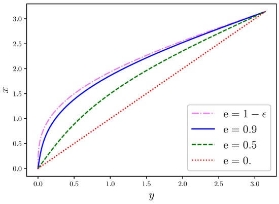
Figure 1.
Solution of Kepler’s equation for different values of the eccentricity ().
Table 1 shows the values of the minimum (fifth column) and maximum (sixth column) step sizes, along with the total number n of steps (fourth column), obtained with the multistep routine for Kepler’s equation that has been described in Section 3. These results are given for four different values of the eccentricity (first column) and five different values of the input error level (second column). For , the actual error (third column), obtained by computing the maximum value of over a large array of y points, is always smaller or at most equal to the input error level because of the conservative assumptions that were made in the design of the routine. For and input accuracy they become equal. For values , and even close to the limit within the numerical error, this multistep routine is able to reach an overall error as small as ∼, which can be reduced to except for values of very close to and for .
Table 1.
Results are shown for the multistep routine with four different values of the eccentricity and input error level. The actual error attained is given along with the number of grid intervals n, and the minimum and maximum steps and that are computed in the setup of the multistep routines. The star * for the actual error in the parenthesis in the limiting case indicates values that apply for . (The errors and the grid intervals are given in radians).
Obtaining higher accuracy, if needed, would require further adjustments or data types higher than double precision.
For , the values of and do not vary by more than a factor 10. In this case, the higher cost in setup time of the multistep routine is not compensated by the reduction of the number of steps, and a single step routine with step size equal to may be preferred, as shown below. However, the multistep routine is very important for , and especially close to the limit , where the ratio can be very large. For and input error level , for example, a single step routine would require steps, while the multitep routine can attain the same precision with just steps. From a practical point of view, we can conclude that the multistep routine is only needed for , and that it is more and more necessary the closer is to 1.
Figure 2 shows the results for the CPU execution time, , of the Cython code corresponding to different variants of the FSSI algorithm, when applied to computing the solution of Kepler’s equation for eccentricity for an increasing number N of points of the co-domain. The input accuracy level is fixed to the value .
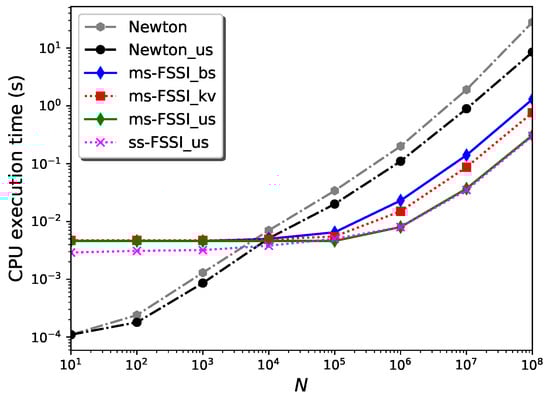
Figure 2.
CPU execution time for different routines as a function of the number N of y values in which the inverse of has to be computed. These results correspond to and an error level . All results have been obtained with the computer hardware specified in the text.
The prefix ms- indicates the routines using the multistep method described in Section 3, as opposed to those indicated with the prefix ss- that use a single step , with 13,500 (for ) to attain the same error level.
The suffixes _bs and _kv label the search routines that are used to find the interval for building the spline in each case, based on the bisection method (_bs), or on the use of k-vector followed by bisection (_kv), respectively. These routines do not exploit the fact the Y array is sorted; it usually is since it is the time variable. However, they can be modified to account for sorted arrays with the addition of the conditional test, if x[left + 1] > xval: return left, as mentioned in Section 3. The resulting _bs_us and _kv_us routines turn out to have the same performance, within the uncertainty; thus, they are indicated with the suffix _us and without the indices _bs and _kv in Figure 2.
For , the CPU execution time is essentially dominated by the setup time. In this regime, for , the single-step routines are faster than the multistep implementations by a factor ∼1.6. In this N regime, and for these values of the eccentricity and error level, the _bs and _kv routines have approximately the same speed.
In the large N regime, the CPU execution time is dominated by the generation time. In this case, the single-step and multistep versions of any of the FSSI routines have the same speed, within a computational error. In this regime, the determining factor of execution time is the search routine. Without the _us enhancement, the FSSI_kv routines using k-vector search followed by bisection are faster than those using bisection, FSSI_bs, by a factor ∼1.6. For sorted Y arrays, however, the _us versions are significantly faster than the "bare" routines _bs and _kv.
For reference, the CPU execution times for a Cython implementation of the Newton–Raphson method—called Newton—are also given in Figure 2. (A similar result, with almost the same values for the execution time, can be obtained with an implementation of Brent’s method [10], which is then not indicated in the figure). Moreover, Newton_us indicates a routine that uses the result of the previous search as a starting guess for each y, resulting in a significant reduction—by a factor ∼3.3 for —of the execution time for large N and sorted Y array, similar to the improvement that has been obtained with the _us variant for the FSSI algorithm. (Such an improvement is not obtained for the Brent method). The routines ms-FSSI_bs_us, ss-FSSI_bs_us, ms-FSSI_kv_us, and FSSI_kv_us are faster by a factor ∼28, for , than the routine Newton_us. Without the _us enhancement, the routines ss-FSSI_kv and ms-FSSI_kv are ∼37 times faster than Newton.
Similar results for the execution time can be obtained for any value of . In this case, the main difference is the comparison between the single-step and the multistep methods, which becomes more and more favorable to the multistep routine for , as discussed previously.
Deeper insight into the performance and the convergence properties of the FSSI algorithm and its variants can be obtained by analyzing how its setup and generation times depend on the accuracy.
Figure 3 shows the dependence of the “setup time,” , on the input error level . This is defined as the part of the CPU execution time that is dedicated to the computation of the spline coefficients and breakpoints and includes the time spent in the multistep routine. In theory, can be expected to be proportional to n, which is proportional to . As shown in the figure, this dependence is satisfied, to a good approximation, for input accuracy below ∼. The deviation from this dependence above this input error level is due to the introduction of the minimum step appearing in the actual multi-step routine, which also implies the—conservative—discrepancy between and the actual error. For this value of , the multistep routine still requires a larger setup time than the single-step routine. As said above and shown in Table 1, this is not the case for higher values of the eccentricity, where the multistep routine becomes more convenient. Finally, Figure 3 shows the small additional CPU-time cost of the setup of the k-vector, as compared with the setup routine that is used together with the bisection method. This additional cost in may be justified when the number of evaluation points N is such that the generation time is higher than the setup time.
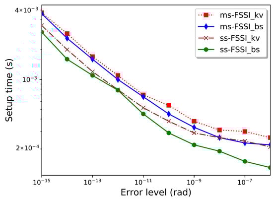
Figure 3.
CPU execution time (s) as a function of the error level for the setup of different routines, as applied to the inversion of with . These results have been obtained with the computer hardware specified in the text.
Finally, Figure 4 shows the dependence of the “generation time” per point of the output array Y, , on the input error level . More precisely, the value given corresponds to for points. Even with the modest hardware, we used in our numerical computations, is just a few nanoseconds per point. Remarkably, for the routines using the k-vector method or the _us enhancement for sorted arrays, turns out to be practically independent of the error level. This is because in these cases the error level is fixed by the setup phase, while the generation phase only requires a few arithmetic operations between numbers that have already been computed in the setup phase, together with a search that, for the _kv and _us methods, only involves a small number of points. In contrast, for the _bs routine, behaves similarly to the bisection method, whose execution time is proportional to [32], which is proportional to . This behavior can be observed in Figure 4 for , the deviations for higher error level being due to the imposition of a maximum value of h in the multistep routine discussed in Section 3.
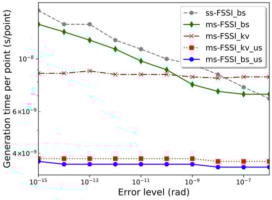
Figure 4.
Generation time per point as a function of the error level for different routines, as applied to the inversion of with . The plotted values correspond to the CPU execution time for generating points, divided by N. These results have been obtained with the computer hardware specified in the text.
5. Discussion
When applied to just a single grid interval, , the FSSI algorithm provides a simple analytical approximation of the inverse function:
whose coefficients can be computed through Equation (3); note that in this case , , , , and . For Kepler’s equation, this gives, , , , , and ; thus,
This approximation can be shown to have an accuracy ∼0.06 rad for , but becomes completely unreliable for . Recently, excellent approximate analytical solutions of Kepler’s equation using a cubic polynomial have been proposed in the literature [37]. The FSSI algorithm, when applied to Kepler’s equation, can be thought of as a generalization of such solutions, using piecewise cubic approximations in suitable sub-intervals.
The FSSI can be convenient for computing the inverse of a monotonic function over an entire interval or a large set of points. If the inversion has to be repeated many times in different sessions, the FSSI method is efficient once the coefficients, the breakpoints, and possibly the k-vector are computed and stored. Then, all subsequent evaluations for obtaining values of the inverse function at each point are very fast, since they would correspond to generation times in the range of a few nanoseconds per point, even with the modest hardware. However, if the values of the inverse function are only required in a reduced number of points, point-by-point methods may be preferred since they can have lower setup times.
A common strategy for accelerating expensive computations of a nonlinear function is to use pre-computed lookup tables (LUT) at evenly distributed intervals and then use interpolation [38,39]. Similarly, the FSSI may constitute a useful tool for creating libraries for inverse functions. Similar libraries could also be created by using other methods, such as Newton–Raphson, by obtaining the inverse in a given grid of points and then extrapolating. However, the FSSI has unique advantages for this purpose, since the values of the inverse function in the n grid points are obtained nearly for free, consisting of just an interchange of and with no generated error, other than the intrinsic computational error . Moreover, the FSSI algorithm, with its choice of the breakpoints and coefficients, has been shown to provide a huge enhancement in precision, as compared to the prediction of error with general spline interpolation [27].
Although the FSSI algorithm, as described in reference [27] and here, has been designed to invert monotonic functions, such as Kepler’s equation, it may be interesting to explore its possible use in more general cases. In this sense, it is interesting to note that the k-vector method has been used for the multi-valued inversion of non-monotonic functions [20] when applied in conjunction with the Newton–Raphson algorithm. It would then be natural to explore the possibility of replacing the latter with the FSSI and applying the methods of reference [20] to the combination of the FSSI and the k-vector search for inverting non-monotonic functions.
6. Conclusions
In contrast to point-by-point methods that solve the equation for each value of y, the FSSI algorithm [27] generates a piecewise polynomial interpolation of the inverse of a monotonic function over an entire interval at once. Here, two significant improvements to this algorithm have been described. First, we introduced the use of a k-vector search for bracketing, followed in the last step by a binary search, for finding the interval of the FSSI spline to which an evaluation point y belongs. Second, in the particular case of Kepler’s equation for orbital motion, we designed a multistep mechanism that significantly reduces the number of breakpoints needed for the interpolation of the inverse function.
For eccentricity , the accuracy of the FSSI can be set to . In this case, a single step routine can be preferred to a multistep method since its setup time can be significantly smaller. However, for , the multistep mechanism becomes ever more efficient. It can solve Kepler’s equation with an error of for most values of the eccentricity and mean anomaly y. Only for close to the limit , where is the intrinsic computational error, is there a small region, , for which the accuracy is found to be limited to ∼2 .
The use of a k-vector search for bracketing followed by bisection for finding the correct interval significantly reduces the generation time, especially when very high accuracy is desired. When the array of y points (i.e., that which contains the inverse function to be evaluated) is large and sorted, the generation time can be reduced considerably more. As this is an important case, we have separate search algorithm routines with this variant denoted _us.
Even with modest computer hardware, the Cython implementations of these versions of the FSSI algorithm efficiently solve Kepler’s equation for a very large number of N of y values with a generation time of the order of a few nanoseconds per point. Remarkably, the generation times of the implementations of the FSSI algorithm using k-vector bracketing, or using the _us variants of the search routines, are practically independent of the error level. Moreover, in the large N regime, these generation times are smaller by more than an order of magnitude than those of point-to-point inversion methods like Newton–Raphson’s or Brent’s.
These results may be of interest, e.g., for the orbital modeling of exoplanets, which requires solving Kepler’s equation for a large number of points [28,29].
Author Contributions
Conceptualization, D.T. and D.N.O.; methodology, D.T. and D.N.O.; software, D.T. and D.N.O.; validation, D.T. and D.N.O.; formal analysis, D.T. and D.N.O.; investigation, D.T. and D.N.O.; resources, D.T. and D.N.O.; data curation, D.T. and D.N.O.; writing–original draft preparation, D.T. and D.N.O.; writing–review and editing, D.T. and D.N.O. All authors have read and agreed to the published version of the manuscript.
Funding
This research was funded by Ministerio de Economia, Industria y Competitividad, Spain, grant number FIS2017-83762-P, and by Conselleria de Educación, Universidade e Formacion Profesional, Xunta de Galicia, grant number ED431B 2018/57.
Acknowledgments
We thank Angel Paredes for discussions.
Conflicts of Interest
The authors declare no conflict of interest.
References
- Colwell, P. Solving Kepler’s Equation Over Three Centuries; Willmann-Bell Inc.: Richmond, VA, USA, 1993. [Google Scholar]
- Prussing, J.E.; Conway, B.A. Orbital Mechanics, 2nd ed.; Oxford University Press: Oxford, UK, 2012. [Google Scholar]
- Curtis, H.D. Orbital Mechanics for Engineering Students, 3rd ed.; Elsevier: Amsterdam, The Netherlands, 2014. [Google Scholar]
- Mathews, J.H.; Fink, K.D. Numerical Methods Using MATLAB, 4th ed.; Pearson: London, UK, 2004. [Google Scholar]
- Gerlach, J. Accelerated convergence in Newton’s method. Siam Rev. 1994, 36, 272–276. [Google Scholar]
- Palacios, M. Kepler equation and accelerated Newton method. J. Comput. Appl. Math. 2002, 138, 335–346. [Google Scholar]
- Abbasbandy, S. Improving Newton–Raphson method for nonlinear equations by modified Adomian decomposition method. Appl. Math. Comput. 2003, 145, 887–893. [Google Scholar] [CrossRef]
- Abbasbandy, S.; Tan, Y.; Liao, S. Newton-homotopy analysis method for nonlinear equations. Appl. Math. Comput. 2007, 188, 1794–1800. [Google Scholar] [CrossRef]
- Ostrowski, A. Solutions of Equations and System of Equations; Academic Press: New York, NY, USA, 1960. [Google Scholar]
- Brent, R.P. Algorithms for Minimization without Derivatives; Prentice-Hall: Englewood Cliffs, NJ, USA, 1973. [Google Scholar]
- Amat, S.; Busquier, S.; Gutierrez, J. Geometric constructions of iterative functions to solve nonlinear equations. J. Comput. Appl. Math. 2003, 157, 197–205. [Google Scholar]
- Neta, B.; Petkovic, M. Construction of optimal order nonlinear solvers using inverse interpolation. Appl. Math. Comput. 2010, 217, 2448–2455. [Google Scholar]
- Zheng, Q.; Li, J.; Huang, F. An optimal steffensen-type family for solving nonlinear equations. Appl. Math. Comput. 2011, 217, 9592–9597. [Google Scholar] [CrossRef]
- Petkovic, M.; Neta, B.; Petkovic, L.; Dzunic, J. Multipoint Methods for Solving Nonlinear Equations; Academic Press, Elsevier: Amsterdam, The Netherlands, 2013. [Google Scholar]
- Kansal, M.; Kanwar, V.; Bhatia, S. New modifications of Hansen–Patrick’s family with optimal fourth and eighth orders of convergence. Appl. Math. Comput. 2015, 269, 507–519. [Google Scholar] [CrossRef]
- Sharma, J.R.; Arora, H. A new family of optimal eighth order methods with dynamics for nonlinear equations. Appl. Math. Comput. 2016, 273, 924–933. [Google Scholar] [CrossRef]
- Sharifi, S.; Salimi, M.; Siegmund, S.; Lotfi, T. A new class of optimal four-point methods with convergence order 16 for solving nonlinear equations. Math. Comput. Simul. 2016, 119, 69–90. [Google Scholar] [CrossRef]
- Mortari, D.; Neta, B. K-vector range searching techniques. Adv. Astronaut. Sci. 2000, 105, 449–464. [Google Scholar]
- Mortari, D.; Rogers, J. A k-vector approach to sampling, interpolation, and approximation. J. Astronaut. Sci. 2013, 60, 686–706. [Google Scholar] [CrossRef]
- Arnas, D.; Mortari, D. Nonlinear function inversion using k-vector. Appl. Math. Comput. 2018, 320, 754–768. [Google Scholar] [CrossRef]
- Boyd, J.P. Rootfinding for a transcendental equation without a first guess: Polynomialization of Kepler’s equation through Chebyshev polynomial equation of the sine. Appl. Numer. Math. 2007, 57, 12–18. [Google Scholar] [CrossRef]
- Raposo-Pulido, V.; Pelaez, J. An efficient code to solve the Kepler equation. Elliptic case. Mon. Not. R. Astron. Soc. 2017, 467, 1702–1713. [Google Scholar] [CrossRef][Green Version]
- Fukushima, T. A method solving Kepler’s equation without transcendental function evaluations. Celest. Mech. Dyn. Astron. 1997, 66, 309–319. [Google Scholar]
- Fukushima, T. Fast procedure solving universal Kepler’s equation. Celest. Mech. Dyn. Astron. 1999, 75, 201–226. [Google Scholar]
- Feinstein, S.A.; McLaughlin, C.A. Dynamic discretization method for solving Kepler’s equation. Celest. Mech. Dyn. Astron. 2006, 96, 49–62. [Google Scholar] [CrossRef]
- Zechmeister, M. CORDIC-like method for solving Kepler’s equation. Astron. Astrophys. 2018, 619, A128. [Google Scholar] [CrossRef]
- Tommasini, D.; Olivieri, D.N. Fast switch and spline scheme for accurate inversion of nonlinear functions: The new first choice solution to Kepler’s equation. Appl. Math. Comput. 2020, 364, 124677. [Google Scholar] [CrossRef]
- Makarov, V.V.; Veras, D. Chaotic rotation and evolution of asteroids and small planets in high-eccentricity orbits around white dwarfs. Astrophys. J. 2019, 886, 127. [Google Scholar] [CrossRef]
- Eastman, J.D.; Rodriguez, J.E.; Agol, E.; Stassun, K.G.; Beatty, T.G.; Vanderburg, A.; Gaudi, S.; Collins, K.A.; Luger, R. Exofastv2: A public, generalized, publication-quality exoplanet modeling code. arXiv 2019, arXiv:1907.09480. [Google Scholar]
- Numpy. Version 1.19. Available online: https://numpy.org/doc/stable/reference/generated/numpy.searchsorted.html (accessed on 1 October 2020).
- SciPy. Version 1.5.3. Available online: https://docs.scipy.org/doc/scipy-1.5.3/reference/generated/scipy.interpolate.PPoly.html (accessed on 1 October 2020).
- Knuth, D. Sorting and searching. In The Art of Computer Programming, 2nd ed.; Addison-Wesley Professional: Boston, MA, USA, 1998. [Google Scholar]
- Conway, B.A. An improved algorithm due to Laguerre for the solution of Kepler’s equation. Celest. Mech. 1986, 39, 199–211. [Google Scholar]
- Charles, E.D.; Tatum, J.B. The convergence of Newton–Raphson iteration with Kepler’s equation. Celest. Mech. Dyn. Astron. 1998, 69, 357–372. [Google Scholar]
- Stumpf, L. Chaotic behaviour in the Newton iterative function associated with Kepler’s equation. Celest. Mech. Dyn. Astron. 1999, 74, 95–109. [Google Scholar]
- Cython. Version 3.0.0. Available online: https://Cython.org/ (accessed on 1 October 2020).
- Lynden-Bell, D. An approximate analytic inversion of Kepler’s equation. Mon. Not. R. Astron. Soc. 2015, 447, 363–365. [Google Scholar]
- Press, W.H.; Teukolsky, S.A.; Vetterling, W.T.; Flannery, B.P. Numerical Recipes: The Art of Scientific Computing, 3rd ed.; Cambridge University Press: Cambridge, UK, 2007. [Google Scholar]
- Pharr, M.; Fernando, R. GPU Gems 2: Programming Techniques for High-Performance Graphics and General-Purpose Computation, Addison-Wesley Professional: Boston, MA, USA, 2005.
Publisher’s Note: MDPI stays neutral with regard to jurisdictional claims in published maps and institutional affiliations. |
© 2020 by the authors. Licensee MDPI, Basel, Switzerland. This article is an open access article distributed under the terms and conditions of the Creative Commons Attribution (CC BY) license (http://creativecommons.org/licenses/by/4.0/).