Automated Maintenance Data Classification Using Recurrent Neural Network: Enhancement by Spotted Hyena-Based Whale Optimization

Abstract

Data classification has been considered extensively in different fields, such as machine learning, artificial intelligence, pattern recognition, and data mining, and the expansion of classification has yielded immense achievements. The automatic classification of maintenance data has been investigated over the past few decades owing to its usefulness in construction and facility management. To utilize automated data classification in the maintenance field, a data classification model is implemented in this study based on the analysis of different mechanical maintenance data. The developed model involves four main steps: (a) data acquisition, (b) feature extraction, (c) feature selection, and (d) classification. During data acquisition, four types of dataset are collected from the benchmark Google datasets. The attributes of each dataset are further processed for classification. Principal component analysis and first-order and second-order statistical features are computed during the feature extraction process. To reduce the dimensions of the features for error-free classification, feature selection was performed. The hybridization of two algorithms, the Whale Optimization Algorithm (WOA) and Spotted Hyena Optimization (SHO), tends to produce a new algorithm—i.e., a Spotted Hyena-based Whale Optimization Algorithm (SH-WOA), which is adopted for performing feature selection. The selected features are subjected to a deep learning algorithm called Recurrent Neural Network (RNN). To enhance the efficiency of conventional RNNs, the number of hidden neurons in an RNN is optimized using the developed SH-WOA. Finally, the efficacy of the proposed model is verified utilizing the entire dataset. Experimental results show that the developed model can effectively solve uncertain data classification, which minimizes the execution time and enhances efficiency.

1. Introduction

In multiple production areas, mechanical appliances include a wide span of industrial equipment and are crucial in building applications. Moreover, mechanical flaws might cause these types of equipment to malfunction or degrade corrupt specific machinery performances, such as production quality, operation safety, and localization [1]. By assuming the difficulty of the present industrial applications, degradation analysis in machinery has become challenging [2,3]. Moreover, the unexpected failures that occur in mechanical tools may involve simple substitutes of cheap bearings, resulting in significant economic and production losses [4]. Hence, highly complex computer-based degradations with evaluation models are crucial for enhancing the accuracy of failure recognition and preventing unexpected accidents.

Several approaches have been introduced for designing panel information in econometric reviews. Moreover, the cross-lagged structural equation method [5] enables typical associations to be analyzed between two variables by a regression of the lagged score of both variables consisting of the random-effects method [6] and the fixed-effects method [7]. The frequentist estimation approaches can be used to improve the changing of information. Moreover, these techniques typically perform worse for small-sized information and hence confine the original methods because they are of low order.

Machine learning (ML) is a branch of artificial intelligence which learns from accessible data and subsequently introduces models for acquiring consistent predictions [8,9]. In particular, ML utilizes statistics because its core concentration is to create an inference from information for enhancing the introduced models through earlier experience and detected patterns [10]. This type of information is generally fed as an input and the respective response variables in ML are termed features and labels, respectively. Moreover, a structural steel frame has mechanical properties that are classified into features, in which its final drift is classified as a label. Several techniques have been introduced in the past few years to be employed in ML [11]. These models can be categorized into two classes: (i) supervised ML and (ii) unsupervised ML. Supervised ML is generally selected under the ML predictive class [8,12,13]. Supervised learning requires a dataset to be divided into unique training and validation subsets. However, in most scenarios the subsystems in a mechanical tool, such as gear and bearing transmission models, are not sufficiently available or complex for visually examining failures continuously because of the large size of machines, environmental limitations, or time-consuming disassemblies [14,15]. Hence, the early prediction, classification, and degradation evaluation of machine tools are challenging in mechanical maintenance [16,17].

The process of grouping data by relevant categories so that they can be used and protected more effectively is called data classification. The method of classification makes it easier to find and retrieve information. This is more important when it comes to risk management, compliance, and data security. An efficient process for data classification is vital because it can help organizations to decide about the level of control necessary to secure the privacy and integrity of their data. The use of data classification allows us to identify data, manage the data better, and employ an appropriate level of security to the data. Several methods have been introduced for data classification. They include defining the types of data that are collected and stored in an organization’s owned or controlled information system. They also include assessing the data’s sensitivity and the effect of the compromise, loss, or misuse of the data.

With the introduction of Industry 4.0 in the manufacturing domain, there is a huge amount of data generated and recorded with the help of sensors. The data recorded from the sensors are raw data, and they need to be processed before being utilized for decision-making. Predictive maintenance is a cog in the wheel of Industry 4.0, and it requires previously stored data collected from a machine or equipment to predict the maintenance before the damage will occur [18]. The collected raw data need to be classified for further processing; therefore, an efficacious method or algorithm is required to classify the obtained data from sensors in a well-organized manner.

The current bio-inspired ML algorithms are implemented for various applications and offer better results [19]. A metaheuristic is a problem-independent, high-level algorithm that offers a collection of guidelines or strategies to create algorithms for heuristic optimization. Meta-heuristic algorithms are highly efficient in seeking an optimal global solution that motivates us to test the efficacy of the proposed algorithm to solve the problem of classification. Metaheuristic algorithms are also called nature-inspired or bio-inspired optimization techniques, as they mimic the inspiration by observing diverse facets of nature. Most of the familiar techniques gained inspiration from Darwin’s theory of evolution, which may be stated as “the population with inheritable characteristics well fit to the environment will endure”. A few such algorithms based on this idea available in the literature are genetic algorithms, differential evolutions, and evolutionary strategies. Swarm intelligence is another type of nature-inspired technique; such algorithms are designed by studying the intelligent behavior of various species such as birds, ants, gray wolfs, bats, and whales, such as foraging, hunting, eating food, and reproduction.

One among the meta-heuristic family is the Spotted Hyena Optimizer (SHO). The main advantages of SHO include its faster convergence rate, its strong global search, being easy to implement, its simplicity, and its accuracy. The optimization algorithms perform effectively in the exploration phase on multimodal functions, acquiring a better convergence speed during the entire iteration. SHO is similar to the Grey Wolf Optimizer (GWO), which can simulate the hunting behavior of spotted hyenas instead of wolves. The simple SHO algorithm approach focuses on the social and hunting behavior of spotted hyenas. The best search agent is mathematically aware of the location of the prey. In accordance with the best search agent, the rest of the search agents make a group of trusted friends, update their own positions, and save the optimal result so as to achieve an optimal global value by successfully avoiding local optima traps. However, as it is stuck in local optima stagnation, SHO often struggles to achieve an optimal value. For preventing such demerits and boosting SHO’s efficacy in terms of exploratory strength, a new Spotted Hyena-based Whale Optimization Algorithm (SH-WOA) is proposed, as randomization exploration leads the search process to a global peak and faster convergence rate by successfully avoiding local optima trapping with a wide range of solutions to achieve a better explorative power. The developed algorithm can produce the optimal centroid by integrating the combination of SHO in the exploration phase of the WOA. In this paper, the hybridization combines two techniques—namely, SHO and WOA—for better results. Hybridization adds a condition to update positions inside the exploitation phase. It is adopted for performing optimal predictive maintenance planning. This hunting method can find a better solution in a shorter time.

Therefore, the main objectives of this study are as follows:

• To address the challenges encountered by the machine learning algorithm for the data classification of mechanical maintenance data effectively and efficiently;
• To establish an automatic classification system using feature extraction and feature selection using different types of mechanical maintenance datasets;
• To develop and implement a hybrid meta-heuristic algorithm for the feature selection and classification of mechanical maintenance data;
• To analyze and validate the performance of the proposed model using diverse performance measures, demonstrating the reliability and effectiveness of the developed model.

The paper is organized as follows. A comprehensive literature review is provided in Section 2. Section 3 specifies the developed architecture for the mechanical maintenance data classification. The different phases to be adopted for data classification in the mechanical maintenance field are shown in Section 4. Moreover, Section 5 describes the feature selection and deep learning for data classification. Section 6 presents the contribution of the proposed SH-WOA for feature selection and classification. The results and discussions are provided in Section 7. Finally, the discussion and conclusions derived from of the study are presented in Section 8.

2. Literature Review

Lei et al. [13] applied the idea of unsupervised feature learning which used artificial intelligence methods for learning features from raw data. Machines were detected by two-stage learning algorithms. Initially, a sparse filtering and unsupervised two-layer neural network (NN) was employed to automatically learn the features from mechanical vibration signals. Furthermore, soft-max regression was used for the classification. The suggested technique was validated with a motor bearing dataset and a locomotive bearing dataset, separately.

Naik and Kiran [20] conducted the mechanical, microstructural, and chemical classification of a specific type of wheat straw. To determine the mechanical properties, uniaxial tension experiments on wheat straws of various gage lengths were performed. Moreover, pH tests and Fourier transform infrared tests were performed to verify the chemical composition and acidity of wheat straw. To determine the gage length of wheat straw, a naïve Bayes (NB) classifier was trained and employed. To predict the ultimate tensile strength of wheat straw, the multivariate linear regression technique was calibrated. By considering the chemical and mechanical properties acquired in the proposed model, wheat straw was utilized in the real world.

Xiong et al. [21] presented a Bayesian nonparametric regression approach for panel information to classify sequential patterns. The suggested model provided a viable and economical technique which permitted both time-independent spatial variables and exogenous variables to be predictors. The suggested model was evaluated by numerical simulation and then evaluated on an econometric public dataset.

The TF (term frequency) and term frequency–inverse document frequency (TF-IDF) methodology of machine learning was implemented for maintenance data classification [22]. Konstantopoulos et al. [23] applied machine learning for material properties classification and prediction. The K-means algorithm was used for data categorization and data analysis. The random forest algorithm and stochastic gradient boosting algorithm were utilized for data classification, and artificial neural networks were implemented for prediction. Machine learning techniques such as the rain forest algorithm, gradient-boosted machine, support vector machine, deep neural network, etc., are applied for various applications such as coal log data [24], diabetic disease data [25], and tool life prediction [26].

Further, Li et al. [27] suggested a deep learning-driven model classify defects and evaluate degradation, and this was then compared with traditional models. It was demonstrated that the deep neural network (DNN) learns much more difficult, nonlinear transformations through several hidden layers that assist in capturing significant differences and obtain discriminative data from industrial information. Many data-driven models, such as the (SVM), deep belief network, k-nearest neighbors (KNN), and backpropagation neural network, have been utilized to verify the effectiveness of deep learning. It has been demonstrated that the suggested model outperformed conventional models in degradation evaluation for mechanical tools.

Siam et al. [28] introduced a machine learning model that is a class of artificial intelligence to develop a strong machine learning-based framework to verify the efficiency in classifying and predicting structural components. A dataset of 97 reinforced masonry shear walls was employed to show the usage of the suggested model. First, the suggested model was used for exploratory data evaluation to identify the effects of geometrical and mechanical wall responses. An unsupervised algorithm was introduced for grouping walls according to their features. Finally, validation and training were performed for upcoming improvements and a supervised learning model was evaluated to categorize the walls and predict their lateral drifts for failure modes.

Chen et al. [29] introduced a novel approach for mechanical tool fault diagnosis based on image quality assessment. First, data acquisition was performed. Next, a leverage image processing approach was introduced to eliminate noise. Subsequently, a convolutional neural network (CNN)-based approach for image classification was employed. Finally, various mechanical equipment images were clustered into various types and defects were detected. The results proved the robustness and effectiveness of the suggested model.

Mahmodi et al. [30] defined the classification and detection of biodiesel from various sources using an electronic nose during the implementation of statistical training-based and mathematical optimization approaches. Data were collected using an electronic nose equipped with eight metal-oxide semiconductor sensors. The evaluation was performed using various approaches, such as linear discriminant analysis (LDA), quadratic discriminant analysis (QDA), and the SVM. The results indicated that the SVM performed well with a high classification ability.

Zhu et al. [31] suggested a CNN that learned features directly from raw data obtained through supersonic combustion analysis. The feature and raw data were obtained to examine the effects of the feature extraction techniques. The outputs showed that the developed CNN can reveal intrinsic features from raw data.

Akyol, and Alatas [32] proposed a Social Impact Theory-based Optimization (SITO). It is a current intelligent optimization algorithm, and it is used to solve the problems of sentiment analysis. It consists of two approaches—namely, shrinkage and helical update. The fitness functions are flexible to optimize adaptive intelligent algorithms. The output of the system is presented to the user using visualization tools.

Agrawal et al. [33] proposed a Quantum Whale Optimization Algorithm (QWOA). It enhances the exploitation power of the classical WOA, and it is used as a variation operator in the quantum bit representation of people in the population and the quantum rotation gate operator. The algorithm for optimization is carried out in two steps. With Euclidean distance, the input feature space is reduced in the first step. The second stage includes a meta-heuristic approach that optimizes the collection of features while improving the value of fitness.

Devaraj et al. [34] proposed a firefly and improved multi-objective particle swarm optimization (FIMPSO) for managing the demands for workload or application requirements by sharing resources between machines, networks, or servers. The outcome of the simulation showed that the proposed FIMPSO model showed an effective performance relative to other existing methods. Gölcük and Ozsoydan [35] introduced the GWO algorithm, which is a recent swarm intelligence-based metaheuristic algorithm. The evolutionary and adaptive inheritance mechanisms employed in the GWO algorithm can operate directly in the binary domain. In this, the noise of the outcomes are not controllable. Liu et al. [36] developed WOA-LFDE (Levy flight and differential evolution) to solve a job shop scheduling problem. The Levy flight strengthens WOA’s global search and iteration convergence capabilities, while the algorithm enhances WOA’s exploitation and local search capabilities and preserves the variety of solutions to avoid local optima. Dhiman and Kumar [37] suggested the MOSHO (multi-objective spotted hyena optimizer). Multiple objectives optimization problems can be solved with it. The roulette wheel system is used to pick appropriate efficient solutions to model the social and hunting behaviors of spotted hyenas. Local optima prevention and gradient-free mechanism are the benefits of these methods, making them applicable to real-world issues. Xin-gang et al. [38] used the Differential Evolution-Crossover Quantum Particle Swarm Optimization (DE-CQPSO) algorithm to solve the problem of environmental economic dispatch. It is based on the rapid convergence of algorithms for the differential evolution and particle diversity of genetic algorithm crossover operators. A parameter adaptive control approach is used to update the crossover probability to achieve better optimization results, and the problem of multi-objective optimization is solved by a penalty factor.

He et al. [39] developed the Firefly Integrated Optimization Algorithm (FIOA). To ensure high-accuracy identification with fewer features, a rating likelihood objection function is utilized. It can subdivide the entire swarm into many sub-swarms automatically, dealing naturally and efficiently with nonlinear, multimodal optimization problems. However, it does not use the best historical individual solution, which prevents possible premature convergence disadvantages. Ranjini and Murugan [40] introduced the Memory-based Hybrid Dragonfly Optimization Algorithm (MHDOA) for solving numerical optimization problems. It is based on the static and dynamic swarming behavior of dragonflies. It lacks internal memory, which can contribute to its early convergence to local optima. Tuba et al. [41] suggested the Brain Storm Optimization Algorithm (BSOA) for feature selection in medical datasets. It also has broad feature sets where many features are associated with others, so decreasing the feature set is important. The usage of computers in medicine improves the accuracy and speeds up data analysis processes. This needs a faster and more accurate system. Orru et al. [42] implemented ML for predicting faults in centrifugal pumps based on data recorded by sensors mounted on the machine. Multilayer Perceptron (MLP) and SVM were applied, and the results revealed that potential faults were successfully predicted and classified by the applied algorithm.

Ghafil and Jarmaia [43] introduced Dynamic Differential Annealed Optimization (DDAO) to solve a broad range of problems of mathematical optimization where the global minimum or maximum is required. Due to their performance, reliability, and relatively low computation time, metaheuristics have been developed and widely used in various disciplines. More iterations and time are required to reach a location near the global point in the search space. Mahjoubi and Bao [44] framed a hypotrochoid spiral optimization algorithm with a groundbreaking bi-objective function and new variables in order to solve the optimal sensor placement of tri-axial accelerometers for a high-rise construction. It uses a limited number of sensors to obtain much information about a structure. It is difficult to obtain global or near-global optima.

Although many approaches are available for classifying mechanical data, several challenges exist in the existing methodologies; therefore, a new method must be implemented to categorize data based on their problems. Among them, the DNN [27] is used to analyze the degradation of load imbalance and exhibits a good performance. However, a significant amount of data is required to train it. The NB [20] is utilized to determine the gage length and is highly accurate. However, it poses data scarcity. Machine learning efficiently solves critical issues and has been employed for classification and prediction [28]. However, it is a time-consuming method. The CNN is strong and efficient, exhibits a better classification accuracy, afford the best generalization performance, and is stable [31]. However, it is computationally expensive and must be optimized by adjusting the network configuration. The Bayesian nonparametric regression approach is flexible and highly accurate [21]. However, the performance must be improved. Unsupervised two-layer NNs are highly accurate and increase the number of unlabeled data [13]. However, it must learn the weights of NNs. The SVM has high discrimination and classification precision, and it operates based on the linear classification of data [30]. Hence, the challenges specified above should be addressed for better mechanical data classification.

Table 1. Features and challenges of some existing data classification research.

Author	Methodology	Features	Challenges
Li et al. [27]	DNN	It is used to analyze the degradation of load imbalance. Has a better performance.	A significant amount of training data is required.
Naik and Kiran [20]	NB	It is utilized to determine the gage length. It offers a high accuracy.	It poses data scarcity issues.
Siam et al. [28]	Machine Learning	It efficiently solves critical issues. It is employed for classification and prediction.	It is time-consuming.
Chen et al. [29]	CNN	It is strong and efficient. It offers a high stability.	It is computationally expensive.
Xiong et al. [21]	Bayesian nonparametric regression approach	It is flexible. It offers a high accuracy.	Its performance must be improved.
Lei et al. [13]	Unsupervised two-layer NN	It offers a high diagnosis accuracy. It increases the amount of un-labelled information.	The weights of NNs must be learned.
Mahmodi et al. [30]	SVM	Its discrimination and classification precision is high. It performs based on the linear classification of data.	Multiple key parameters must be set correctly to attain the best results.
Zhu et al. [31]	CNN	It offers a good classification accuracy. It offers the best generalization performance.	It has to be optimized by adjusting the network configuration.
Akyol, and Alatas [32]	SITO	It is easy to solve effective and large problems. It is compatible with other modules.	It needs to be updated continuously.
Agrawal et al. [33]	QWOA	It is easy to run with parallel computation. Has a higher probability and efficiency in finding the global optima. It can be efficient for solving problems.	It is challenging to define the preliminary design parameters. It cannot work out the issues of scattering.

shows the features and challenges of some of existing data classification research.

In addition,

Table 2. Features and challenges of some existing metaheuristic algorithms.

Author	Methodology	Features	Challenges
Devaraj et al. [34]	FIMPSO	The speed of convergence is very high in the probability of finding the global optimum.	It has some problems with initializing the design parameters.
Golcuk and Ozsoydan [35]	GWO	It is efficient for local searches. Simple and flexible.	Higher computational cost. No guarantee of global optimality.
Liu et al. [36]	WOA-LFDE	It can increase the population diversity.	Unbalanced exploration and exploitation.
Dhiman and Kumar [37]	MOSHO	Requires less time. High accuracy rate.	Needs further improvement in overhead and detection time.
Xin-gang et al. [38]	DE-CQPSO	It is very efficient in global search algorithm. Simple to implement. Less parameter tuning required.	Needs memory to update velocity. Slow convergence.
He et al. [39]	FIOA	The speed of convergence is very high in the probability of finding the global optimizer.	It does not require a good initial solution to start its process.
Ranjini and Murugan [40]	MHDOA	High accuracy. Increasing population diversity. Strong robustness.	The speed of convergence is slow. Time consuming.
Tuba et al. [41]	BSOA	Improved accuracy. Minimal false point samples.	It is much harder and time-consuming. It is not suitable for large data sets.
Ghafil, and Jarmaia [43]	DDAO	Consumes less energy. Less delay.	The specificity is very low.
Mahjoubi, and Bao [44]	Hypotrochoid spiral optimization algorithm	It provides fast learning capabilities, has a highly generalized performance, and has free parameter tuning.	Enhancement is needed in the machine learning approach. Needs a lot of training data.

shows the features and challenges of an existing meta-heuristic algorithm that should be taken into consideration when introducing a new algorithm with a high performance.

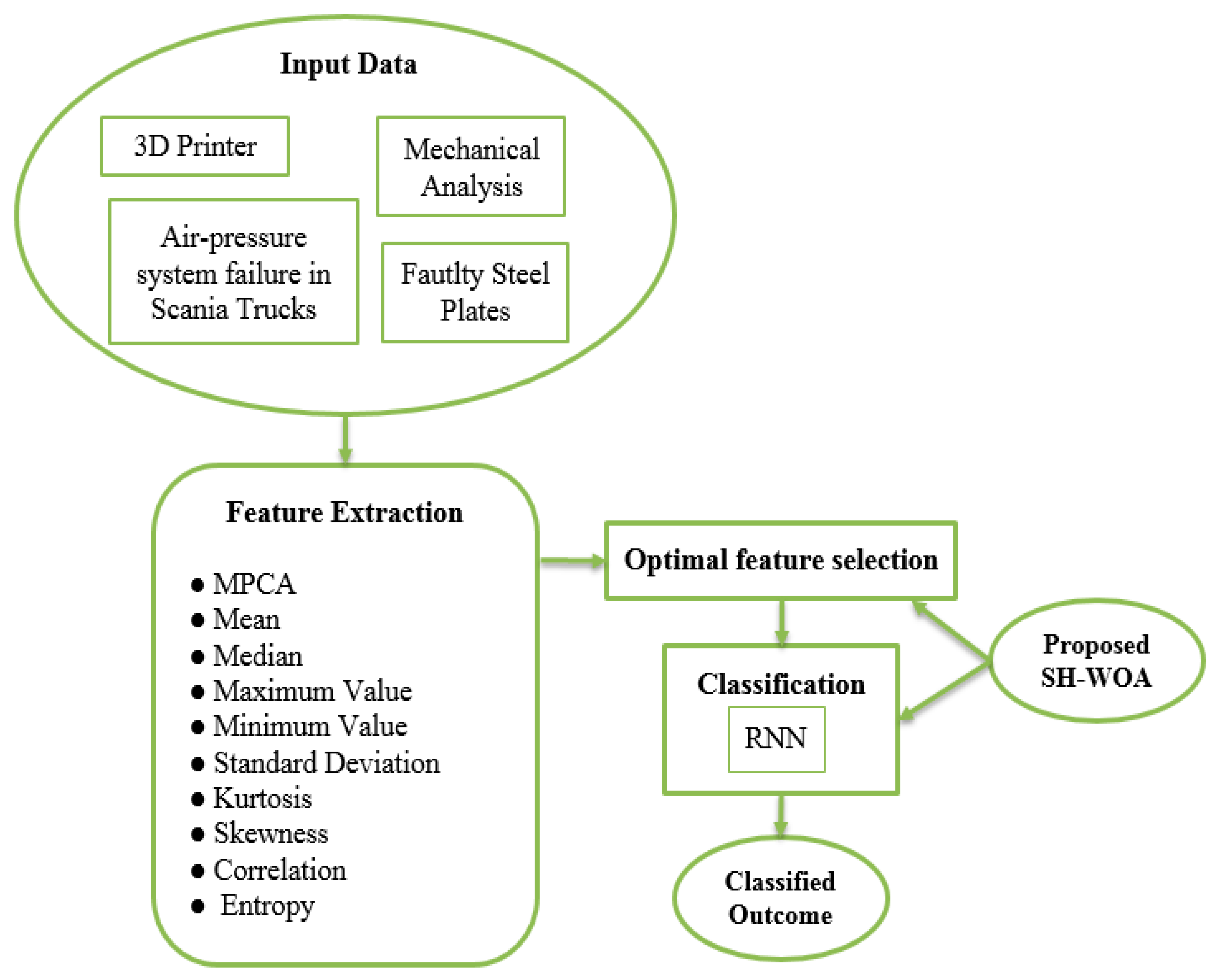
3. Developed Architecture for Mechanical Maintenance Data Classification

In this section, the architecture for data classification is explained.

3.1. Proposed Architecture

In data research, the term big data analytics is defined as “the process of analyzing and understanding the characteristics of massive size datasets by extracting useful geometric and statistical patterns” [45]. Different applications of big data have emerged in the past few years; hence, researchers from multiple disciplines have become cognizant of the beneficial aspects of information or main data extraction from various issues. However, the existing learning techniques cannot be directly applied owing to scalability issues. Hence, deep learning architecture was adopted in the proposed data classification model. Moreover, the proposed model uses four mechanical datasets for efficient and reliable data classification which were obtained from Google datasets. Those datasets were “three-dimensional (3D) printer”, “air pressure system failure in Scania trucks”, “faulty steel plates”, and “mechanical analysis data”. The architectural representation of the proposed mechanical data classification model is shown in Figure 1.

From the datasets, features such as principal component analysis (PCA); first-order statistics such as the mean, median, maximum value, minimum value, and standard deviation; and second-order statistics such as the kurtosis, skewness, correlation, and entropy were extracted. Owing to the higher number of features, a feature selection was performed. The feature selection was performed using the proposed SH-WOA. Moreover, the extracted features were subjected to a classifier—i.e., the recurrent neural network (RNN). To enhance the performance of the traditional classifier, the number of hidden neurons in the RNN was optimized using the proposed SH-WOA algorithm. The main objective of the proposed big data analytics model is to perform feature selection and classification to obtain the maximum classification accuracy.

3.2. Objective Model

As mentioned previously, the proposed mechanical classification model optimizes the features to be selected and the number of hidden neurons in the RNN using the proposed SH-WOA to maximize the classification accuracy. The mathematical formulation for accuracy is represented in Equation (1), in which the variables p, q, r, and s specify the true positive, true negative, false positive, and false negative elements, respectively, during classification.

$$obj= \frac{p+q}{p+q+r+s}.$$

(1)

This objective was attained using the proposed SH-WOA for handling the feature selection and optimized RNN-based classification in the proposed mechanical maintenance data classification model.

4. Different Phases to Be Adopted for Data Classification in Mechanical Maintenance Field

In this section, various steps involved in data classification are explained.

4.1. Data Acquisition

The proposed model utilizes four datasets, as mentioned previously, for the experiments. The description of each dataset is provided below.

3D printer: This dataset evaluates new 3D-printing-related models and its application requires the test information of inputs encountered [46]. A standard dataset must not be obtained from a similar distribution of printed shape in terms of class, representation type, and complexity. A new dataset of 10,000 methods obtained from an online 3D-printing method sharing dataset was introduced using both contextual and geometric characteristics analyses. Subsequently, the demonstration of the dataset revealed more brief explanations of real-world methods employed for 3D-printing over classical datasets. Furthermore, an online query interface was developed to select the subsets of the dataset for project-specific features. The dataset and per-model statistical information are publicly accessible.

Air pressure system failure in Scania trucks: This dataset includes the data gathered from certain Scania trucks daily [47]. The model is focused on an air pressure system (APS) that produces pressurized air, which is used in different functions in a truck—e.g., gear and braking changes. The dataset’s positive class includes the failures of the parts to a particular module of the APS model, whereas the negative class includes the failures of trucks for parts not related to the APS. Moreover, the data comprises the subset of all accessible information selected by specialists.

Faulty steel plates: This dataset is based on research performed by Semeion [48], which is a research center of sciences of communication. The main objective of the research was to accurately categorize the surface fault types in stainless steel plates by six types of possible faults. The input vector comprised 27 indicators, which describe the geometric shape of the fault and its outline. Accordingly, Semeion was commissioned by Centro Sviluppo Materiali to perform the above-mentioned task; hence, details regarding the characteristics of the 27 indicators utilized as i-vectors or the types of the six fault classes cannot be divulged.

Mechanical analysis pumps dataset: This dataset was provided by the University of California ML repository [49]. Every instance comprised several components, each of which contained eight attributes. Various instances in this dataset have a distinct number of components. Moreover, one instance cannot be maintained on one line.

4.2. Feature Extraction

In this context, three feature extraction sets were considered: (1) PCA, (2) first-order statistics, and (3) second-order statistics. First-order features such as the mean, median, maximum value, minimum value, and standard deviation and second-order statistics such as the kurtosis, skewness, correlation, and entropy features were extracted.

1. PCA: It is used to decrease the dimensionality of a dataset by including more interrelated variables and preserving the differences present in the dataset simultaneously [50]. The process of PCA is shown below.

(a) Assume a dataset, B_a, where a = 1, 2, ……, A is the training sample, and each dataset comprises x rows and y columns. The mean value of the training samples, $B_x= \frac{1}{A} {\displaystyle \sum }_{b=1}^A{B}_b, B_a=B_a- B_x,$ was calculated to ensure that the complete mean value of the datasets was equivalent to zero.

(b) The 2D-PCA method was used to compute the feature vectors by all the centralized samples. Therefore, complete feature vectors were standardized to ensure that the norm of each feature vector was equivalent to one. The eigenvectors similar to the vast w eigenvalues of the covariance matrix were the basis of the feature subspace.

(c) All the centralized samples were projected into the subspace; therefore, each dataset representation in the subspace was acquired, and each was denoted as a matrix, including x rows and w columns.

(d) To analyze the sample_, B_tst = B_tst − B_x was considered and B_tst was projected into the subspace. In this case, the matrix was acquired, which included x rows and w columns.

(e) Moreover, independent component analysis (ICA) was conducted for all the feature vectors. Next, a unifix matrix U might be obtained. Hence, a coefficient matrix can be acquired for any dataset present in the sub-space.

(f) The similarity was calculated for any of the two coefficient matrices, $C^1=\left[c_1^1{c}_2^1\cdots c_w^1\right]$ and $C^2=\left[c_1^2{c}_2^2\cdots c_w^2\right]$, using Equation (2):

$$Similarity={\displaystyle \sum _{b=1}^A\frac{c_b^1\times c_b^2}{\Vert c_b^1\Vert \Vert c_b^2\Vert }}.$$

(2)

2. First-order statistics: Five computing features existed in the first-order statistics as follows.

Mean: It can be calculated by summing up and dividing all the numbers in the dataset by the total number in the dataset [19]. The numerical formula of the arithmetic mean is represented by $\overline{m}$, as shown in Equation (3).

$$\overline{m}=\frac{1}{n}{\displaystyle \sum }_{z=1}^n{m}_z.$$

(3)

In Equation (3), the number of values existing in the dataset is denoted as n, the sum of all the numbers is denoted by ∑m_z, and the data are indicated by m_z.

Median: It is used to calculate the average, meaning the middle number, of a set of numbers [19]. If, in the dataset, there are odd numbers of values, then the median value is defined as in Equation (4).

$$Med=size of {\left(\frac{n+1}{2}\right)}^{th}.$$

(4)

If, in the dataset, there are even numbers of values, then the median value is as shown in Equation (5).

$$Med=average of {\left(\frac{n}{2}\right)}^{th},\mathrm{and}{\left(\frac{n+2}{2}\right)}^{th}.$$

(5)

Maximum value: It is the maximum value among all the data points, as expressed in Equation (6).

$$Maxvalue=Max\left(m_z\right).$$

(6)

Minimum value: It is the minimum value among all the data points, as expressed in Equation (7).

$$Minvalue=Min\left(m_z\right).$$

(7)

Standard deviation: It calculates the dispersion of a dataset that corresponds to its mean and measured variance square root [19]. This is denoted by “σ”, where m_z is the individual value present in the given dataset, as represented in Equation (8).

$$\sigma = \frac{1}{n} {{\displaystyle \sum }}_{z=1}^n{\left(m_z-\overline{m}\right)}^2.$$

(8)

3. Higher-order statistics: Four determining features exist in higher-order statistics, as follows:

Kurtosis: It is a statistical measure used for a distribution to be clarified. Inside a tail, it tests extreme values. High kurtosis distributions show tail data exceeding the tails of a normal distribution. Less kurtosis distributions display tail data that is usually less than the tails of a normal distribution [19]. The mathematical equation for kurtosis is given in Equation (9).

Here, $m_4=\frac{\sum {\left(m_z-\overline{m}\right)}^4}{n}$ and $m_2=\frac{\sum {\left(m_z-\overline{m}\right)}^2}{n}$; m₄ is the fourth moment and m₂ is the variance (σ).

$$k{u}_4= \frac{m_4}{m_2^2}.$$

(9)

Skewness: It is the degree of distortion in a collection of data from a normal distribution. It can be positive, negative, zero, or undefined. It is represented in Equation (10), where $m_3=\frac{\sum {\left(m_z-\overline{m}\right)}^3}{n}$ and $m_2=\frac{\sum {\left(m_z-\overline{m}\right)}^2}{n}$; m₂ is the third-moment dataset.

$$s{k}_1= \frac{m_3}{m_2^{\frac{3}{2}}}.$$

(10)

Correlation: It is a statistical indicator of the interaction between two factors. It is finely used in factors which determine the relationship with each other [19]. The computational formula is shown in Equation (11).

$$Co{r}_{ml}= \frac{\sum \left(m_z-\overline{m}\right)\left(l_z-\overline{l}\right)}{\sqrt{\sum {\left(m_z-\overline{m}\right)}^2\sum {\left(l_z-\overline{l}\right)}^2}}.$$

(11)

In the equation above, the term m_z represents the values of the variable m in a sample, $\overline{m}$ denotes the mean values of the variable m, l_z represents the values of the variable l in a sample, and $\overline{l}$ denotes the mean values of the variable l.

Entropy: It is a statistical measure of uncertainty which provides a good measure of intraset distribution when a set of patterns is provided. The numerical formula is denoted in Equation (12), where PR_s is the probability value of obtaining the z^th value.

$$Entropy= -{{\displaystyle \sum }}_{s=1}^{n}P{R}_s{\log }_{2}P{R}_s.$$

(12)

Hence, the combination of the entire set of features with principal component analysis (PCA), first-order statistics, and second-order statistics is represented as a feature vector, as shown in Equation (13).

$$F{r}_k= F{r}_1,F{r}_2, \dots \mathrm{..} , F{r}_{N_{Fr}}.$$

(13)

In Equation (13), k = 1, 2, ……, N_Fr, and N_Fr represents the number of all features extracted.

5. Feature Selection and Deep Learning for Data Classification

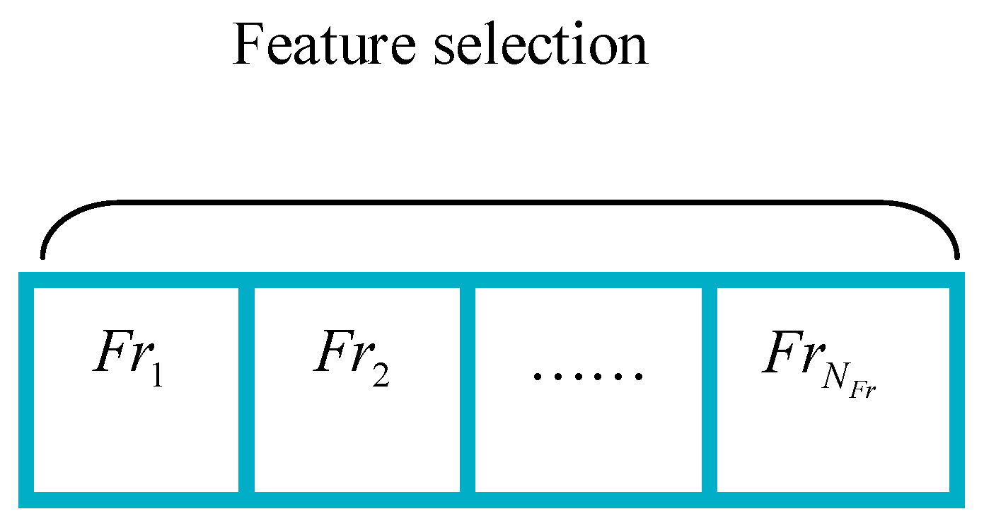
5.1. Feature Selection

As the extracted features are long, a feature selection must be performed. In the proposed mechanical maintenance data classification model, the selection of features is performed using the proposed SH-WOA. After the feature selection, the features are represented based on Equation (14).

$$F{r}_{k\ast }= F{r}_{1\ast },F{r}_{2\ast }, \dots \mathrm{..} , F{r}_{N_{Fr\ast }}.$$

(14)

Here, Fr_k* refers to the selected features and N_Fr* refers to the total number of selected features.

5.2. RNN-Based Classification

The RNN is a type of NN that generates a direct graph by a data sequence [51]. Moreover, it can function with time series information effectively; hence, the result appears to be best while the present and earlier information are determined. Long short-term memory is a new type of RNN that is used for resolving the gradient mass and explosions. Moreover, it generally comprises three gate units—i.e., input, output, and forget gates—as well as memory cell units. Using these three gates, it can eliminate unnecessary data and extract significant related data. To further improve the performance of the RNN, a gated recurrent unit (GRU) is used with the RNN. This GRU combines the “forget and output gates” into a unique update gate up_d, where linear interpolation is performed to obtain the results. Assume e_d ← Fr_k* as the d^th input feature, and H_d-1 denotes the previous hidden state. Equation (15) denotes the result of the update gate up_d, while Equation (16) represents the reset gate rs_d.

$$u{p}_d=acv\left(W{F}^{eup}{e}_d+W{F}^{Hup}{H}_{d-1}\right),$$

(15)

$$r{s}_d=acv\left(W{F}^{ers}{e}_d+W{F}^{Hrs}{H}_{d-1}\right).$$

(16)

In the equation above, the activation function is denoted by acv, which is a logistic sigmoid function in general. The weight function is denoted by WF^d = {WF^eup, WF^Hup, WF^ers, WF^Hrs}, which has to be tuned appropriately by the training algorithm to minimize the error difference between the predicted and original outputs. Moreover, the candidate state of the hidden unit is expressed as in Equation (17).

$${\tilde{H}}_d=\tan \left(W{F}^{eH}{e}_d+W{F}^{HH}\left(H_{d-1}\otimes r{s}_d\right)\right).$$

(17)

In the equation above, element-wise multiplication is denoted as ⊗. The linear interpolation among candidate state $\widetilde{H_d}$ and H_d-1 as well as the d^th-term hidden activation function is denoted as the H_d of the GRU, as shown in Equation (18).

$$H_d=\left(1-u{p}_d\right)\otimes {\tilde{H}}_d+u{p}_d\otimes H_{d-1}{H}_d=\left(1-u{p}_d\right)\otimes {\tilde{H}}_d+u{p}_d\otimes H_{d-1}.$$

(18)

As an improvement to the conventional RNN, the optimized RNN in the proposed model optimizes the number of hidden neurons by the SH-WOA to maximize the classification accuracy.

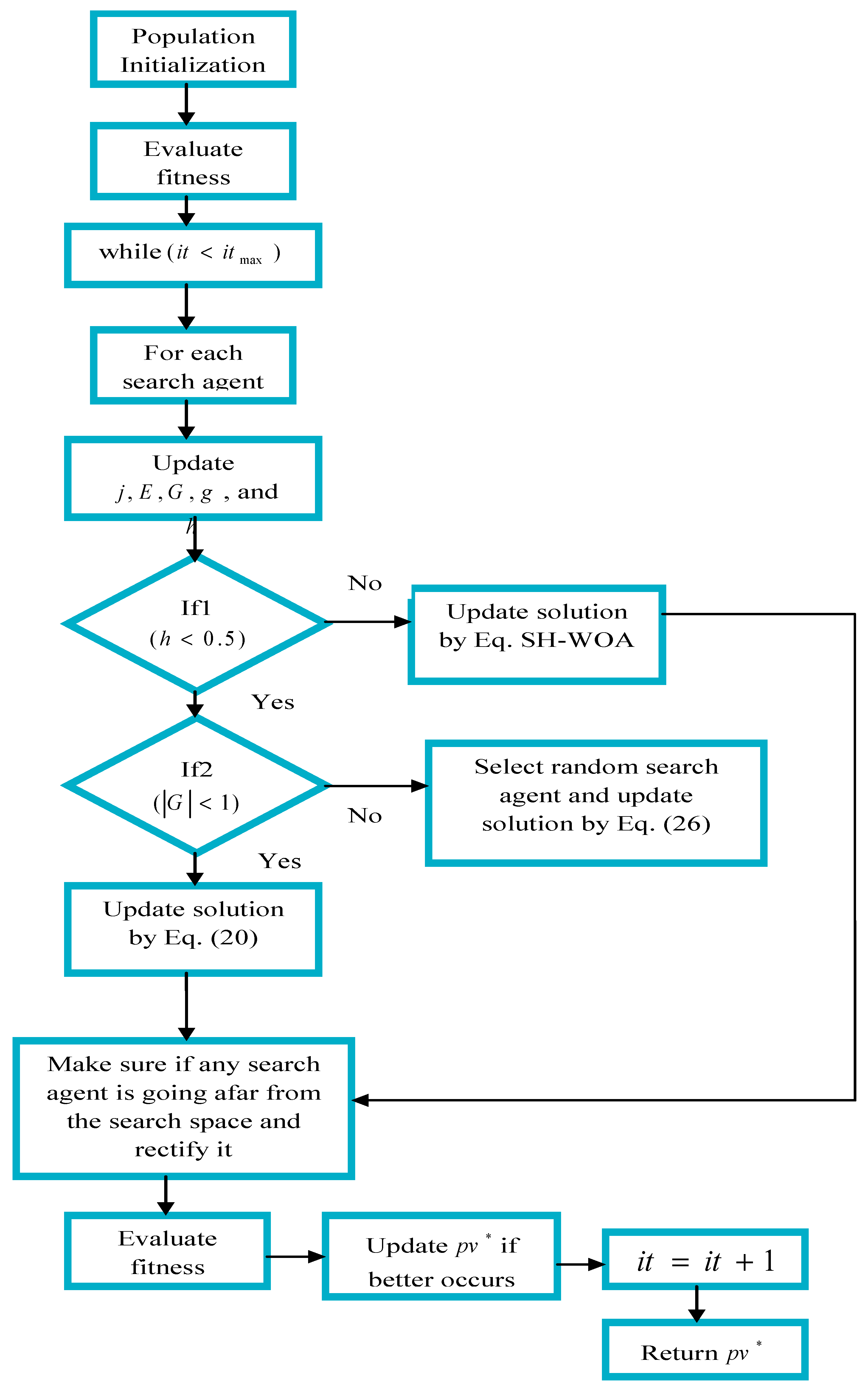
6. Proposed Spotted Hyena-Based Whale Optimization Algorithm for Optimal Feature Selection and Classification

6.1. Flow Diagram of Feature Selection and Classification

The flow diagram of the feature selection and classification is shown in Figure 2. Here, the developed SH-WOA is used to enhance the performance of the proposed mechanical data classification model. The trial and error method has been employed in this work to tune the parameters and is a primitive technique of problem solving. It is characterized by frequent, diverse attempts which persist until success is achieved.

6.2. Solution Encoding

The proposed SH-WOA is adopted for both feature selection and classification. Figure 3 shows a diagrammatic representation of the solution encoding for feature selection and classification.

In Figure 3, Fr_k refers to the features to be selected, from which features such as Fr_k* are obtained. The minimum and maximum bounding limits of the features are 0 and 1, of which 0 indicates the features that are not selected and the selected features are represented by 1. Moreover, the minimum and maximum bounding limits in the RNN-based classification are 5 and 35, respectively.

6.3. Conventional Whale Optimization Algorithm

The traditional WOA [52] is inspired by the hunting mechanism of humpback whales, which are the largest whales of the Baleen whale family. An interesting characteristic of humpback whales is their specific hunting mechanism. These whales can recognize prey and encircle them. Equations (19) and (20) express the encircling behavior.

$$D=\left|E.p{v}^{\ast }\left(it\right)-pv\left(it\right)\right|,$$

(19)

$$pv\left(it+1\right)=p{v}^{\ast }\left(it\right)-G.D.$$

(20)

In the equations above, the coefficient vectors are denoted as $E$ and $G$, the current iteration is denoted as $it$, and the position vector of the acquired best outcome is denoted as $p{v}^{\ast }$. The position vector is denoted by $pv$, the absolute value by $\left|\right|$, and the element-by-element multiplication by “.”. The coefficient vectors are represented by Equations (21) and (22), respectively.

$$E=2.rnv,$$

(21)

$$G=2j.rnv -j.$$

(22)

In Equations (21) and (22), the random vector between 0 and 1 is denoted by $rnv$; furthermore, the term $j$ decreases from 2 to 0 during the entire iteration. To mathematically denote the bubble net method of humpback whales, two approaches can be used: the shrinking encircling and spiral updating position methods. In the former method, the term $j$ is reduced, as shown in Equation (23). In the latter method, the distance between the whale’s position $\left(X,Y\right)$ and the prey’s position $\left(X^{\ast },Y^{\ast }\right)$ is analyzed. Hence, the spiral equation is defined between the whale and prey’s position for impersonating a helix-shaped group of humpback whales, as expressed in Equation (23).

$$pv\left(it+1\right)=D^{\prime }.e^{og}.\cos (2\pi g)+p{v}^{\ast }\left(it\right).$$

(23)

In Equation (23), the term $D=\left|E.p{v}^{\ast }\left(it\right)-pv\left(it\right)\right|$ indicates the distance between a whale and prey, in which the random number ranges from −1 to 1 and is denoted as $g$, and the constant term is denoted as o. To update the solution based on the shrinking encircling mechanism, a mathematical equation is established, as shown in Equation (24).

$$pv\left(it+1\right)=\{\begin{array}{cc}p{v}^{\ast }\left(it\right)-G.D& if h<0.5\\ D^{\prime }.e^{og}.\cos (2\pi g)+p{v}^{\ast }\left(it\right)& if h\ge 0.5\end{array}.$$

(24)

In this equation, the random number h ranges from 0 to 1. Moreover, the position vector pv is used to search the prey vector. The position vector contains random values between −1 and 1, such that the search agent avoids the reference whale. The mathematical formula is expressed in Equations (25) and (26). Here, the random position vector considered from the previous solutions is denoted as pv_rand.

$$D=\left|E.p{v}_{rand}-pv\right|,$$

(25)

$$pv\left(it+1\right)=p{v}_{rand}-G.D.$$

(26)

The pseudocode of the traditional WOA is shown in Algorithm 1.

Algorithm 1. Pseudo code of Conventional Whale Optimization Algorithm [52].
1:	Conduct the population initialization as $p{v}_i$, where $i=1,2,\cdots ,ne$.
2:	Evaluate the fitness value of every search agent.
3:	pv* is the best search agent.
4:	itmax indicates maximum number of iterations.
5:	while (it < itmax)
6:	for each search agent
7:	Update J, E, G, g, and h
8:	if1 (h < 0.5)
9:	if2 (|G| < 1)
10:	Update the solution using Equation (20).
11:	else if2 (|G| ≥ 1)
12:	Select a random agent (pvrand)
13:	Update the solution by Equation (26).
14:	end if2
15:	else if1 (h ≥ 0.5)
16:	Update the solution by Equation (23).
17:	end if1
18:	end for
19:	Make sure if any search agent is going afar from the search space and rectify it
20:	Evaluate the fitness value of each search agent.
21:	Update pv* if a better solution obtained.
22:	it = it + 1
23:	end while
24:	returnpv*

6.4. Conventional Spotted Hyena Optimization

The conventional SHO [53] is inspired by the hunting behaviors of spotted hyenas. The relationship between these hyenas is dynamic. The three fundamental steps of the classical SHO are to search, encircle, and attack the prey.

To mathematically represent the social behavior of these hyenas, the present best solution is considered as the target, which is extremely near to the optimum search space. The remaining search agents will attempt to update their respective solutions once the best search candidate solution is determined. The mathematical equation is shown in Equation (27), in which the distance between the prey and the spotted hyena is denoted as Dst_hy, the coefficient vectors are denoted as K and L, the position vector of the spotted hyena is indicated by pv, and the position vector of the prey is denoted as pv_pr. The numerical equation of the position vector of the spotted hyena is shown in Equation (28).

$$Ds{t}_{hy}=\left|K.p{v}_{pr}\left(it\right)-pv\left(it\right)\right|,$$

(27)

$$pv\left(it+1\right)=p{v}_{pr}\left(it\right)-L.Ds{t}_{hy}.$$

(28)

Moreover, the coefficient vectors K and L are expressed in Equation (29) and Equation (30), respectively. The term r is denoted in Equation (31).

$$K=2.r{n}_1,$$

(29)

$$L=2r.r{n}_2-r,$$

(30)

$$r=5 - \left(iter\ast \left(\frac{5}{ma{x}_{iter}}\right)\right).$$

(31)

In the equations above, the term r is diminished from 5 to 0 for the maximum number of iterations. The random vectors are denoted as rn₁ and rn₂, which lie in [0, 1]. Using Equations (25) and (26), the position of the spotted hyena is updated randomly near to the prey. Equations (32)–(34) indicate the hunting behavior of spotted hyenas.

$$Ds{t}_{hy}=\left|E.p{v}_{hy}-p{v}_{ot}\right|,$$

(32)

$$p{v}_{ot}=p{v}_{hy}-L\cdot Ds{t}_{hy},$$

(33)

$$C{l}_{hy}=p{v}_{ot}+p{v}_{ot+1}+\cdots +p{v}_{ot+N}.$$

(34)

In the above equations, the location of the first best-spotted hyena is denoted as $p{v}_{hy}$, and the locations of the remaining spotted hyenas are denoted as $p{v}_{ot}$. The term $C{l}_{hy}$ denotes the cluster of N solutions, and the total number of spotted hyenas is indicated by N, which is represented in Equation (35). Here, the number of solutions is denoted as nos, and all the candidate solutions are counted. The random vector of range [0.5, 1] is denoted by rv.

$$N=C{o}_{nos}\left(p{v}_{hy},p{v}_{hy+1},\cdots ,\left(p{v}_{hy}+rv\right)\right).$$

(35)

The value of the vector r is diminished to mathematically represent the attack of the prey. The difference in vector L is reduced to alter the value in vector r, which can decrease from 5 to 0 over a period of iterations. Equation (36) denotes the attacking of the prey, where $pv\left(it+1\right)$ saves the best solution and updates the position of other search agents accordingly for the location of the best search agent.

$$pv\left(it+1\right)=\frac{C{l}_{hy}}{N}.$$

(36)

The prey is primarily searched according to the position of the group of spotted hyenas that reside in vector $C{l}_{hy}$. Moreover, the hyenas move away from each other to search for the prey and attack it. The pseudocode of the conventional SHO algorithm is shown in Algorithm 2.

Algorithm 2. Pseudocode of Conventional Spotted Hyena Optimization [53].
1:	Input: Perform population initialization as $p{v}_i$, where $i=1,2,\cdots ,ne$.
2:	Output: The best search agent.
3:	Perform parameter initialization r, K, L, N.
4:	Evaluate the objective function.
5:	$p{v}_{hy}$ is the best solution or the best search agent.
6:	$C{l}_{hy}$ indicates the group of all far optimal solutions.
7:	while (it < itmax)
8:	for each search agent
9:	Update the solution by Equation (36).
10:	end for
11:	The variables r, K, L, N are updated.
12:	Check if any solution goes beyond the given search space and manage it if it happens.
13:	Evaluate the fitness value of each search agent.
14:	Update $p{v}_{hy}$ if a better solution occurs than the previous one.
15:	Update the group $C{l}_{hy}$ with respect to $p{v}_{hy}$.
16:	it = it + 1
17:	end while
18:	return$p{v}_{hy}$

6.5. Proposed SH-WOA

The feature selection and RNN-based classification in the proposed mechanical maintenance data classification were performed using the proposed SH-WOA, which is a combination of the WOA and SHO. Both the conventional SHO and WOA have similar procedures. First, they will search for the prey, encircle them, and later attack them. Moreover, traditional optimization algorithms have enhanced exploitation performance during the testing of unimodal functions. However, the convergence speed is extremely low, and these algorithms are not suitable for solving all optimization issues. The use of optimization techniques is crucial in research studies. These algorithms have undergone more improvements and changes for solving compound functions [54,55]. Moreover, metaheuristic search models appear to be accurate and appropriate for several applications. In many engineering problems, these optimization algorithms are employed rapidly. Based on optimization principles, excellent decision-making systems have been introduced. Currently, both the prediction and classification performance are dependent on optimization algorithms.

Previously, hybrid optimization algorithms have been reported to be best for certain search problems. Moreover, they employ the advantages of discrete optimization algorithms to converge rapidly. The convergence behavior of hybrid algorithms has been reported to yield better performances than traditional algorithms [56]. To perform an efficient feature selection and classification, the concept of SHO was adopted in the WOA. In the proposed SH-WOA, for the condition (h ≥ 0.5) the solution is updated by Equation (36) based on SHO instead of Equation (23) in the conventional WOA. Subsequently, the other procedures are performed based on the existing WOA. The flowchart of the proposed SH-WOA is shown in Figure 4.

7. Results and Discussion

7.1. Experimental Procedure

The proposed mechanical data classification model was implemented using MATLAB 2018a, and the performance analysis was performed. To evaluate the performance of the proposed model, the four aforementioned datasets were considered. The population size and the maximum number of iterations considered for the experiment were 10 and 25, respectively. The performance of the improved SH-WOA-RNN was compared over those of the firefly algorithm (FF)-RNN [57], grey wolf optimization (GWO)-RNN [58], WOA-RNN [52], and SHO-RNN [53]. Moreover, the classification analysis was compared over those of the NN [59], SVM [60], KNN (k-nearest neighbors) [61], and RNN [29] by analyzing the accuracy, sensitivity, specificity, precision, false-positive rate (FPR), false-negative rate (FNR), negative predictive value (NPV), false discover rate (FDR), F1-score, and Matthew’s correlation coefficient (MCC).

7.2. Performance Metrics

Ten performance measures were considered for the proposed mechanical data classification.

(a) Accuracy: It is a ratio of the exact prediction observation to the entire observation [19]. The corresponding equation is shown in Equation (20).

(b) Sensitivity: It measures the number of true positives, which is identified accurately [19].

$$Sen= \frac{trp}{trp+fan}.$$

(37)

(c) Specificity: It calculates the number of true negatives, which is recognized precisely [19].

$$Spe= \frac{trn}{fap}.$$

(38)

(d) Precision: It is the proportion of positive observations that are exactly predicted to the total number of positively predicted observations [19].

$$Pre= \frac{trp}{trp+fap}.$$

(39)

(e) FPR: It is calculated as the proportion of the number of false positive predictions to the total number of negative predictions [19].

$$FPR= \frac{fap}{fap+trn}.$$

(40)

(f) FNR: With the test, it is the ratio of positives that produce negative test results [19].

$$FNR= \frac{fan}{fan+trp}.$$

(41)

(g) NPV: It is the probability that subjects of a negative screening test do not have a disease [19].

$$NPV= \frac{fan}{fan+trn}.$$

(42)

(h) FDR: In all of the rejected hypotheses, this is the number of false positives [19].

$$FDR= \frac{fap}{fap+trp}$$

(43)

(i) F1-score: The harmonic mean between precision and sensitivity is known as the F1-score [19].

$$F1 score= \frac{Sen \times Pre}{Pre+Sen}.$$

(44)

(j) MCC: It is a coefficient of correlation calculated using four values [19].

$$MCC= \frac{\left(trp \times trn\right)-\left(fap \times fan\right)}{\sqrt{\left(trp+fap\right)\left(trp+fan\right)\left(trn+fap\right) \left(trn+fan\right)}}.$$

(45)

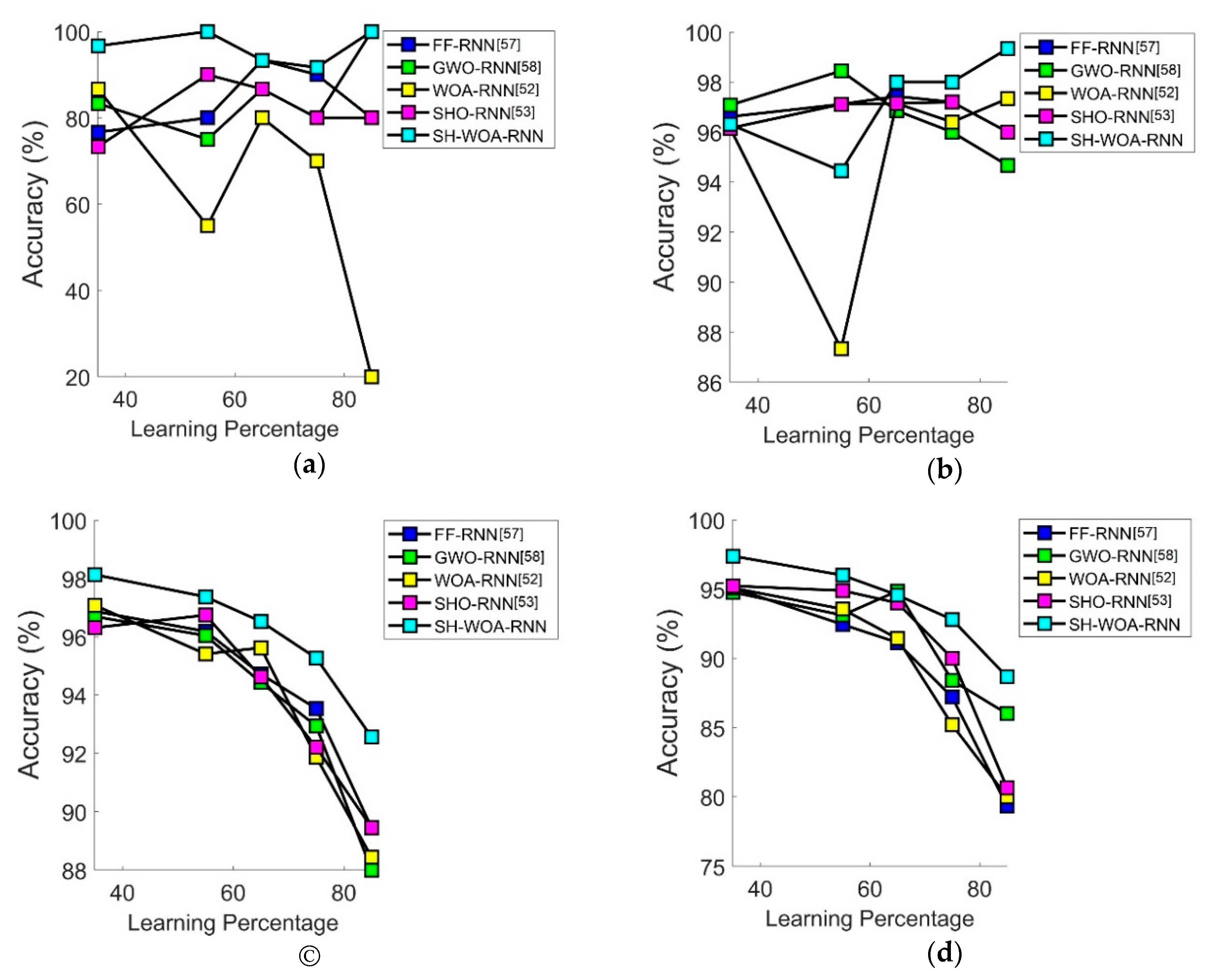
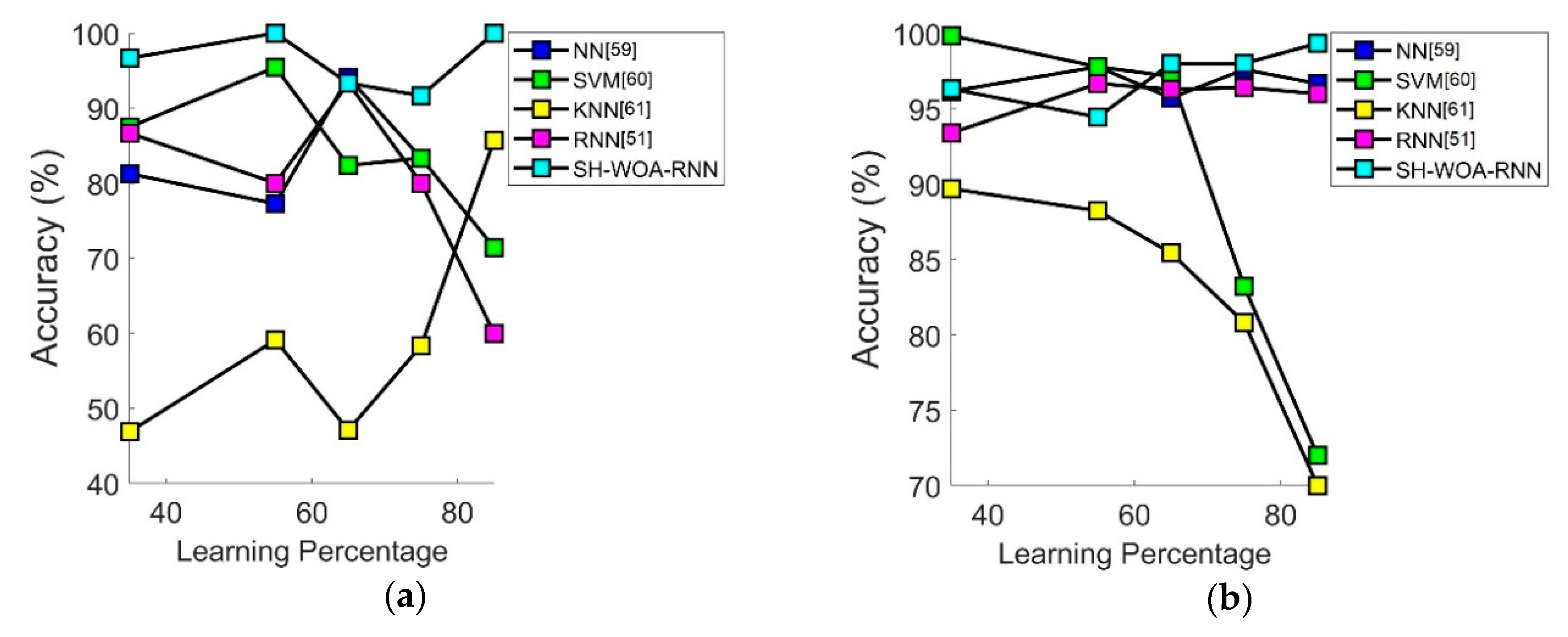
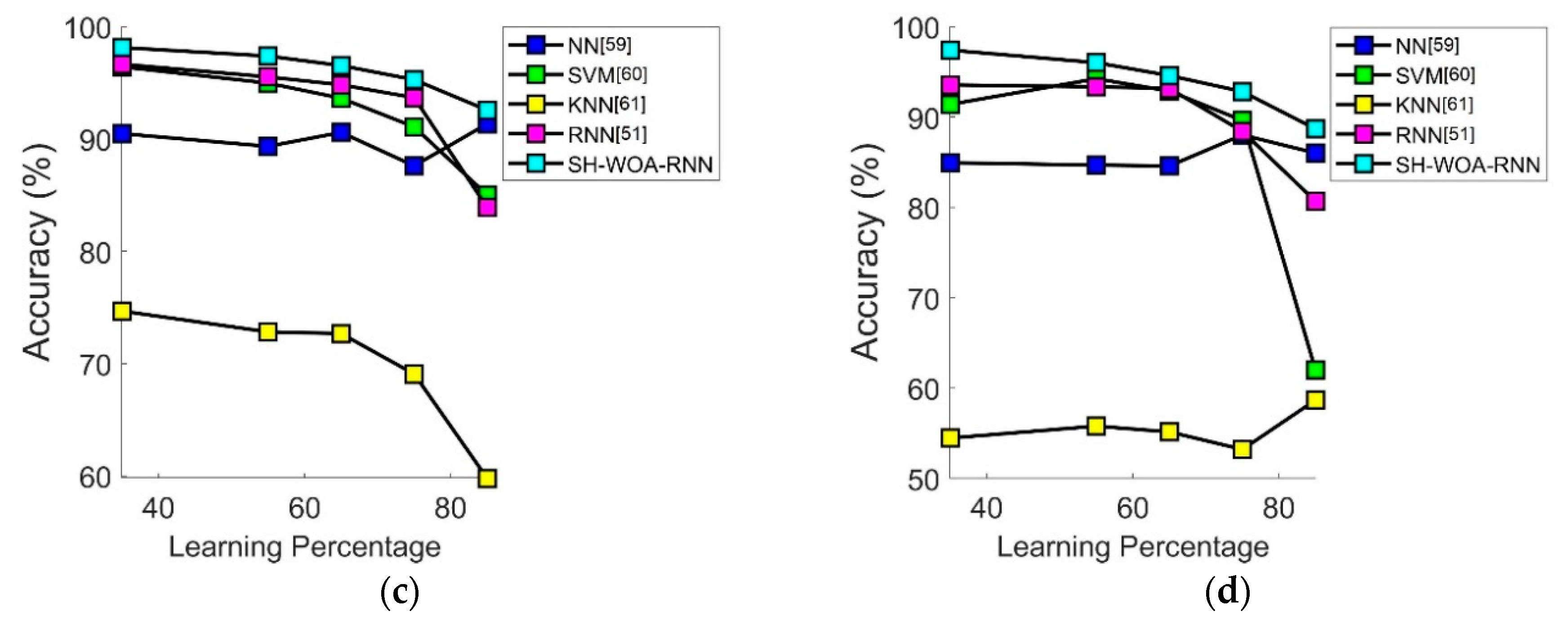
7.3. Performance Analysis in Terms of Accuracy

The performance analysis of the proposed and the conventional heuristic-based RNN with respect to the learning percentages for different datasets is shown in Figure 5. In Figure 5a, the accuracy of the improved SH-WOA-RNN is correctly defined for all the learning percentages. At 35% learning, the accuracy of the introduced SH-WOA-RNN is 15.2%, 19.5%, 25.6%, and 28.9% better than that of the WOA-RNN, GWO-RNN, FF-RNN, and SHO-RNN for the “3D-printer” dataset, respectively. Additionally, the accuracy of the improved SH-WOA-RNN from Figure 5c for the “faulty steel plates” dataset is 3.9%, 5.4%, and 5.6% better than that of the SHO-RNN, WOA-RNN, and GWO-RNN, respectively. The analysis of accuracy for the proposed SH-WOA-RNN and the existing machine learning algorithms is shown in Figure 6. The accuracy of the suggested SH-WOA-RNN for the “3D-printer” dataset is 10.11%, 11.3%, 22.5%, and 51% better than that of the SVM, NN, and KNN at 35% learning, respectively, as shown in Figure 6a. Moreover, in Figure 6c, the accuracy of the recommended SHO-WOA-RNN for the “faulty steel plates” dataset at 35% learning is 2%, 8.8%, and 30.6% better than that of the RNN, NN, and KNN, respectively. Therefore, the proposed SHO-WOA-RNN outperformed the conventional algorithms for mechanical data classification.

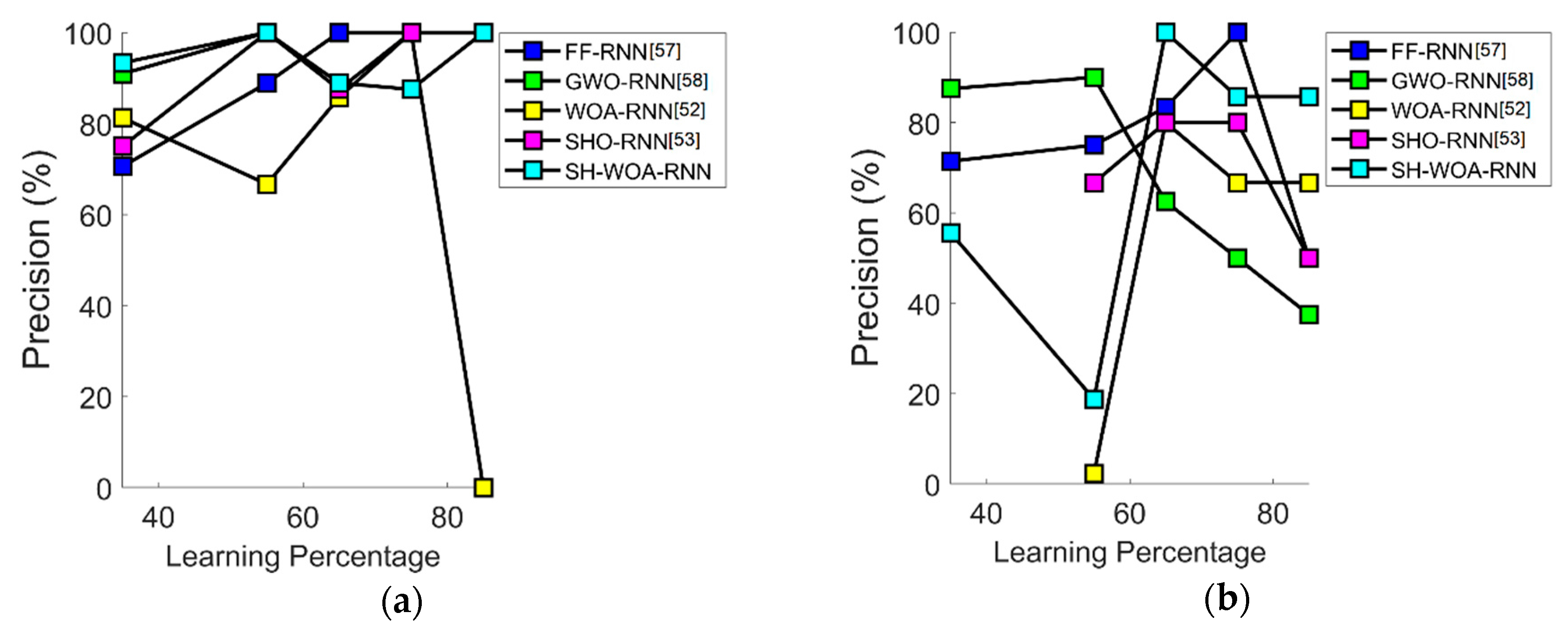
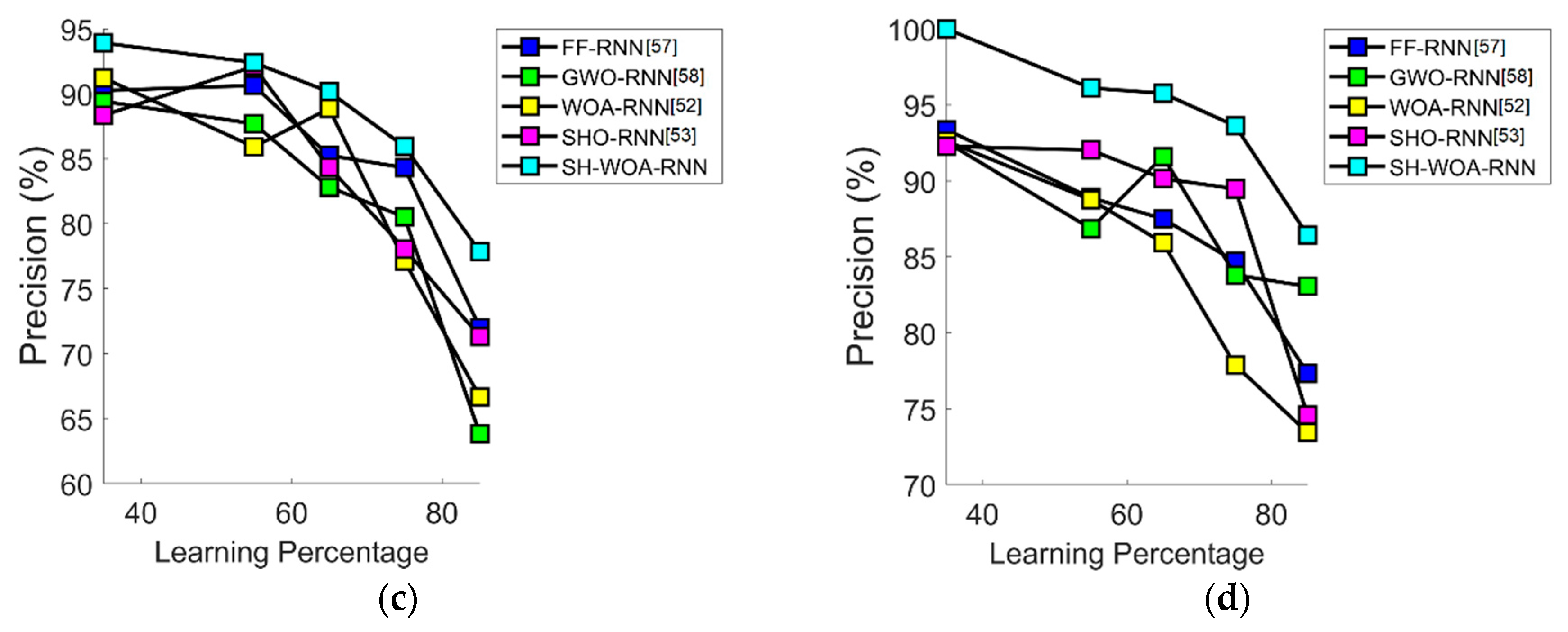
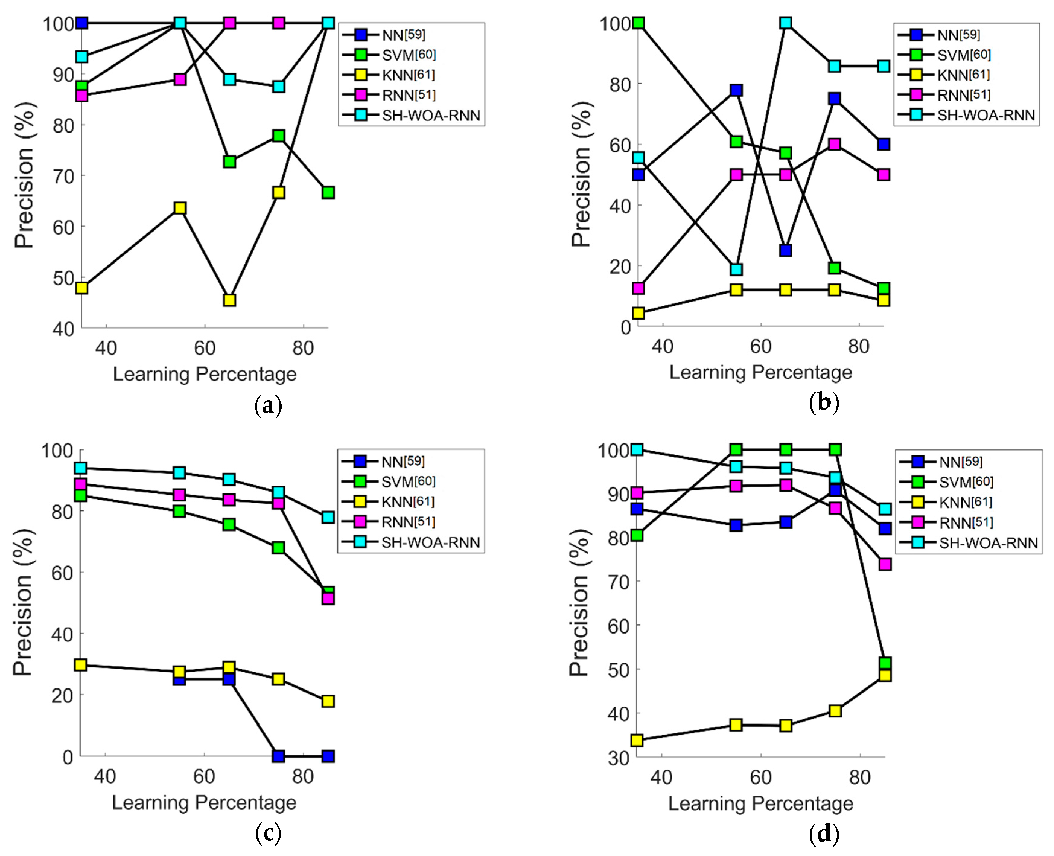
7.4. Performance Analysis in Terms of Precision

Figure 7 shows the performance analysis of the developed and the existing heuristic-based RNN with respect to the learning percentage in terms of precision. As shown in Figure 7b, the precision of the improved SH-WOA-RNN for the “air pressure system failure in the Scania trucks” dataset is 21.4%, 70%, and 50% better than that of the WOA, SHO, and GWO-RNN at 85% learning. When 35% learning is considered for the dataset mechanical data analysis, the precision of the implemented SH-WOA-RNN is 6.3%, 7.5%, and 8.6% better than that of the FF-RNN, WOA-RNN, and SHO-RNN, respectively, as shown in Figure 7d. Moreover, for all the learning percentages, the proposed SH-WOA-RNN performed well for data classification. The classification analysis using the proposed and conventional machine learning algorithms in terms of the precision based on different learning percentages is shown in Figure 8. The precision of the developed SH-WOA-RNN for the “air pressure system failure in the Scania trucks” dataset is 41.6%, 70%, 82.3%, and 88.2% better than that of the NNN, RNN, SVM, and KNN at 85% learning, as shown in Figure 8b. In terms of precision, as shown in Figure 8d, the suggested SH-WOA-RNN for dataset mechanical data analysis is 11.1%, 12.3%, 25%, and 68% better than that of the RNN, NN, SVM, and KNN at 35% learning. Finally, it is concluded that the developed SH-WOA-RNN is suitable for classifying all types of mechanical data.

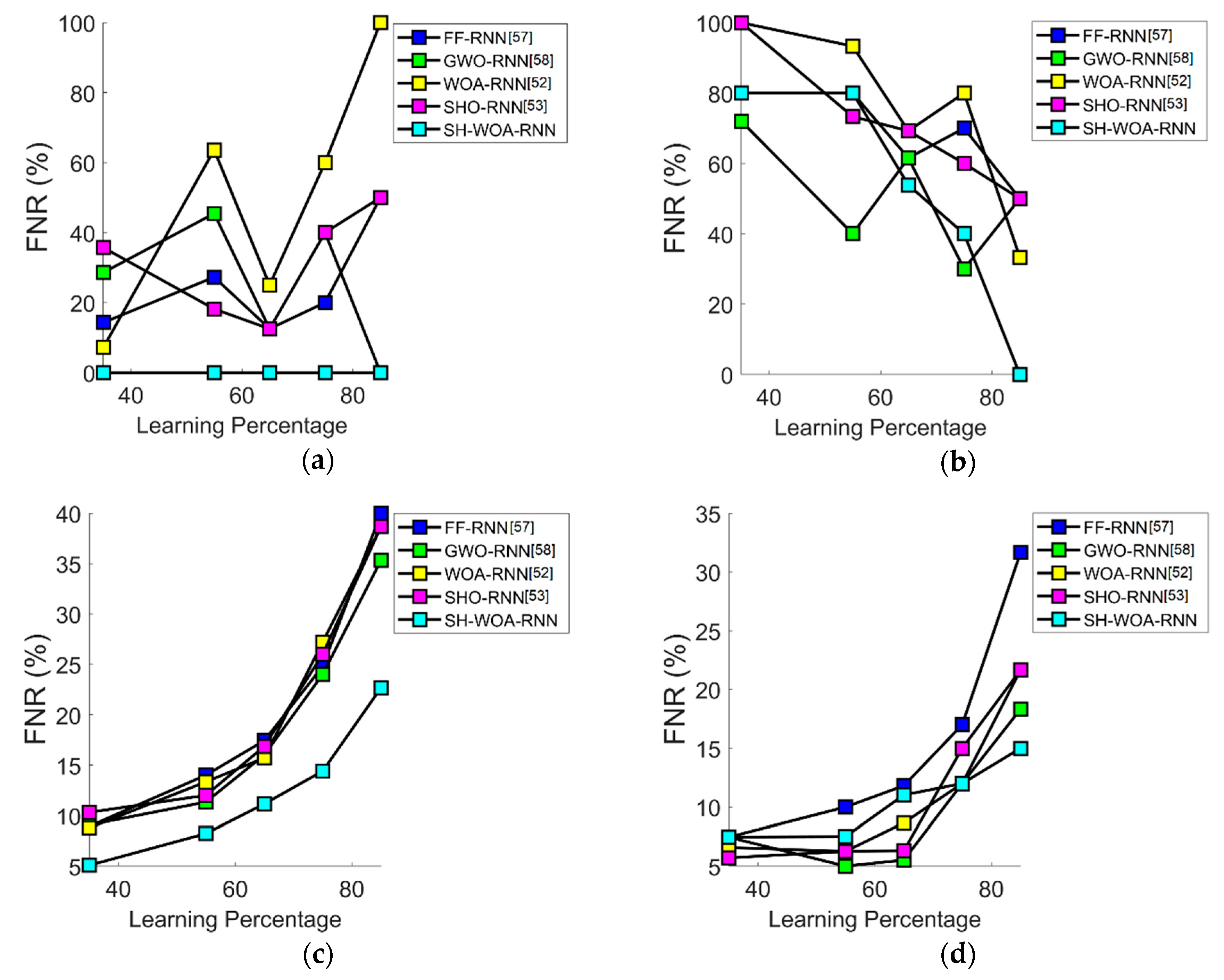
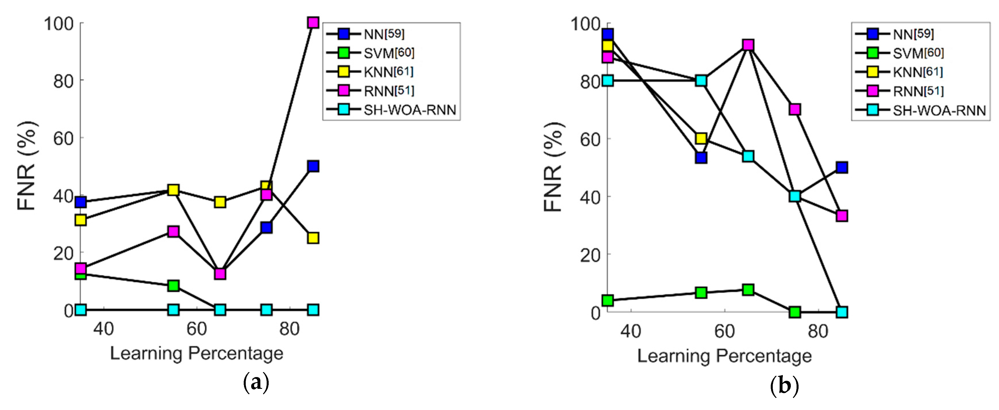
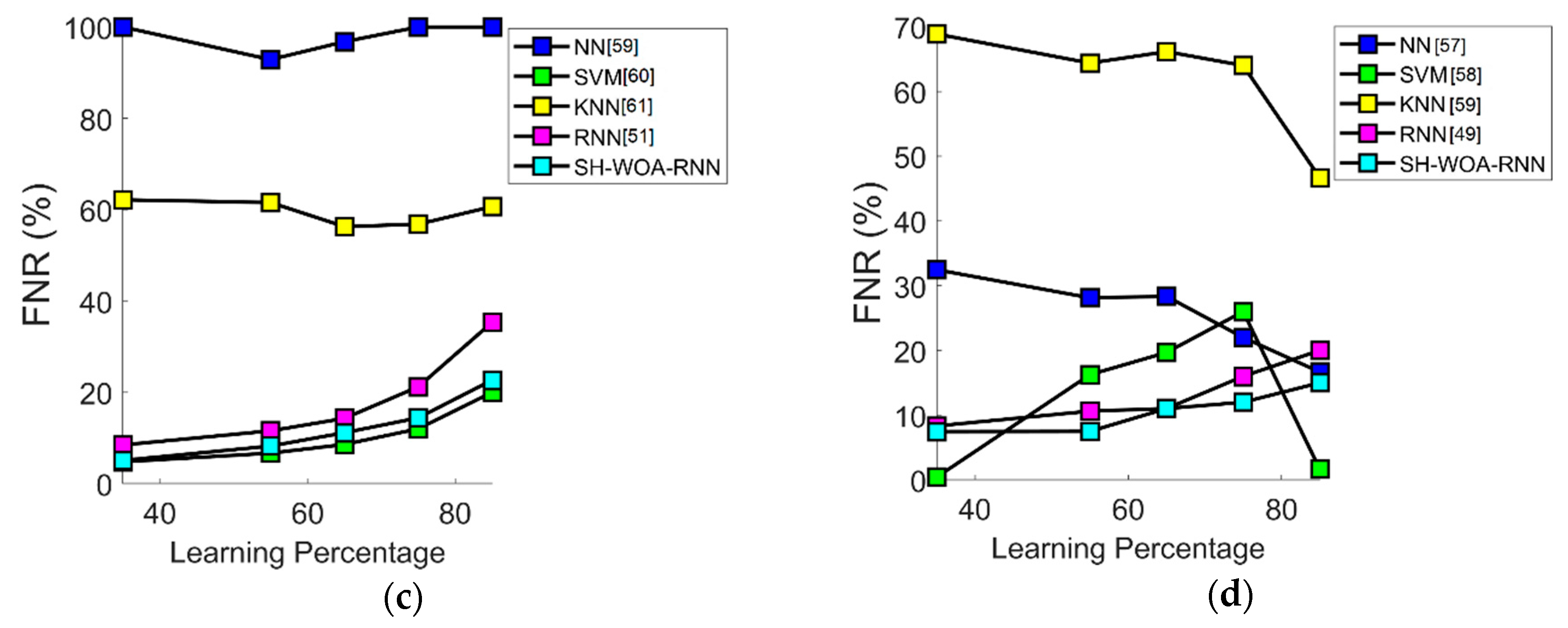
7.5. Performance Analysis in Terms of FNR

The performance analysis of the improved SH-WOA-RNN and other metaheuristic-based RNN in terms of the FNR with respect to the learning percentage is shown in Figure 9. At 35% learning, the FNR of the improved SH-WOA-RNN for the “3D- printer” dataset is 100% better than that of the WOA-RNN, FF-RNN, GWO-RNN, and SHO-RNN, as shown in Figure 9a. Similarly, for all the remaining learning percentages for the “3D-printer” dataset, the performance of the introduced SH-WOA-RNN is extremely high. The FNR of the suggested SH-WOA-RNN at 35% learning for the “all pressure system failure in Scania trucks” dataset is 100% better than that of the WOA-RNN and SHO-RNN, as shown in Figure 9b. In Figure 10, the classification performance in terms of the FNR for the proposed and the existing models is depicted. As shown in Figure 10a, the FNR of the developed SH-WOA-RNN at 35% learning for the “3D-printer” dataset is 100% better than that of the NN, KNN, RNN, and SVM. At all the learning percentages, the proposed SH-WOA-RNN performed well in terms of the FNR. At 85% learning. as shown in Figure 10b, for the “air pressure system failure in the Scania trucks” dataset the FNR of the improved SH-WOA-RNN is 100% better than that of the NN and RNN. Hence, the suggested SH-WOA-RNN is superior to conventional algorithms and performs well in categorizing mechanical data.

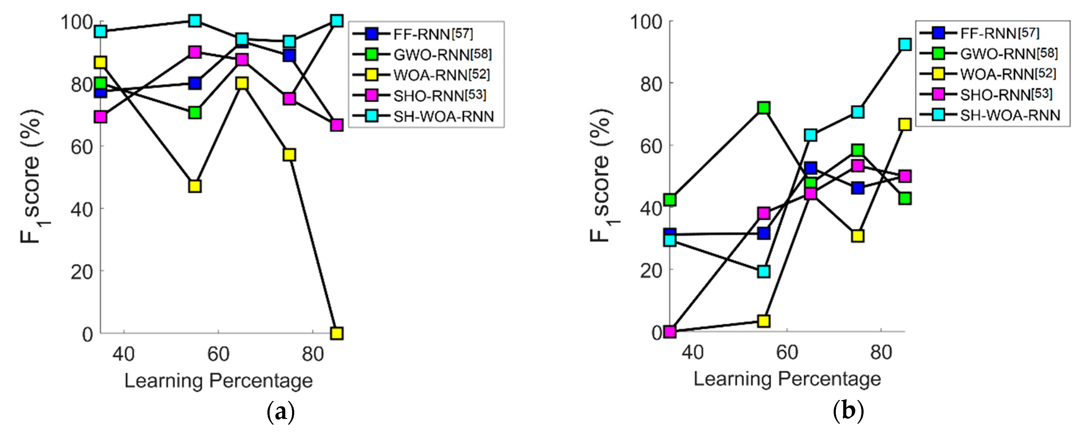
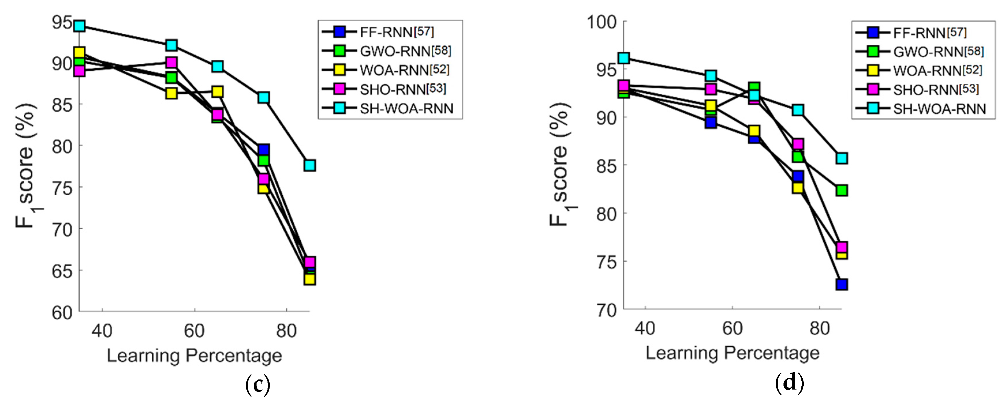
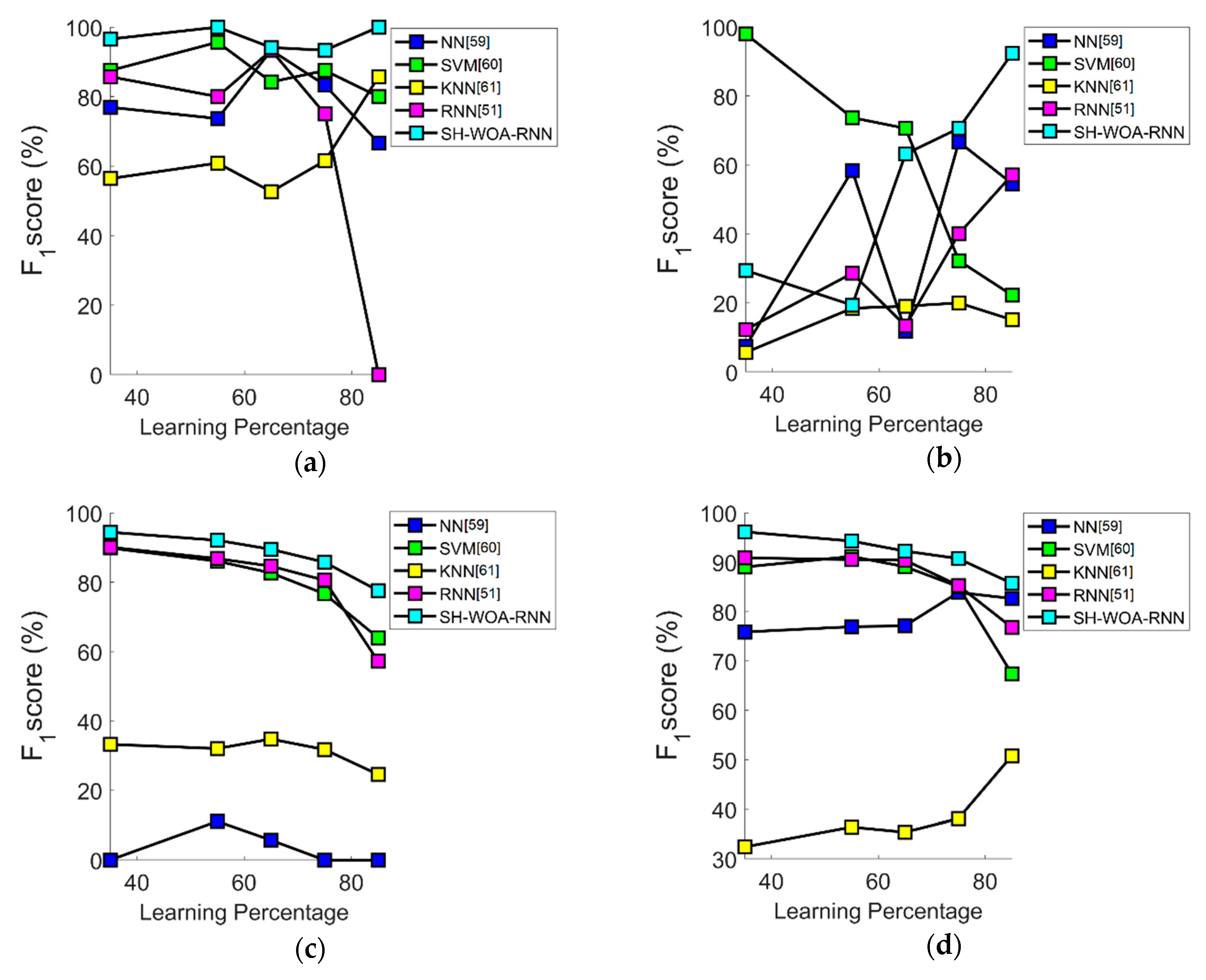
7.6. Performance Analysis in Terms of F1-Score

In Figure 11, the performance evaluation in terms of the F1-score by the improved SH-WOA-RNN and the existing methods with respect to the learning percentage is shown. The F1-score of the modified SH-WOA-RNN for the “faulty steel plates” dataset is 4.3%, 5.5%, and 6.7% better than those of the WOA-RNN, GWO, and SHO-RNN at 35% learning, respectively, as shown in Figure 11c. At 35% learning for the “mechanical analysis data” dataset, the F1-score of the improved SH-WOA-RNN is 2.6% and 3.7% better than that of the SHO-RNN and GWO, respectively, as shown in Figure 11d. The F1-score of the developed SH-WOA-RNN and the other machine learning algorithms is shown in Figure 12. As shown in Figure 12a, the F1-score of the recommended SH-WOA-RNN for the “faulty steel plates” dataset is 23%, 33.3%, 65%, and 100% better than that of the SVM, RNN, KNN, and NN at 85% learning. At 50% learning, the F1-score of the modified SH-WOA-RNN for the “mechanical analysis” dataset is 5.5%, 10.4%, and 63% better than that of the RNN, NN, and KNN, as shown in Figure 12d. Finally, the suggested SH-WOA-RNN is superior to conventional methods and performs well in categorizing mechanical data.

7.7. Overall Performance Analysis

The overall performance analysis of the proposed algorithm and conventional algorithms is shown in Tables 3, 5, 7 and 9 for the “3D-printer”, “air pressure system failure in Scania trucks”, “faulty steel plates”, and “mechanical analysis data” datasets, respectively. Moreover, the classification analysis of the developed SH-WOA-RNN and the conventional classifiers for the four abovementioned datasets are tabulated in Tables 4, 6, 8 and 10, correspondingly. As shown in

Table 3. Overall performance analysis of the proposed and conventional heuristic-based RNN for mechanical data classification using the “3d Printer” dataset.

Performance Metrics	FF-RNN [57]	GWO-RNN [58]	WOA-RNN [52]	SHO-RNN [53]	SH-WOA-RNN
Accuracy	0.9	0.8	0.7	0.8	0.91667
Sensitivity	0.8	0.6	0.4	0.6	1
Specificity	1	1	1	1	0.8
Precision	1	1	1	1	0.875
FPR	0	0	0	0	0.2
FNR	0.2	0.4	0.6	0.4	0
NPV	1	1	1	1	0.8
FDR	0	0	0	0	0.125
F1-Score	0.88889	0.75	0.57143	0.75	0.93333
MCC	0.8165	0.65465	0.5	0.65465	0.83666

, the accuracy of the improved SH-WOA-RNN is 1.8%, 14.5%, and 30.9% better than that of the FF-RNN, GWO and SHO-RNN, and WOA-RNN, respectively. The overall classification analysis of the improved SH-WOA-RNN in terms of accuracy, as shown in

Table 4. Overall performance analysis of the proposed and conventional machine learning algorithms for mechanical data classification using the “3d Printer” dataset.

Performance Metrics	NN [59]	SVM [60]	KNN [61]	RNN [29]	SH-WOA-RNN
Accuracy	0.83333	0.83333	0.58333	0.8	0.91667
Sensitivity	0.71429	1	0.57143	0.6	1
Specificity	1	0.6	0.6	1	0.8
Precision	1	0.77778	0.66667	1	0.875
FPR	0	0.4	0.4	0	0.2
FNR	0.28571	0	0.42857	0.4	0
NPV	1	0.6	0.6	1	0.8
FDR	0	0.22222	0.33333	0	0.125
F1-Score	0.83333	0.875	0.61538	0.75	0.93333
MCC	0.71429	0.68313	0.16903	0.65465	0.83666

, is 10%, 57.1%, and 14.5% better than that of the NN and SVM, KNN, and RNN, respectively. Similarly, as shown in

Table 5. Overall performance analysis of the proposed and conventional heuristic-based RNN for mechanical data classification using the “Air Pressure System Failure in Scania Trucks” dataset.

Performance Metrics	FF-RNN [57]	GWO-RNN [58]	WOA-RNN [52]	SHO-RNN [53]	SH-WOA-RNN
Accuracy	0.972	0.96	0.964	0.972	0.98
Sensitivity	0.3	0.7	0.2	0.4	0.6
Specificity	1	0.97083	0.99583	0.99583	0.99583
Precision	1	0.5	0.66667	0.8	0.85714
FPR	0	0.029167	0.004167	0.004167	0.004167
FNR	0.7	0.3	0.8	0.6	0.4
NPV	1	0.97083	0.99583	0.99583	0.99583
FDR	0	0.5	0.33333	0.2	0.14286
F1-Score	0.46154	0.58333	0.30769	0.53333	0.70588
MCC	0.53991	0.57174	0.35244	0.55405	0.70775

, the accuracy of the proposed SH-WOA-RNN is 0.8%, 2%, and 1.6% better than that of the FF-RNN and SHO-RNN, GWO-RNN, and WOA-RNN, respectively. As shown in

Table 6. Overall performance analysis of the proposed and conventional machine learning algorithms for mechanical data classification using the “Air Pressure System Failure in Scania Trucks” dataset.

Performance Metrics	NN [59]	SVM [60]	KNN [61]	RNN [29]	SH-WOA-RNN
Accuracy	0.976	0.832	0.808	0.964	0.98
Sensitivity	0.6	1	0.6	0.3	0.6
Specificity	0.99167	0.825	0.81667	0.99167	0.99583
Precision	0.75	0.19231	0.12	0.6	0.85714
FPR	0.008333	0.175	0.18333	0.008333	0.004167
FNR	0.4	0	0.4	0.7	0.4
NPV	0.99167	0.825	0.81667	0.99167	0.99583
FDR	0.25	0.80769	0.88	0.4	0.14286
F1-Score	0.66667	0.32258	0.2	0.4	0.70588
MCC	0.65876	0.39831	0.20412	0.40825	0.70775

, the accuracy of the recommended SH-WOA-RNN is 0.4%, 17.7%, 21.2%, and 1.6% better than that of the NN, SVM, KNN, and RNN, respectively. Moreover, the accuracy of the developed SH-WOA-RNN as shown in

Table 7. Overall performance analysis of the proposed and conventional heuristic-based RNN for mechanical data classification using the “Faulty Steel Plates” dataset.

Performance Metrics	FF-RNN [57]	GWO-RNN [58]	WOA-RNN [52]	SHO-RNN [53]	SH-WOA-RNN
Accuracy	0.93533	0.92933	0.91867	0.922	0.95267
Sensitivity	0.752	0.76	0.728	0.74	0.856
Specificity	0.972	0.9632	0.9568	0.9584	0.972
Precision	0.84305	0.80508	0.77119	0.78059	0.85944
FPR	0.028	0.0368	0.0432	0.0416	0.028
FNR	0.248	0.24	0.272	0.26	0.144
NPV	0.972	0.9632	0.9568	0.9584	0.972
FDR	0.15695	0.19492	0.22881	0.21941	0.14056
F1-Score	0.79493	0.78189	0.74897	0.75975	0.85772
MCC	0.75843	0.74021	0.70091	0.7136	0.82933

is 1.8%, 2.5%, 3.7%, and 3.3% better than that of the FF-RNN, GWO-RNN, WOA-RNN, and SHO-RNN, respectively. The accuracy of the proposed SH-WOA-RNN is 8.7%, 4.6%, 37.9%, and 1.7% upgraded compared that of the NN, SVM, KNN, and RNN, respectively, as shown in

Table 8. Overall performance analysis of the proposed and conventional machine learning algorithms for mechanical data classification using the “Faulty Steel Plates” dataset.

Performance Metrics	NN [59]	SVM [60]	KNN [61]	RNN [29]	SH-WOA-RNN
Accuracy	0.876	0.91067	0.69067	0.93667	0.95267
Sensitivity	0	0.88	0.432	0.788	0.856
Specificity	0.97333	0.9168	0.7424	0.9664	0.972
Precision	0	0.67901	0.25116	0.82427	0.85944
FPR	0.026667	0.0832	0.2576	0.0336	0.028
FNR	1	0.12	0.568	0.212	0.144
NPV	0.97333	0.9168	0.7424	0.9664	0.972
FDR	1	0.32099	0.74884	0.17573	0.14056
F1-Score	0	0.76655	0.31765	0.80573	0.85772
MCC	−0.05227	0.7216	0.14373	0.76819	0.82933

. In terms of the accuracy, as shown in

Table 9. Overall performance analysis of the proposed and conventional machine learning algorithms for mechanical data classification using the “Mechanical Data Analysis” dataset.

Performance Metrics	FF-RNN [57]	GWO-RNN [58]	WOA-RNN [52]	SHO-RNN [53]	SH-WOA-RNN
Accuracy	0.872	0.884	0.852	0.9	0.928
Sensitivity	0.83	0.88	0.88	0.85	0.88
Specificity	0.9	0.88667	0.83333	0.93333	0.96
Precision	0.84694	0.8381	0.77876	0.89474	0.93617
FPR	0.1	0.11333	0.16667	0.066667	0.04
FNR	0.17	0.12	0.12	0.15	0.12
NPV	0.9	0.88667	0.83333	0.93333	0.96
FDR	0.15306	0.1619	0.22124	0.10526	0.06383
F1-Score	0.83838	0.85854	0.82629	0.87179	0.90722
MCC	0.73254	0.76098	0.70216	0.79061	0.84957

, the performance of the proposed SH-WOA-RNN is 6.4%, 4.9%, 8.9%, and 3.1% better than that of the FF-RNN, GWO-RNN, WOA-RNN, and SHO-RNN, respectively. Moreover, as shown in

Table 10. Overall performance analysis of the proposed and conventional machine learning algorithms for mechanical data classification using the “Mechanical Data Analysis” dataset.

Performance Metrics	NN [59]	SVM [60]	KNN [61]	RNN [29]	SH-WOA-RNN
Accuracy	0.88	0.896	0.532	0.884	0.928
Sensitivity	0.78	0.74	0.36	0.84	0.88
Specificity	0.94667	1	0.64667	0.91333	0.96
Precision	0.90698	1	0.40449	0.86598	0.93617
FPR	0.053333	0	0.35333	0.086667	0.04
FNR	0.22	0.26	0.64	0.16	0.12
NPV	0.94667	1	0.64667	0.91333	0.96
FDR	0.093023	0	0.59551	0.13402	0.06383
F1-Score	0.83871	0.85057	0.38095	0.85279	0.90722
MCC	0.74939	0.79415	0.006821	0.75736	0.84957

, the accuracy of the improved SH-WOA-RNN is 5.4, 3.5%, 74.4, and 4.9% better than that of the NN, SVM, KNN, and RNN, respectively. Finally, it is confirmed that the suggested SH-WOA-RNN outperformed the conventional algorithms for mechanical data classification.

7.8. Analysis Based on Computational Time

The measurement time of the proposed method and the current methods is evaluated and presented in

Table 11. The computational time of the proposed and existing methods.

Methods	Computational Time (sec.)
	Three-Dimensional (3D) Printer (Test Case 1)	Air Pressure System Failure in Scania Trucks (Test Case 2)	Faulty Steel Plates (Test Case 3)	Mechanical Analysis Data (Test Case 4)
FF [57]	237.41	188.09	191.17	163.55
GWO [58]	169.58	118.5	131.27	102.56
WOA [52]	180.47	95.481	149.66	102.83
SHO [53]	393.53	302.82	303.94	320.8
SH-WOA	88.596	163.4	127.2	168.76

.

The proposed algorithm is better than the current techniques when considering the calculation time, such as FF, GWO, WOA, and SHO. For Testcase_1, the computational time of the proposed SH-WOA is 62.68% better than FF, 47.75% better than GWO, 50.90% better than WOA, and 77.48% better than SHO. For Testcase_2, the computational time of the proposed SH-WOA is 13.12% better than FF, 37.89% better than GWO, 71.13% better than WOA, and 46.04% better than SHO. For Testcase_3, the computational time of the proposed SH-WOA is 33.46% better than FF, 3.10% better than GWO, 15% better than WOA, and 58.14% better than SHO. Similarly, for Testcase_4, the computational time of the proposed SH-WOA is 3.18% better than FF, 64.54% better than GWO, 64.11% better than WOA, and 47.39% better than SHO, respectively.

Complexity of time of the proposed technique using big O notation:

The most famous metric for the measurement of time complexity is the Big O notation. Big O defines the worst-case scenario explicitly and can be used to define the execution time needed or the space an algorithm requires. The time complexity of the proposed SH-WOA is $O \left(i{t}_{max}\ast n{e}^2\right)$, where ne is the population size and $i{t}_{max}$ is the maximum number of iterations.

8. Discussion and Conclusions

In this paper, the performance of the proposed method has been evaluated by metrics such as accuracy, precision, FNR, F1-score, and time complexity. Moreover, the efficacy of the proposed technique was compared with that of the current methods, such as NN, SVM, KNN, and RNN. All the mentioned algorithms were coded by us and the same problem was fed to each of them on the same computer to gain unbiased results in terms of the performance measures. The study showed that the proposed approach provides a better performance relative to the other comparative methods. The possible reasons behind the high performance of the proposed method can be attributed to the hybridization.

The proposed SH-WOA is the integration of WOA and SHO. The advantages of SHO include its faster convergence rate, being easy to implement, its strong global search, its simplicity, and its accuracy. The benefits of WOA include its low complexity, high speed, robustness, increased machine efficiency, improved product quality, increased system reliability, advantages in solving clustering problems, limited number of parameters, and lack of a local optima trap. The advantages of RNN include that it can process any length of input and it is popular and successful for variable length representation such as sequences and images. Therefore, the amalgamation of these techniques resulted in an efficient and efficacious algorithm for data classification.

In this research work, a new model has been developed for implementing in a data classification problem. The datasets are based on various mechanical maintenance data. The introduced method comprised four phases: data acquisition, feature extraction, feature selection, and classification. For data acquisition, four datasets—i.e., “3D printer”, “air pressure system failure in Scania trucks”, “faulty steel plates”, and “mechanical data analysis”—were gathered from popular data repositories. To categorize the datasets, the attributes of each dataset were considered for further processing. In the feature extraction phase, PCA, as well as the first- and higher-order statistical features, were extracted. Moreover, feature selection was performed to reduce the dimensions of the features for an error-free classification. To perform a feature selection, a new model called the SH-WOA was employed. The selected features were subjected to a deep learning model—i.e., the RNN. The number of hidden neurons in the RNN was optimized to enhance the performance of the RNN using the introduced SH-WOA. Hence, the performance of the suggested model was evaluated and validated using all the datasets. The results indicated that the accuracy of the improved SH-WOA-RNN was 1.8%, 14.5%, and 30.9% better than that of the FF-RNN, SH-WOA-RNN, and WOA-RNN for the “air pressure system failure in Scania trucks” dataset, respectively. Hence, it is concluded that the suggested SH-WOA is suitable and effective for the data classification of mechanical systems maintenance. The proposed SH-WOA has not been tested much for solving other complex problems in the literature yet. The advantages of the proposed method include its low complexity, high speed, robustness, increased machine efficiency, improved product quality, increased system reliability, and improved rate of production. The drawbacks consist of a high initial set up cost, poor performance in exploring the search space, and more complicated system. Therefore, in the future we will develop a multiple input multiple output (MIMO)-based module for the better performance of the system and will try to mitigate the disadvantages and limitations. Moreover, the developed system will be tested with Dejong’s functions.

References

1. Lei, Y.; Lin, J.; He, Z.; Zuo, M.J. A review on empirical mode decomposition in fault diagnosis of rotating machinery. Mech. Syst. Signal Process. 2013, 35, 108–126. [Google Scholar] [CrossRef]
2. El Kadiri, S.; Grabot, B.; Thoben, K.-D.; Hribernik, K.; Emmanouilidis, C.; von Cieminski, G.; Kiritsis, D. Current trends on ICT technologies for enterprise information systems. Comput. Ind. 2016, 79, 14–33. [Google Scholar] [CrossRef] [Green Version]
3. Precup, R.-E.; Angelov, P.; Costa, B.S.J.; Sayed-Mouchaweh, M. An overview on fault diagnosis and nature-inspired optimal control of industrial process applications. Comput. Ind. 2015, 74, 75–94. [Google Scholar] [CrossRef]
4. Miyajima, R. Deep Learning Triggers a New Era in Industrial Robotics. IEEE MultiMedia 2017, 24, 91–96. [Google Scholar] [CrossRef]
5. Li, Z.; Wang, Y.; Wang, K.-S. Intelligent predictive maintenance for fault diagnosis and prognosis in machine centers: Industry 4.0 scenario. Adv. Manuf. 2017, 5, 377–387. [Google Scholar] [CrossRef]
6. Lu, C.; Wang, Z.-Y.; Qin, W.-L.; Ma, J. Fault diagnosis of rotary machinery components using a stacked denoising autoencoder-based health state identification. Signal Process. 2017, 130, 377–388. [Google Scholar] [CrossRef]
7. Lin, J.; Chen, Q. A novel method for feature extraction using crossover characteristics of nonlinear data and its application to fault diagnosis of rotary machinery. Mech. Syst. Signal Process. 2014, 48, 174–187. [Google Scholar] [CrossRef]
8. Stimpson, A.J.; Cummings, M.L. Assessing Intervention Timing in Computer-Based Education Using Machine Learning Algorithms. IEEE Access 2014, 2, 78–87. [Google Scholar] [CrossRef]
9. Michalski, R.S.; Carbonell, J.G.; Mitchell, T.M. Machine Learning an Artificial Intelligence Approach, 1st ed.; Springer: Berlin/Heidelberg, Germany, 1983; p. 572. [Google Scholar]
10. Wang, Z.-Y.; Lu, C.; Zhou, B. Fault diagnosis for rotary machinery with selective ensemble neural networks. Mech. Syst. Signal. Process. 2018, 113, 112–130. [Google Scholar] [CrossRef]
11. Lu, P.; Chen, S.; Zheng, Y. Artificial intelligence in civil engineering. Math. Probelms Eng. 2012, 2012, 1–22. [Google Scholar] [CrossRef] [Green Version]
12. Krummenacher, G.; Ong, C.S.; Koller, S.; Kobayashi, S.; Buhmann, J.M. Wheel Defect Detection With Machine Learning. IEEE Trans. Intell. Transp. Syst. 2018, 19, 1176–1187. [Google Scholar] [CrossRef]
13. Lei, Y.; Jia, F.; Lin, J.; Xing, S.; Ding, S.X. An Intelligent Fault Diagnosis Method Using Unsupervised Feature Learning Towards Mechanical Big Data. IEEE Trans. Ind. Electron. 2016, 63, 3137–3147. [Google Scholar] [CrossRef]
14. Yang, Y.; Dong, X.J.; Peng, Z.K.; Zhang, W.M.; Meng, G. Vibration signal analysis using parameterized time–frequency method for features extraction of varying-speed rotary machinery. J. Sound Vib. 2015, 335, 350–366. [Google Scholar] [CrossRef]
15. Zhou, L.; Ma, L. Extreme Learning Machine-Based Heterogeneous Domain Adaptation for Classification of Hyperspectral Images. IEEE Geosci. Remote Sens. Lett. 2019, 16, 1781–1785. [Google Scholar] [CrossRef]
16. Zhang, C.; Tan, K.C.; Li, H.; Hong, G.S. A Cost-Sensitive Deep Belief Network for Imbalanced Classification. IEEE Trans. Neural Netw. Learn. Syst. 2019, 30, 109–122. [Google Scholar] [CrossRef] [Green Version]
17. Shi, C.; Panoutsos, G.; Luo, B.; Liu, H.; Li, B.; Lin, X. Using Multiple-Feature-Spaces-Based Deep Learning for Tool Condition Monitoring in Ultraprecision Manufacturing. IEEE Trans. Ind. Electron. 2019, 66, 3794–3803. [Google Scholar] [CrossRef] [Green Version]
18. Ruiz-Sarmiento, J.-R.; Monroy, J.; Moreno, F.-A.; Galindo, C.; Bonelo, J.-M.; Gonzalez-Jimenez, J. A predictive model for the maintenance of industrial machinery in the context of industry 4.0. Eng. Appl. Artif. Intell. 2020, 87, 103289. [Google Scholar] [CrossRef]
19. Abidi, M.H.; Alkhalefah, H.; Mohammed, M.K.; Umer, U.; Qudeiri, J.E.A. Optimal Scheduling of Flexible Manufacturing System Using Improved Lion-Based Hybrid Machine Learning Approach. IEEE Access 2020, 8, 96088–96114. [Google Scholar] [CrossRef]
20. Naik, D.L.; Kiran, R. Naïve Bayes classifier, multivariate linear regression and experimental testing for classification and characterization of wheat straw based on mechanical properties. Ind. Crops Prod. 2018, 112, 434–448. [Google Scholar] [CrossRef]
21. Xiong, S.; Fu, Y.; Ray, A. Bayesian Nonparametric Regression Modeling of Panel Data for Sequential Classification. IEEE Trans. Neural Netw. Learn. Syst. 2018, 29, 4128–4139. [Google Scholar] [CrossRef]
22. McArthur, J.J.; Shahbazi, N.; Fok, R.; Raghubar, C.; Bortoluzzi, B.; An, A. Machine learning and BIM visualization for maintenance issue classification and enhanced data collection. Adv. Eng. Inform. 2018, 38, 101–112. [Google Scholar] [CrossRef]
23. Konstantopoulos, G.; Koumoulos, E.P.; Charitidis, C.A. Classification of mechanism of reinforcement in the fiber-matrix interface: Application of Machine Learning on nanoindentation data. Mater. Des. 2020, 192, 108705. [Google Scholar] [CrossRef]
24. Maxwell, K.; Rajabi, M.; Esterle, J. Automated classification of metamorphosed coal from geophysical log data using supervised machine learning techniques. Int. J. Coal Geol. 2019, 214, 103284. [Google Scholar] [CrossRef]
25. Islam, M.M.; Rahman, M.J.; Chandra Roy, D.; Maniruzzaman, M. Automated detection and classification of diabetes disease based on Bangladesh demographic and health survey data, 2011 using machine learning approach. Diabetes Metab. Syndr. Clin. Res. Rev. 2020, 14, 217–219. [Google Scholar] [CrossRef] [PubMed]
26. Karandikar, J. Machine learning classification for tool life modeling using production shop-floor tool wear data. Procedia Manuf. 2019, 34, 446–454. [Google Scholar] [CrossRef]
27. Li, Z.; Wang, Y.; Wang, K. A deep learning driven method for fault classification and degradation assessment in mechanical equipment. Comput. Ind. 2019, 104, 1–10. [Google Scholar] [CrossRef]
28. Siam, A.; Ezzeldin, M.; El-Dakhakhni, W. Machine learning algorithms for structural performance classifications and predictions: Application to reinforced masonry shear walls. Structures 2019, 22, 252–265. [Google Scholar] [CrossRef]
29. Chen, X.; Zhang, L.; Liu, T.; Kamruzzaman, M.M. Research on deep learning in the field of mechanical equipment fault diagnosis image quality. J. Vis. Commun. Image Represent. 2019, 62, 402–409. [Google Scholar] [CrossRef]
30. Mahmodi, K.; Mostafaei, M.; Mirzaee-Ghaleh, E. Detection and classification of diesel-biodiesel blends by LDA, QDA and SVM approaches using an electronic nose. Fuel 2019, 258, 116114. [Google Scholar] [CrossRef]
31. Zhu, X.; Cai, Z.; Wu, J.; Cheng, Y.; Huang, Q. Convolutional neural network based combustion mode classification for condition monitoring in the supersonic combustor. Acta Astronaut. 2019, 159, 349–357. [Google Scholar] [CrossRef]
32. Akyol, S.; Alatas, B. Sentiment classification within online social media using whale optimization algorithm and social impact theory based optimization. Phys. A Stat. Mech. Appl. 2020, 540, 123094. [Google Scholar] [CrossRef]
33. Agrawal, R.K.; Kaur, B.; Sharma, S. Quantum based Whale Optimization Algorithm for wrapper feature selection. Appl. Soft Comput. 2020, 89, 106092. [Google Scholar] [CrossRef]
34. Devaraj, A.F.S.; Elhoseny, M.; Dhanasekaran, S.; Lydia, E.L.; Shankar, K. Hybridization of firefly and Improved Multi-Objective Particle Swarm Optimization algorithm for energy efficient load balancing in Cloud Computing environments. J. Parallel Distrib. Comput. 2020, 142, 36–45. [Google Scholar] [CrossRef]
35. Gölcük, İ.; Ozsoydan, F.B. Evolutionary and adaptive inheritance enhanced Grey Wolf Optimization algorithm for binary domains. Knowl. Based Syst. 2020, 194, 105586. [Google Scholar] [CrossRef]
36. Liu, M.; Yao, X.; Li, Y. Hybrid whale optimization algorithm enhanced with Lévy flight and differential evolution for job shop scheduling problems. Appl. Soft Comput. 2020, 87, 105954. [Google Scholar] [CrossRef]
37. Dhiman, G.; Kumar, V. Multi-objective spotted hyena optimizer: A Multi-objective optimization algorithm for engineering problems. Knowl. Based Syst. 2018, 150, 175–197. [Google Scholar] [CrossRef]
38. Xin-gang, Z.; Ji, L.; Jin, M.; Ying, Z. An improved quantum particle swarm optimization algorithm for environmental economic dispatch. Expert Syst. Appl. 2020, 152, 113370. [Google Scholar] [CrossRef]
39. He, H.; Tan, Y.; Ying, J.; Zhang, W. Strengthen EEG-based emotion recognition using firefly integrated optimization algorithm. Appl. Soft Comput. 2020, 94, 106426. [Google Scholar] [CrossRef]
40. Ranjini, K.S.S.; Murugan, S. Memory based Hybrid Dragonfly Algorithm for numerical optimization problems. Expert Syst. Appl. 2017, 83, 63–78. [Google Scholar] [CrossRef]
41. Tuba, E.; Strumberger, I.; Bezdan, T.; Bacanin, N.; Tuba, M. Classification and Feature Selection Method for Medical Datasets by Brain Storm Optimization Algorithm and Support Vector Machine. Procedia Comput. Sci. 2019, 162, 307–315. [Google Scholar] [CrossRef]
42. Orrù, P.F.; Zoccheddu, A.; Sassu, L.; Mattia, C.; Cozza, R.; Arena, S. Machine Learning Approach Using MLP and SVM Algorithms for the Fault Prediction of a Centrifugal Pump in the Oil and Gas Industry. Sustainability 2020, 12, 4776. [Google Scholar] [CrossRef]
43. Ghafil, H.N.; Jármai, K. Dynamic differential annealed optimization: New metaheuristic optimization algorithm for engineering applications. Appl. Soft Comput. 2020, 93, 106392. [Google Scholar] [CrossRef]
44. Mahjoubi, S.; Barhemat, R.; Bao, Y. Optimal placement of triaxial accelerometers using hypotrochoid spiral optimization algorithm for automated monitoring of high-rise buildings. Autom. Constr. 2020, 118, 103273. [Google Scholar] [CrossRef]
45. Sahal, R.; Breslin, J.G.; Ali, M.I. Big data and stream processing platforms for Industry 4.0 requirements mapping for a predictive maintenance use case. J. Manuf. Syst. 2020, 54, 138–151. [Google Scholar] [CrossRef]
46. Zhou, Q.; Jacobson, A. Thingi10K: A Dataset of 10,000 3D-Printing Models. arXiv. 2016. Available online: https://arxiv.org/abs/1605.04797 (accessed on 20 July 2020).
47. Lindgren, T.; Biteus, J. APS Failure at Scania Trucks Data Set. Scania CV AB, S., Sweden. UCL Machine Learning Repository. Irvine, CA. 2017. Available online: https://archive.ics.uci.edu/ml/datasets/APS+Failure+at+Scania+Trucks (accessed on 20 July 2020).
48. Semeion. Steel Plates Faults Data Set. Research Center of Sciences of Communication, R., Italy. UCL Machine Learning Repository. Irvine, CA. 2010. Available online: https://archive.ics.uci.edu/ml/datasets/Steel+Plates+Faults (accessed on 20 July 2020).
49. Bergadano, F.; Giordana, A.; Saitta, L.; Bracadori, F.; Marchi, D. Mechanical Analysis Data Set. Repository, U.M.L.University of California, School of Information and Computer Science. Irvine, CA. 1990. Available online: https://archive.ics.uci.edu/ml/datasets/Mechanical+Analysis (accessed on 20 July 2020).
50. Xingfu, Z.; Xiangmin, R. Two Dimensional Principal Component Analysis based Independent Component Analysis for face recognition. In Proceedings of the 2011 International Conference on Multimedia Technology, Hangzhou, China, 26–28 July 2011; pp. 934–936. [Google Scholar]
51. Li, F.; Liu, M. A hybrid Convolutional and Recurrent Neural Network for Hippocampus Analysis in Alzheimer’s Disease. J. Neurosci. Methods 2019, 323, 108–118. [Google Scholar] [CrossRef]
52. Mirjalili, S.; Lewis, A. The Whale Optimization Algorithm. Adv. Eng. Softw. 2016, 95, 51–67. [Google Scholar] [CrossRef]
53. Dhiman, G.; Kumar, V. Spotted hyena optimizer: A novel bio-inspired based metaheuristic technique for engineering applications. Adv. Eng. Softw. 2017, 114, 48–70. [Google Scholar] [CrossRef]
54. Boothalingam, R. Optimization using lion algorithm: A biological inspiration from lion’s social behavior. Evol. Intell. 2018, 11, 31–52. [Google Scholar] [CrossRef]
55. Rajakumar, B.R. Lion algorithm for standard and large scale bilinear system identification: A global optimization based on Lion’s social behavior. In Proceedings of the 2014 IEEE Congress on Evolutionary Computation (CEC), Beijing, China, 6–11 July 2014; pp. 2116–2123. [Google Scholar]
56. Beno, M.M.; Rajakumar, B.R. Threshold prediction for segmenting tumour from brain MRI scans. Int. J. Imaging Syst. Technol. 2014, 24, 129–137. [Google Scholar] [CrossRef]
57. Gandomi, A.H.; Yang, X.S.; Talatahari, S.; Alavi, A.H. Firefly algorithm with chaos. Commun. Nonlinear Sci. Numer. Simul. 2013, 18, 89–98. [Google Scholar] [CrossRef]
58. Mirjalili, S.; Mirjalili, S.M.; Lewis, A. Grey Wolf Optimizer. Adv. Eng. Softw. 2014, 69, 46–61. [Google Scholar] [CrossRef] [Green Version]
59. Fernández-Navarro, F.; Carbonero-Ruz, M.; Alonso, D.B.; Torres-Jiménez, M. Global Sensitivity Estimates for Neural Network Classifiers. IEEE Trans. Neural Netw. Learn. Syst. 2017, 28, 2592–2604. [Google Scholar] [CrossRef] [PubMed]
60. Yu, S.; Tan, K.K.; Sng, B.L.; Li, S.; Sia, A.T.H. Lumbar Ultrasound Image Feature Extraction and Classification with Support Vector Machine. Ultrasound Med. Biol. 2015, 41, 2677–2689. [Google Scholar] [CrossRef] [PubMed]
61. Chen, Y.; Hu, X.; Fan, W.; Shen, L.; Zhang, Z.; Liu, X.; Du, J.; Li, H.; Chen, Y.; Li, H. Fast density peak clustering for large scale data based on kNN. Knowl. Based Syst. 2020, 187, 104824. [Google Scholar] [CrossRef]
Figure 1. Architecture of the proposed data classification model.
Mathematics 08 02008 g001
Figure 2. Feature selection and classification by the proposed SH-WOA for mechanical data classification.
Mathematics 08 02008 g002
Figure 3. Solution encoding for feature selection and classification for the proposed mechanical data classification.
Mathematics 08 02008 g003
Figure 4. Flow chart of the proposed SH-WOA for mechanical data classification.
Mathematics 08 02008 g004
Figure 5. Accuracy analysis of proposed and conventional heuristic-based RNN for mechanical data classification using four datasets: (a) 3D printer, (b) air pressure system failure in scania trucks, (c) faulty steel plates, and (d) mechanical analysis data.
Mathematics 08 02008 g005
Figure 6. Accuracy analysis of the proposed and conventional machine learning algorithm for mechanical data classification using four datasets: (a) 3D printer, (b) air pressure system failure in scania trucks, (c) faulty steel plates, and (d) mechanical analysis data.
Mathematics 08 02008 g006aMathematics 08 02008 g006b
Figure 7. Precision analysis of proposed and conventional heuristic-based RNN for mechanical data classification using four datasets: (a) 3D printer, (b) air pressure system failure in scania trucks, (c) faulty steel plates, and (d) mechanical analysis data.
Mathematics 08 02008 g007aMathematics 08 02008 g007b
Figure 8. Precision analysis of proposed and conventional machine learning algorithm for mechanical data classification using four datasets: (a) 3D printer, (b) air pressure system failure in scania trucks, (c) faulty steel plates, and (d) mechanical analysis data.
Mathematics 08 02008 g008
Figure 9. FNR analysis of the proposed and conventional heuristic-based RNN for mechanical data classification using four datasets: (a) 3D printer, (b) air pressure system failure in scania trucks, (c) faulty steel plates, and (d) mechanical analysis data.
Mathematics 08 02008 g009
Figure 10. FNR analysis of the proposed and conventional machine learning algorithm for mechanical data classification using four datasets: (a) 3D printer, (b) air pressure system failure in scania trucks, (c) faulty steel plates, and (d) mechanical analysis data.
Mathematics 08 02008 g010aMathematics 08 02008 g010b
Figure 11. F1-score analysis of the proposed and conventional heuristic-based RNN for mechanical data classification using four datasets: (a) 3D printer, (b) Air pressure system failure in scania trucks, (c) faulty steel plates, and (d) mechanical analysis data.
Mathematics 08 02008 g011aMathematics 08 02008 g011b
Figure 12. F1-score analysis of the proposed and conventional machine learning algorithm for mechanical data classification using four datasets: (a) 3D printer, (b) air pressure system failure in scania trucks, (c) faulty steel plates, and (d) mechanical analysis data.
Mathematics 08 02008 g012