A Phenomenological Epidemic Model Based On the Spatio-Temporal Evolution of a Gaussian Probability Density Function

Abstract

A novel phenomenological epidemic model is proposed to characterize the state of infectious diseases and predict their behaviors. This model is given by a new stochastic partial differential equation that is derived from foundations of statistical physics. The analytical solution of this equation describes the spatio-temporal evolution of a Gaussian probability density function. Our proposal can be applied to several epidemic variables such as infected, deaths, or admitted-to-the-Intensive Care Unit (ICU). To measure model performance, we quantify the error of the model fit to real time-series datasets and generate forecasts for all the phases of the COVID-19, Ebola, and Zika epidemics. All parameters and model uncertainties are numerically quantified. The new model is compared with other phenomenological models such as Logistic Grow, Original, and Generalized Richards Growth models. When the models are used to describe epidemic trajectories that register infected individuals, this comparison shows that the median RMSE error and standard deviation of the residuals of the new model fit to the data are lower than the best of these growing models by, on average, 19.6% and 35.7%, respectively. Using three forecasting experiments for the COVID-19 outbreak, the median RMSE error and standard deviation of residuals are improved by the performance of our model, on average by 31.0% and 27.9%, respectively, concerning the best performance of the growth models.

1. Introduction

During the period of an epidemic when the human-to-human transmission is established, and the number of reported cases and deaths are relevant or watched with alarm, nowcasting and forecasting are of crucial importance for public health planning [1,2]. In this situation, mathematical epidemiological models play a key role in policy decisions about the prevention and control of infectious diseases.

Phenomenological epidemic models characterize and forecast the observed effects of epidemics without postulating biological mechanisms and conjectures that explain the observed phenomena [3,4,5]. In this paper, we propose a new phenomenological epidemic model that is constructed from principles of statistical physics [6].

A random process $y\left(t\right)$ is said to be Markov if and only if all of its future probabilities are determined by its most recently known value. An example of a Markov process is the x component of velocity $v_x\left(t\right)$ of a dust particle in an arbitrarily large room, filled with constant-temperature air. The molecules’ motion is due to random buffeting by other molecules that are uncorrelated [6].

An epidemic may be considered a Markov process because a susceptible individual becomes infected due to successful random contact with an infectious individual. When an infection is successful, it is unrelated to earlier infections.

Our model is based on a partial differential equation (PDE) that is derived from assuming that the spread of infectious diseases is a stationary Markov random process in the statistical-physics sense. This new model is compared to three phenomenological models that are used in fitting real epidemic datasets. Based on this comparative analysis of models, we conclude that our proposal is more flexible to describe some of the trajectories of COVID-19, Ebola, and Zika epidemic outbreaks than other phenomenological models.

The structure of this paper is as follows. In Section 2, the related work is introduced. Section 3 presents the new mathematical model. In Section 4, a numerical model to describe real epidemic situations is proposed. Section 5 describes the experimental setup. The quantitative results of four phenomenological models for the epidemic outbreaks are discussed in Section 6. Conclusions and future work are presented in Section 7. This paper includes an appendix that provides the derivation of the stochastic partial differential equation.

2. Related Work

Several classifications that are widely accepted and good reviews of mathematical epidemic models can be encountered in the literature [7]. Some of the main groups of models that have been established are: mechanistic, compartmental, phenomenological, deterministic, and stochastic.

Due to the existence of characteristics assigned to various model groups, some epidemic models have been classified into hybrid groups. Some examples of hybrid models are the following: mechanistic compartmental models [4], compartmental stochastic models [8], phenomenological stochastic models [9], or mixed deterministic/stochastic models [3].

Mechanistic models incorporate key physical laws or assume biological mechanisms involved in the dynamics of disease transmission to explain patterns in the observed data as well as estimate key transmission parameters such as the basic reproduction number [4].

In compartmental epidemic models, all individuals in the population are classified for each time according to one disease status or compartment, for example: susceptible (S), infected (I), recovered (R), deaths (D), etc. The number of different compartments characterizes the model. Individuals can move into and out of each compartment. For example, at random times, an individual in compartment S changes his classification and belongs to the class I when an individual in compartment I transfers him the infection. A set of linked equations describe the evolution of the number of individuals in each compartment [4,10,11].

Deterministic models describe the evolution of epidemics as a set of equations in such a way that, given a full characterization of the epidemic at any time t, the epidemic is fully specified at a later time $t+\Delta t$, for any $\Delta t$. An ordinary differential equation is frequently used to describe the deterministic behavior of epidemic variables [4,8,10].

In stochastic models, epidemics are considered random processes. The dynamic evolution of variables is characterized by stochastic equations that are solved statistically. Thus, the values of model variables at time t are given by probability functions rather than ordinary functions [8,10].

Phenomenological epidemic models are defined as mathematical models with a statistical or presumed relation between variables without clear assumptions about the physical laws or biological mechanisms involved [3,4,5,12]. These models have proven useful in generating forecasts of the trajectory of an epidemic and provide a starting point for the estimation of key transmission parameters such as the reproduction number [4,13,14]. Some authors argue that phenomenological models can complement other types of models when are hampered by substantial uncertainty on the epidemiology of the disease [14].

Several phenomenological models have been proposed in the literature. Such models take many forms, depending on the differential equations they are based on. The complexity of each model is a function of these equations and the number of parameters that are needed to characterize the dynamics of epidemics. Next, five phenomenological models are described.

The Exponential-Growth Model (EGM) uses the following ordinary differential equation [13]: $C^{\prime }\left(t\right)=rC\left(t\right)$, where $C\left(t\right)$ is the cumulative number of infected cases of an epidemic at time t and r represents the intrinsic growth rate in the absence of any control or saturation of disease spread. $C^{\prime }$ models the rate of change in the number of new cases. This model has been applied to justify the early growth phase of some epidemics.

The Generalized-Growth Model (GGM) uses a similar equation to EGM [4,13,14]: $C^{\prime }\left(t\right)=rC{\left(t\right)}^p$, but incorporates another parameter p, which can represent sub-exponential growth dynamics. This model has been also applied to justify the early trajectory of an outbreak.

The Logistic Growth Model (LGM) uses another equation [4,9]:

$$C^{\prime }\left(t\right)=rC\left(t\right)\left(1-\frac{C\left(t\right)}{K}\right)$$

(1)

where K represents the size of the epidemics. This model has been applied to justify the early and later epidemic trajectories of an outbreak. Equation (1) admits an analytical solution that is used in this work to fit LGM to the epidemic data.

The Original Richards Model (ORM) uses an equation analogous to LGM [4,9]:

$$C^{\prime }\left(t\right)=rC\left(t\right)\left[1-{\left(\frac{C\left(t\right)}{K}\right)}^a\right]$$

(2)

but incorporates a new parameter a that represents the extent of deviation from the S-shaped dynamics of LGM. This model has been also applied to justify the different phases of some epidemics. Equation (2) also admits an analytical solution that is used in this work for fitting this model to the data.

Finally, the equation of the Generalized Richards Model (GRM) has the following form:

$$C^{\prime }\left(t\right)=rC{\left(t\right)}^p\left[1-{\left(\frac{C\left(t\right)}{K}\right)}^a\right] 0\le p\le 1$$

(3)

where p represents the deceleration of the growth parameter. This model has been also applied to justify the different phases of some epidemics [4,9,14]. In this work, Equation (3) was solved numerically before fitting GRM to the data.

Recently, a new class of predictive growth models called “Half-logistic growth curves with polynomial variable transfer” has been proposed. These models were applied to analyze epidemiological datasets such as those related to the COVID-19 outbreak [15,16].

In this paper, a sum of Gaussian density functions provides the basis for a new numerical model, which is used for fitting several time series data. This model might look like a Gaussian Mixture Model (GMM) that has been used as a probabilistic model [17,18]. Their main assumption is that the population is composed of a mixture of subpopulations. Each Gaussian function represents a probability function that is invoked for each subpopulation. GMMs have been used for clustering data points [19,20] and in epidemiological contexts [21]. These problems are different from our epidemiological problem because in our model, Gaussian functions are solutions of the PDE and the sum of Gaussian functions represents an epidemiological variable. In our model, populations are not established. We define a random epidemic process that is constituted by random variables in the statistical-physics sense. Additionally, one difficulty in using GMM is in the ambiguity in linking each component to the corresponding population [21]. This causes ambiguity in the interpretation of the Gaussian components and their parameters. The formulation of our new PDE and its Gaussian solutions provide additional information to interpret the new epidemiological model.

3. A New Phenomenological Epidemic Model

In this section, the new PDE for a random epidemic variable is mathematically derived. We employ the same approach as used to derive the Fokker–Planck equation [6]. After that, a solution for the PDE is given.

3.1. The Partial Differential Equation for a Random Epidemic Variable

We assume that the spread of infectious diseases is a stationary random process in the statistical-physics sense. Let $t\left(x\right)$ denote the time elapsed between the epidemic onset and the instant when an individual is infected, died, or admitted-to-the-Intensive Care Unit (ICU) at distance x from a reference point. Assume t is a continuous random variable, $t\in [0,\infty )$, and the distance variable x is continuous, $x\in [0,\infty )$.

Let $P_n^{v}d{t}_n$ denote the conditional probability in the statistical-physics ensemble sense that if an individual is infected ($v=I$)/died ($v=D$)/admitted-to-the-ICU ($v=A$) when time function $t\left(x\right)$ takes on the values $t_1$ at distance $x_1$, $t_2$ at $x_2$, …, $t_{n-1}$ at $x_{n-1}$, then $t\left(x\right)$ will lie between $t_n$ and $t_n+d{t}_n$ at distance $x_n$,

$$P_n^v(t_1,x_1;t_2,x_2;t_3,x_3;\dots ;t_{n-1},x_{n-1}|t_n,x_n)d{t}_n;t_1<t_2<t_3<\dots <t_{n-1}<t_n;v=I,D,A,\dots$$

(4)

where v represents an epidemic variable.

From general probability theory, the two-point conditional probability distribution satisfies the Chapman–Kolmogorov equation [6],

$$P_2^v(t_1,x_1|t_3,x_3)={\int }_{-\infty }^{\infty }d{t}_2{P}_2^v(t_1,x_1|t_2,x_2)P_3^v(t_1,x_1;t_2,x_2|t_3,x_3)$$

(5)

Assuming that the spread of infectious diseases is a Markov random process, the $P_3^v$ is given by $P_2^v$ and this equation reduces to the Smoluchowski equation [6],

$$P_2^v(t_1,x_1|t_3,x_3)={\int }_{-\infty }^{\infty }d{t}_2{P}_2^v(t_1,x_1|t_2,x_2)P_2^v(t_2,x_2|t_3,x_3)$$

(6)

In a small temporal interval and a small spatial interval, this time evolution of a Markov random process can be rewritten as,

$$P_2^v(t_1,x_1|t,x+\Delta x)={\int }_{-\infty }^{\infty }d\xi P_2^v(t_1,x_1|t-\xi ,x)P_2^v(t-\xi ,x|t,x+\Delta x)$$

(7)

Using the following convention: $P_2^v(t_1,x_1|t_2,x_1+x)=P_2^v\left(t_1\right|t_2,x)$,

$$P_2^v\left(t_1\right|t,x+\Delta x)={\int }_{-\infty }^{\infty }d\xi P_2^v\left(t_1\right|t-\xi ,x)P_2^v(t-\xi |t,\Delta x)$$

(8)

Following the same steps to obtain the Fokker–Planck equation [6], the following partial differential equation can be derived (see Appendix A),

$$\begin{array}{cc}\hfill \frac{\partial P_2^v}{\partial x}& =-\frac{\partial \left(\beta P_2^v\right)}{\partial t}+\frac{{\partial }^2\left(D{P}_2^v\right)}{\partial t^2};v=I,D,A,\dots \hfill \\ \\ \hfill \beta & ={\left(\frac{d\mu }{dx}\right)}_{x=0};\mu =\overline{t};D=\frac{1}{2}{\left(\frac{d{\sigma }^2}{dx}\right)}_{x=0};{\sigma }^2=variance\hfill \end{array}$$

(9)

where $\mu$ and ${\sigma }^2$ are the space-dependent mean and variance of random function $t\left(x\right)$, respectively.

$P_2^v=P_2^v\left(t\right|t_0,x)$ is to be regarded as a function of the variables t and x with $t_0$ fixed. Equation (9) is a differential equation for the spatio-temporal diffusion of the conditional probability distribution, $P_2^v$, of a 1-dimensional Markov epidemic variable v. As distance x is larger, the probability diffuses away from its initial value at $t=t_0$, spreading gradually out over a wide range of values of t.

Assuming that the drift coefficient, $\beta =\beta \left(x\right)$, and diffusion coefficient, $D=D\left(x\right)$, are time-independent,

$$\begin{array}{cc}\hfill \frac{\partial P_2^v}{\partial x}& =-\beta \left(x\right)\frac{\partial P_2^v}{\partial t}+D\left(x\right)\frac{{\partial }^2{P}_2^v}{\partial t^2}v=I,D,A,\dots \hfill \\ \\ \hfill \beta \left(x\right)& ={\left(\frac{d\mu \left(x\right)}{dx}\right)}_{x=0};D\left(x\right)=\frac{1}{2}{\left(\frac{d\sigma {\left(x\right)}^2}{dx}\right)}_{x=0}\hfill \end{array}$$

(10)

Drift coefficient ($\beta$) is the change in the value of $\overline{t}$ (mean of $t\left(x\right)$) that occurs in distance $\Delta x$. $\beta$ is also the gradient of change of the mean, $\overline{t}$. One may think of this parameter, $\beta$, as the motion of the mean, i.e., the peak of the Gaussian distribution. Diffusion coefficient (D) is the change in the value of the variance $\sigma {\left(t\right)}^2$ that occurs in distance $\Delta x$ divided by 2. It is also the gradient of change of the variance, ${\sigma }^2$, divided by 2. One may think that this parameter corresponds to the diffusive broadening of the Gaussian distribution.

3.2. A Gaussian Analytical Solution for the PDE

Equation (10) has the following Gaussian analytical solution,

$$P_2^v(x,t)=\frac{1}{\sqrt{2\pi }\sigma \left(x\right)}exp\left\{-\frac{{[t-\mu \left(x\right)]}^2}{2\sigma {\left(x\right)}^2}\right\};v=I,D,A,\dots$$

(11)

Let V denote a random epidemic process that is constituted by an ensemble of random epidemic variables in the statistical-physics sense. Additionally, let I, D, and A denote some of the epidemic variables that represent, for example, infected, death, and admitted-to-the-ICU individuals, respectively: $V=I,D,A$. I, D, and A are the so-called $\mathit{realizations}\mathit{of}\mathit{V}$.

We define the realizations of V in the following way:

$$I=C_I{P}_2^I;D=C_D{P}_2^D;A=C_A{P}_2^A$$

(12)

where $C_I$, $C_D$, and $C_A$ are constants, and $P_2^v$ ($v=I,D,A,\dots$) are the explicit solutions of the respective PDEs. These realizations are the expected values of the random epidemic variables,

$$v(x,t)=\frac{C_v}{\sqrt{2\pi }\sigma \left(x\right)}exp\left\{-\frac{{[t-\mu \left(x\right)]}^2}{2\sigma {\left(x\right)}^2}\right\};v=I,D,A,\dots$$

(13)

These solutions of the PDE may be regarded as functions of the spatio-temporal variables x and t. To provide a quantitative framework with which we can explain patterns in the observed data, a numerical model is derived from the solutions of the PDE. The next section describes a new numerical model for fitting the solution of the PDE to the observed time-series data that describe the temporal changes in several epidemic variables.

4. Numerical Model

For the realizations $v\in V=\{I,D,A,\dots \}$ (Equation (13)), their accumulated values at time t in a spatial domain limited by distances $x_a\le x\le x_b$ are derived from numerical integration in the distance variable. Approximating the integral by a finite sum, the accumulated values of the epidemic variables are given by,

$$v^{\prime }\left(t\right)={\int }_{x_a}^{x_b}v(x,t)dx\approx \frac{C_v}{\sqrt{2\pi }}\sum _{i=1}^{N_v}\frac{\Delta x_i}{{\sigma }_v\left(x_i\right)}exp\left\{-\frac{{[t-{\mu }_v\left(x_i\right)]}^2}{2{\sigma }_v{\left(x_i\right)}^2}\right\};v^{\prime }=I^{\prime },D^{\prime },A^{\prime },\dots$$

(14)

where $N_v$ is the number of subintervals of $[x_a,x_b]$ and $x_i$ is a point in each subinterval, where the Gaussian functions are evaluated, $x_i\in [x_a,x_b],i=1,\dots ,N_v$.

Each Gaussian function represents the temporal evolution of one component of the epidemiological variable whose mean (${\mu }_v$) and standard deviation (${\sigma }_v$) depend on the distance $x_i$ from a reference point. The parameter $C_v$ is proportional to the peak of the epidemic variable.

Assuming distance intervals of the same length, $\Delta x_i=\Delta x$,

$$v^{\prime }\left(t\right)\approx C_v^{\prime }\sum _{i=1}^{N_v}\frac{1}{{\sigma }_v\left(x_i\right)}exp\left\{-\frac{{[t-{\mu }_v\left(x_i\right)]}^2}{2{\sigma }_v{\left(x_i\right)}^2}\right\};C_v^{\prime }=\frac{C_v\Delta x}{\sqrt{2\pi }};v^{\prime }=I^{\prime },D^{\prime },A^{\prime },\dots$$

(15)

Equation (15) is named $GaussianEpidemicSolution\left(GES\right)$ in the rest of the paper, since the model fit of $v^{\prime }\left(t\right)$ to the respective empirical data series allows us to estimate the means, ${\mu }_v\left(x_i\right)$, and standard deviations, ${\sigma }_v\left(x_i\right)$, of Gaussian functions, in addition to constants, $C_v^{\prime }$ and $N_v$. Note that the total number of parameters in Equation (15) is variable and equal to: $2(N_v+1)$, for a given realization v.

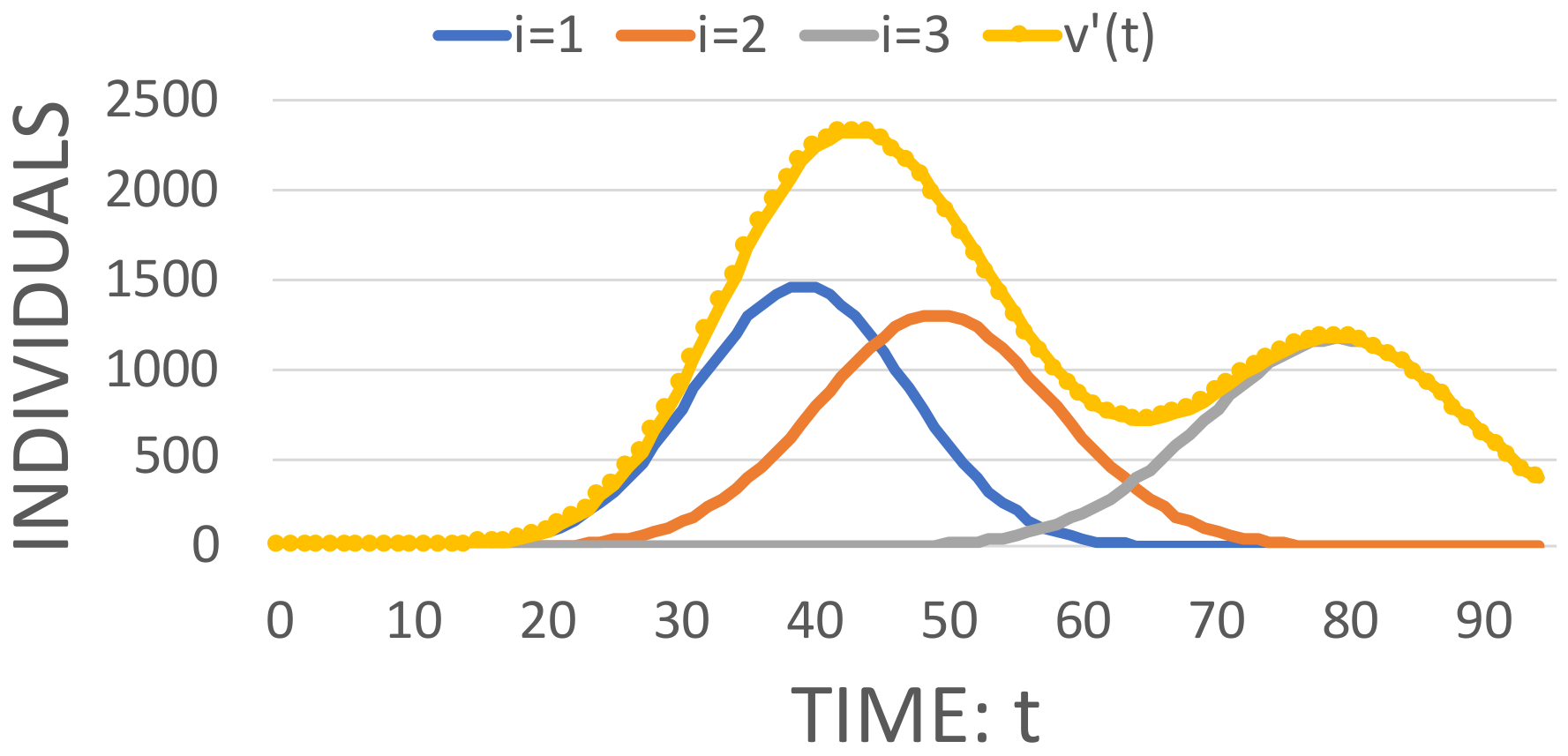
Figure 1 shows a simulation of Equation (15) using three Gaussian functions. The numerical values for the respective parameters are given in the caption.

Each Gaussian function represents the temporal evolution of an epidemic variable, $v^{\prime }$, for a distance $x_i,i=1,2,3$. The space-dependent means, ${\mu }_v\left(x_i\right)$, standard deviations, ${\sigma }_v\left(x_i\right)$, and constant parameters, $C_v^{\prime }$, characterize the sum of functions. $N_v$ is another parameter that determines the number of Gaussian components in the sum. This parameter may be regarded as the number of distances for which temporal Gaussian components of the epidemic variable are evaluated.

5. Numerical Experiments

In this section, the methodology used to compare the model performance of our proposal to the LGM, ORM, and GRM phenomenological models is explained. The evaluation strategy is based on each model’s ability to describe empirical trajectories of real epidemics. Using this methodology, we provide conclusions on which is the best model for each outbreak and type of individual.

The evaluation methodology involves the implementation of the following steps:

• Obtain real data in the time series of an epidemic outbreak.
• Select the model and provide values for initial parameters, in addition to the lower and upper bounds for final parameters.
• Estimate model parameters and their confidence intervals.
• Quantify the error of the model fit to real data.
• Compare the quality of the fits and the errors yielded by the models across all of the epidemics.

5.1. Epidemic Datasets

We used real data series that measure the temporal changes in the number of individuals. We employ a data set for six different epidemic trajectories with different temporal resolution (see

Table 1. Six real datasets used in numerical experiments. The information for each epidemic time-series data includes the name of the associated disease, the location where the outbreak occurred, temporal resolution (days, weeks), type of individual (infected, dead), date range, number of data points, and data source. ICU is Intensive Care Unit.

Dataset ID	Disease	Outbreak	Individuals	Resolution	Dates	Total Data	Source
C19InSp	COVID-19	Spain	infected	day	4/3/20–20/5/20	78	[22]
C19DeSp	COVID-19	Spain	dead	day	20/2/20–20/5/20	91	[22]
EboInSL	Ebola	Sierra Leone	infected	week	65 weeks, 2014–2016	65	[4]
ZikInCo	Zika	Colombia	infected	day	27/12/15–8/4/16	104	[14]
C19ICUSp	COVID-19	Spain	admitted-to-the-ICU	day	8/3/20–23/5/20	77	[22]
C19HDSp	COVID-19	Spain	hospital-discharge	day	8/3/20–17/5/20	71	[22]

).

5.2. Estimation of the Model Parameters

Each model, f, uses a different set of parameters, ${\theta }_f=({\theta }_1^f,\dots ,{\theta }_{m_f}^f)$. To fit the models to the data that allow us to estimate the parameters, we have employed the least-square method implemented by the $curve\_fit$ function that used the $Levenberg-Marquardt$ algorithm and is provided by the function set $optimize$ of the $SciPy$ library of $Python$. This method searches for the set of parameters that minimize an objective function that employs real data and a model function. Initial values and lower and upper bounds for the parameters were needed. For GRM, the $scipy.integrate.solve\_ivy$ Python function was used to solve the ordinary differential equation 3 to obtain the model function before the objective function is calculated.

To quantify parameter uncertainty and construct confidence intervals, we used the parametric bootstrap method [4,12,23]. The negative binomial error structures were employed to generate 200 model realizations. For the negative binomial error structures, the ratios of the variance to the mean were separately calibrated for each epidemic dataset. This was due to that each real dataset shows a different overdispersion. In the case of overdispersion, the negative binomial model gives more appropriate confidence intervals [24]. From the 200 realizations, we calculate 95% confidence intervals for model parameters to measure their uncertainties. In addition, the median values of the model parameters were obtained.

The experimental work with the overdispersed datasets also used Poisson error structures. However, and similarly to other epidemiological studies [25], we concluded that the Poisson model underestimates variability present in a dataset leading to narrower confidence intervals which more often exclude the true value. These results were not included in this paper because there are more incorrect inferences when the Poisson approach is used for model fitting than the negative binomial model.

To avoid overparameterizing our model by using a variable number of Gaussian components, we fit increasing numbers of components. Thus, we judge the improvement sequentially as is suggested in [26].

We used the following method to estimate the number of Gaussian components, $N_v$, in Equation (15) [21]: (1) Start the analysis with $N_v=1$, (2) from 200 realizations of the bootstrap method above-mentioned, a curve fitting with the median values for the epidemic variable $v^{\prime }$ is obtained, (3) calculate the respective value of the root mean square error (RMSE) using Equation (16), (4) add another Gaussian function into the analysis and repeat step (2), and (5) keep increasing the number of Gaussian functions until reaching the minimum value for the RMSE. Thus, the optimal number of components is the one providing the minimum value of the RMSE calculated for each number of Gaussian functions considered in the analysis.

The execution time of our sequential program that implements all model fits was measured using a 2012 iMac computer. It has a 2.9 GHz Intel Core i5 processor (Ivy Bridge, I5-3470S) and 8 GB 1600 MHz DDR3 memory.

5.3. Errors of the Model Fits

To compare the models, we have used the RMSE metric,

$$RMSE=\sqrt{\frac{1}{n}\sum _{i=1}^n{\left(f(t_i,{\widehat{\theta }}_f)-y_i\right)}^2}$$

(16)

where $t_i,i=1,\dots ,n$ are dates of data, ${\widehat{\theta }}_f$ is the set of parameters of the best fit model, f, and $y_i$ are the time series data for a specific epidemic outbreak. This metric was also used to obtain the $N_v$ parameter of our epidemic model whose function is given in Equation (15). For this model, the selected $N_v$ provides the lowest RMSE value. The value of this parameter also depends on the type of individual (infected, dead, etc.).

The model fits can also be evaluated by analyzing the variation of residuals, the difference between the best fit of the model and the time-series data. Some authors have used residuals to evaluate the quality of the model fit to the data [4]. The following formula that calculates the residuals for each model fit f to the data y, is used in this work to compare the mathematical models,

$$res\left(t_i\right)=f(t_i,{\widehat{\theta }}_f)-y_{i}i=1,\dots ,n$$

(17)

A random pattern in the temporal variation of the residuals suggests a good fit of the model to the data. Thus, in addition to RMSE, the mean and standard deviation of the residuals of a model fit to an epidemic dataset are also taken as performance metrics.

6. Results

Table 2. Experimental setup for each epidemic dataset.

Dataset ID	Data Fitting Method	Error Structure	Variance/Mean	Number of Model Realizations
C19InSp	curve_fit	NegativeBinomial	400	200
EboInSL	curve_fit	NegativeBinomial	20	200
ZikInCo	curve_fit	NegativeBinomial	5	200
C19DeSp	curve_fit	NegativeBinomial	40	200
C19ICUSp	curve_fit	NegativeBinomial	10	200
C19HDSp	curve_fit	NegativeBinomial	80	200

summarizes the data fitting method and error structure that we have employed for each dataset to generate many model realizations using the parametric bootstrap method described in Section 5.2. When a negative binomial error structure is assumed, this table includes the number of times the variance is higher than the mean.

6.1. Parameter Estimates with Quantified Uncertainty

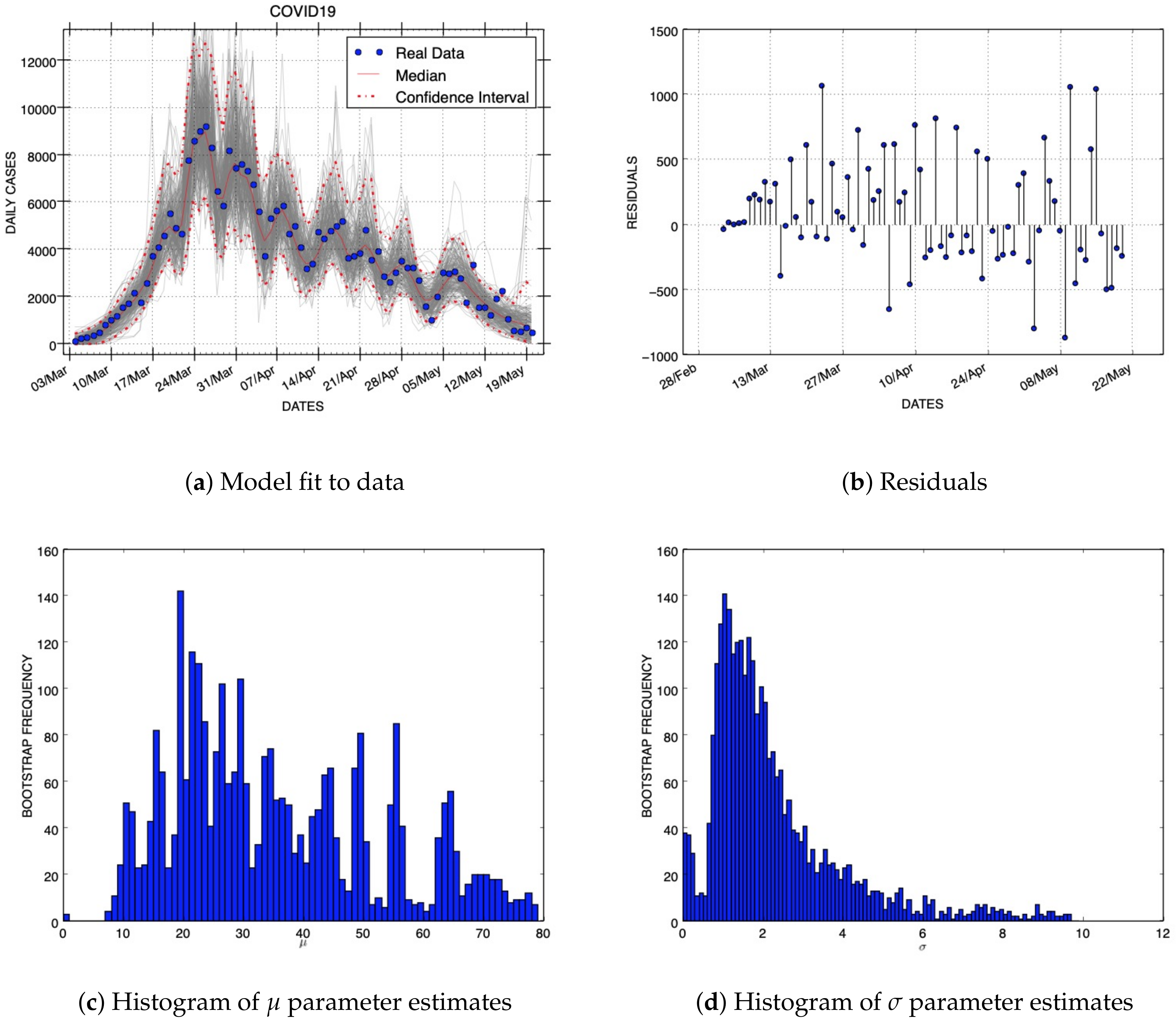
Figure 2 shows the results of our model fit, residuals, and uncertainty of two parameters using the C19InfSp COVID-19 dataset. The blue circles of the panel that shows the model fit are the daily data (y), while the solid red line corresponds to the best fit of the Gaussian model (f). The dashed red lines correspond to the 95% confidence bands around the best fit of the model to the data. The gray lines represent to the number of realizations shown in Table 2 of the epidemic curve assuming a negative binomial error structure. The blue circles of the picture that shows the residuals were obtained using Equation (17). The histograms display the empirical distributions of the parameter estimates using the above-mentioned number of bootstrap realizations.

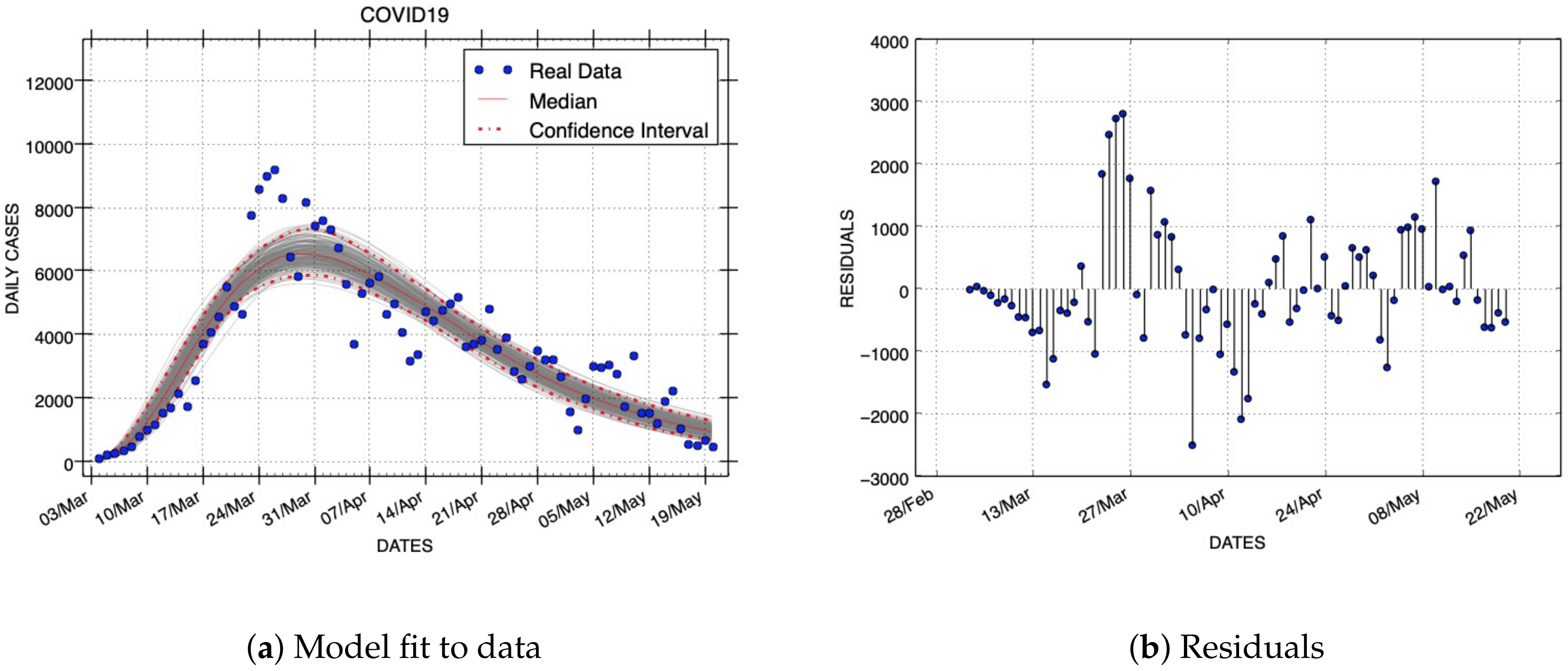
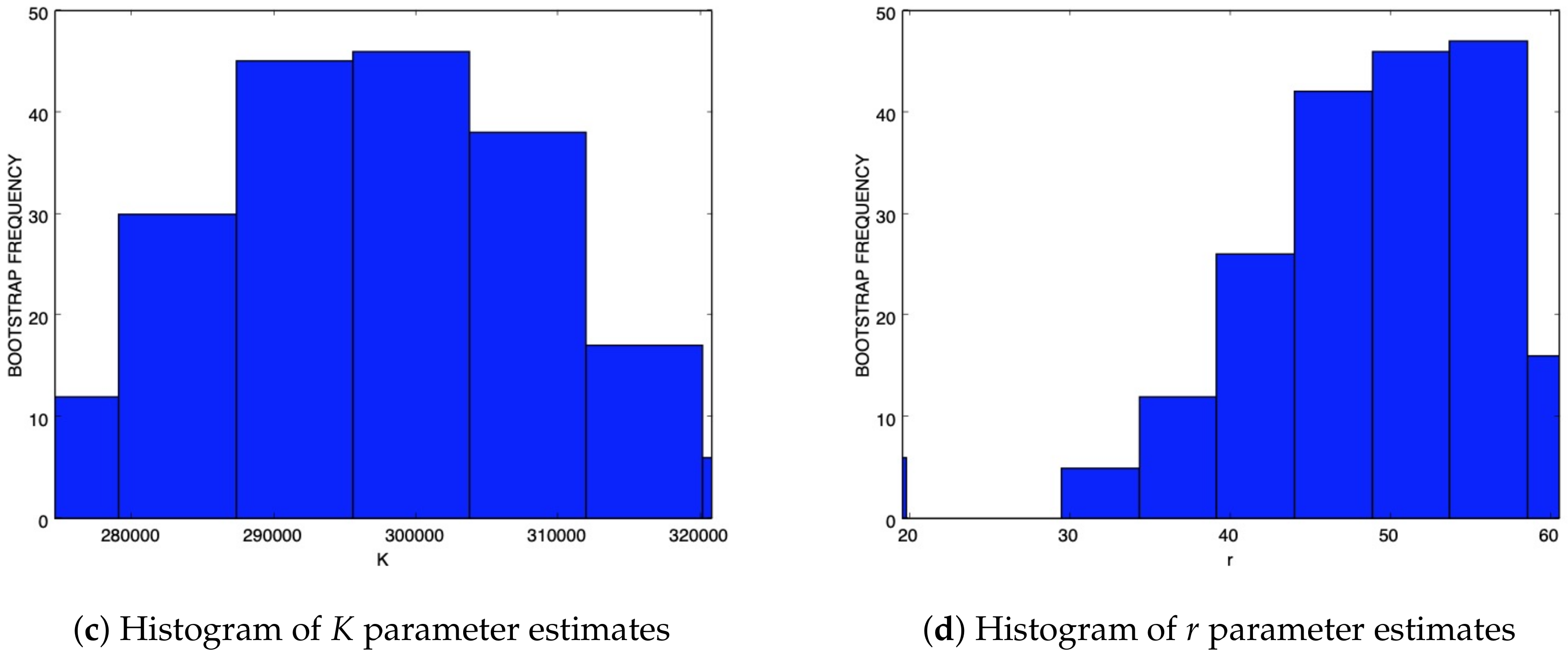
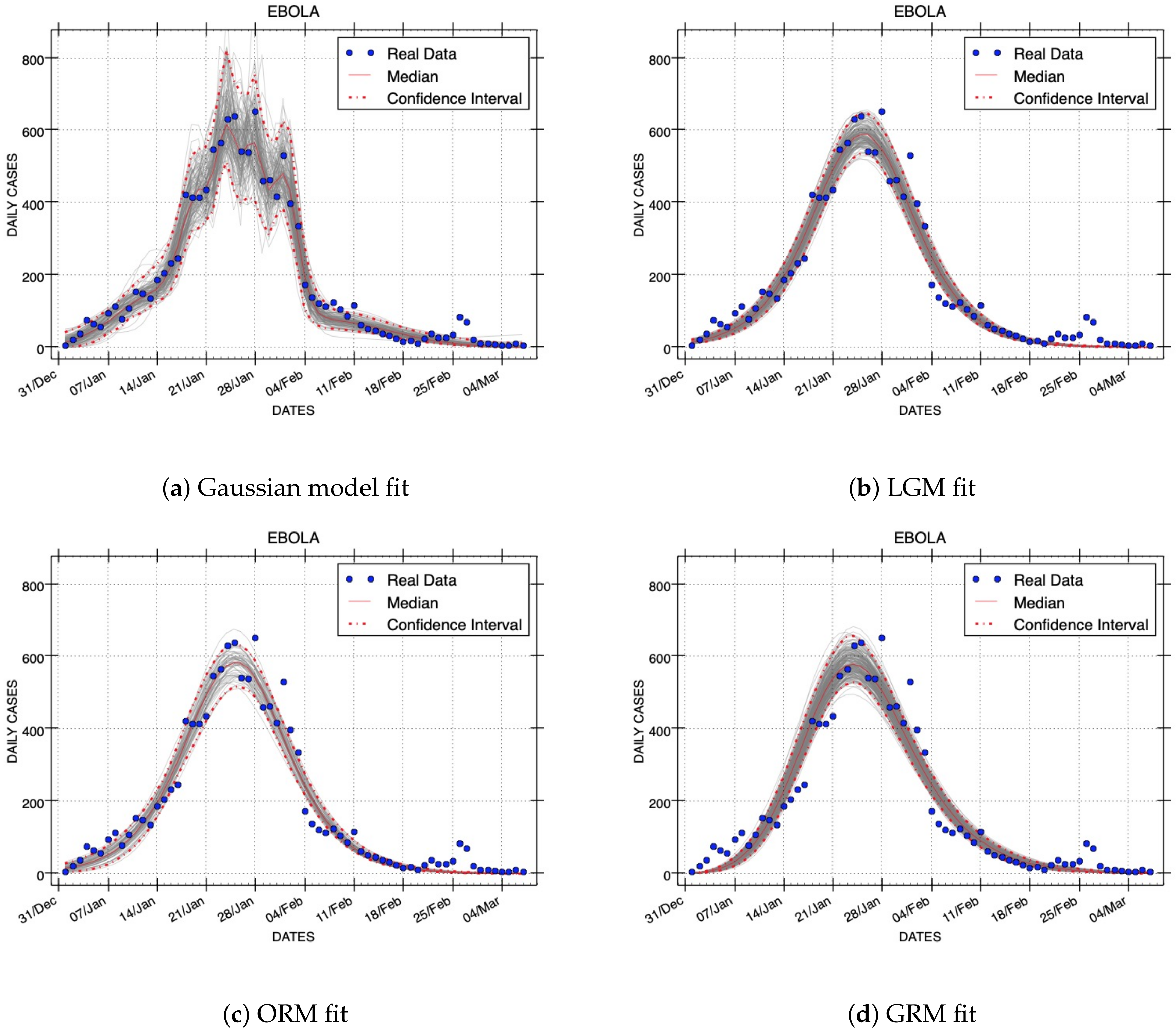
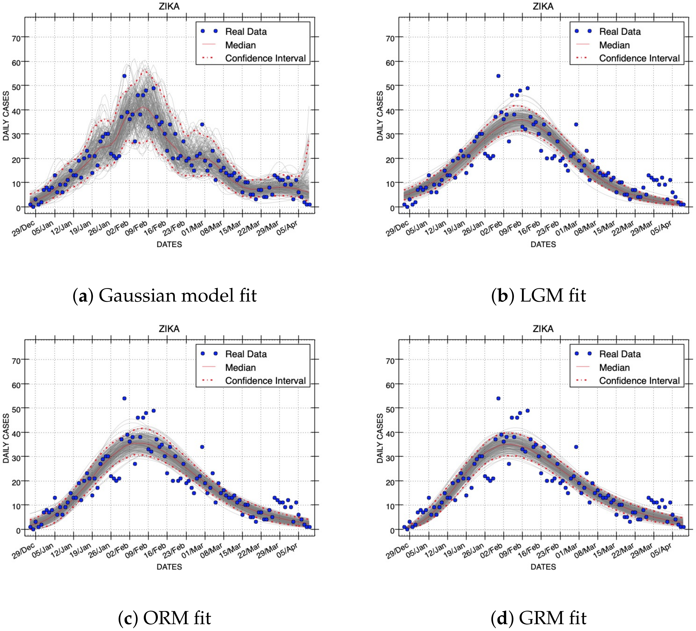
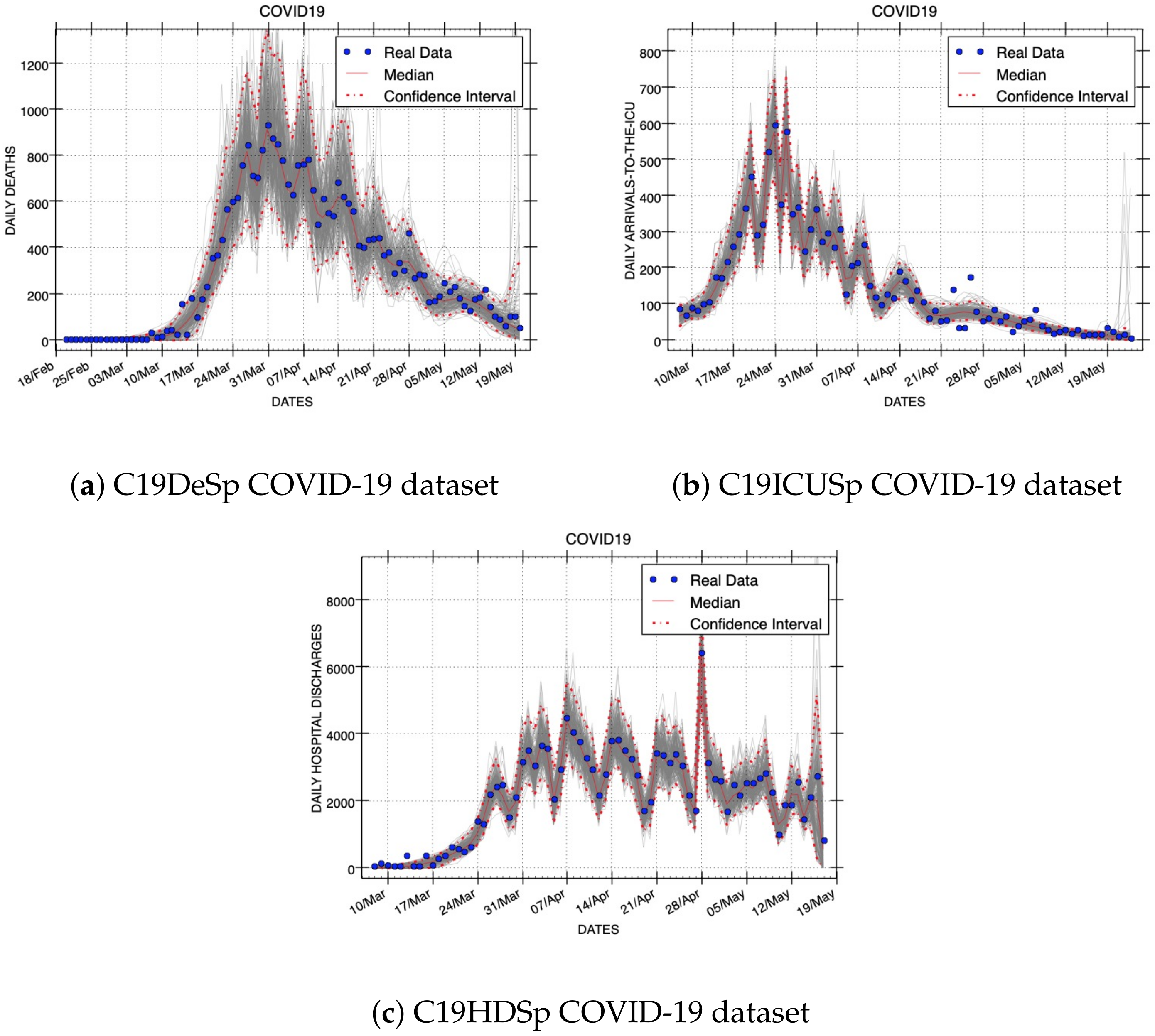
For the same dataset, Figure 3 shows the results obtained with the Generalized Richards Model. The results of all model fittings for the EboInSL Ebola and ZikInCo Zika datasets are shown in Figure 4 and Figure 5, respectively. Figure 6 shows three Gaussian model fits for variables that represent other epidemic quantities: deaths, admitted-to-the-ICU, and hospital discharges, respectively. We have not studied the curve fits of LGM, ORM, and GRM for these three epidemic variables because the models are not designed for them. The resulting quantification of parameter uncertainty around all models fits are shown in

Table 3. Parameter uncertainty of epidemic models: Gaussian (see Equation (15)), Logistic Growth Model (LGM) (see Equation (1)), Original Richards Model (ORM) (see Equation (2)), and Generalized Richards Model (GRM) (see Equation (3)).

Dataset ID	Parameter Median							Parameter 95% Confidence Interval
	Gaussian Model			LGM				Gaussian Model			LGM
	${\mathbf{N}}_{\mathbf{v}}$	${\mathbf{C}}_{\mathbf{v}}^{\prime }$	${\mathbf{\mu }}_{\mathbf{v}}$	${\mathbf{\sigma }}_{\mathbf{v}}$	r	K	${\mathbf{C}}_{\mathbf{v}}^{\prime }$			${\mathbf{\mu }}_{\mathbf{v}}$	${\mathbf{\sigma }}_{\mathbf{v}}$	r	K
C19InSp	16	$1.9·{10}^4$	34.4	1.9	$8.8·{10}^{-2}$	$3.0·{10}^5$	$1.7·{10}^4$–$2.4·{10}^4$			$10.8$–$2.1·{10}^5$	$0.2$–$1.7·{10}^4$	$7.8·{10}^{-2}$–$9.9·{10}^{-2}$	$2.7·{10}^5$–$3.3·{10}^5$
EboInSL	6	$1.9·{10}^3$	25.3	2.2	$0.21$	$1.2·{10}^4$	$1.8·{10}^3$–$2.1·{10}^4$	$11.3$–$38.0$	$1.2$–$12.1$	$0.19$–$0.22$	$1.1·{10}^4$–$1.3·{10}^4$
ZikInCo	14	$2.4·{10}^2$	72.1	11.1	$7.7·{10}^{-2}$	$1.9·{10}^3$	$1.9·{10}^2$–$3.2·{10}^2$			$3.0$–$1.0·{10}^3$	$3.0$–$1.0{10}^3$	$6.7·{10}^{-2}$–$8.8·{10}^{-2}$	$1.7·{10}^3$–$2.1·{10}^3$
C19DeSp	14	$2.1·{10}^3$	47.9	1.7	-	-	$1.8·{10}^3$–$2.3·{10}^3$			$28.8$–$90.0$	$0.6$–$14.4$	-	-
C19ICUSp	8	$1.5·{10}^3$	20.7	4.1	-	-	$1.4·{10}^3$–$1.9·{10}^3$			$0.0$–$94.4$	$1.2$–$37.6$	-	-
C19HDSp	23	$7.0·{10}^3$	42.4	1.2	-	-	$6.4·{10}^3$–$1.1·{10}^4$			$14.8$–$1.4·{10}^2$	$0.4$–$25.1$	-	-
Dataset ID	Parameter Median							Parameter 95% Confidence Interval
	ORM			GRM				ORM			GRM
	r	K	a	r	K	a	p	r	K	a	r	K	a	p
C19InSp	213.6	$2.9·{10}^5$	$3.1·{10}^{-4}$	51.8	$29.7·{10}^5$	$4.6·{10}^{-3}$	$0.89$	$0.3$–280	$2.6·{10}^5$–$3.0·{10}^5$	$2.4·{10}^{-4}$–$0.29$	$19.6$–$60.6$	$2.7·{10}^5$–$3.2·{10}^5$	$4.3·{10}^{-3}$–$6·{10}^{-3}$	$0.82$–$0.91$
EboInSL	0.21	$1.2·{10}^4$	$0.98$	0.95	$1.2·{10}^4$	$0.98$	$0.82$	$0.15$–$0.34$	$1.1·{10}^4$–$1.3·{10}^4$	$0.5$–$1.4$	$0.61$–$1.22$	$1.1·{10}^4$–$1.3·{10}^4$	$0.25$–$0.99$	$0.78$–$1.0$
ZikInCo	0.23	$1.9·{10}^3$	$0.28$	0.72	$1.9·{10}^3$	$0.66$	$0.74$	$8.4·{10}^{-2}$–$1.5·{10}^2$	$1.7·{10}^3$–$2.1·{10}^3$	$3.3·{10}^{-4}$–$0.93$	$0.46$–$1.81$	$1.7·{10}^3$–$2.1·{10}^3$	$3.6·{10}^{-3}$–$1.0$	$0.62$–$1.0$

.

6.2. RMSE Errors

The median values and 95% confidence intervals for the root mean squared errors yielded by all models and epidemic dataset can be seen in

Table 4. Median and 95% confidence interval of the RMSE errors (Equation (16)) of the best model fits to the real datasets.

Dataset ID	Median RMSE				RMSE 95% Confidence Interval
	Gaussian	LGM	ORM	GRM	Gaussian	LGM	ORM	GRM
C19InSp	783.74	1151.6	1161.12	1777.9	610.5–1021.9	922.0–1379.2	942.4–1443.2	1201.6–2691.3
EboInSL	44.67	56.11	54.32	68.32	33.41–61.13	42.2–76.2	42.3–67.4	44.0–110.4
ZikInCo	8.37	9.06	9.13	15.61	7.0–10.2	7.2–11.2	7.6–11.1	10.2–22.8
C19DeSp	79.05	-	-	-	58.1–104.3	-	-	-
C19ICUSp	29.84	-	-	-	24.5–35.6	-	-	-
C19HDSp	180.16	-	-	-	84.7–311.7	-	-	-

. Comparing the size of errors for each model and epidemic outbreak, it can be observed in this table that our Gaussian model yields the smallest median RMSE for all the datasets that register infected individuals. Concerning the logistic or Richards model that achieves the lowest median RMSE for each epidemic dataset, the Gaussian model improves the median RMSE by 31.9%, 17.8%, and 7.6% for C19InSp, EboInSL, and ZikInCo, respectively. On average, the performance improvement of the Gaussian model is 19.6%. LGM and ORM yield similar RMSE errors that are always larger than the Gaussian model and smaller than GRM (see Table 4). Furthermore, the endpoints of the 95% confidence intervals are lower than the respective endpoints provided by the other models. Therefore, we can conclude that the Gaussian model provides better model fit to the data than LGM, ORM, and GRM when the RMSE metric is used to evaluate model performance.

Now, we compare one representative graphic sample from the model fits of each model. These plots were obtained with the median values of model parameters. The comparison uses two epidemic outbreaks. Their dataset IDs are EboInSL and ZikInCo.

Figure 4 and Figure 5 show the model fits using median values for the respective parameters that correspond to the RMSE errors shown in Table 4. We can observe in these figures the quality of the fits. Note that the best fits to the data correspond to the smaller RMSE errors. The plots obtained with the Gaussian model follow more closely the epidemic dynamics than the other models studied in this work.

The width of confidence intervals can be also graphically compared. Confidence intervals are depicted in Figure 4 and Figure 5 using red dashed lines. Assuming a negative binomial error structure and the same variance to mean ratios (see Table 2), the Gaussian model includes more real data inside the width of confidence intervals than the rest of the models. This experimental evidence demonstrates that the Gaussian Epidemic Model is more flexible than LGM, ORM, and GRM to account for the variability in the data.

6.3. Residuals

In our experiments, the residuals or systematic deviations for the model fit to the data were quantified with Equation (17). Using parameter medians for each model fit and all epidemic datasets, the resulting mean and standard deviation of residuals are shown in

Table 5. Mean and standard deviation of the residuals (Equation (17)) obtained for the best fits of the epidemic models that are compared in this work. Additionally, the execution times needed by all model fittings to data are included. Time was measured in seconds (s).

Dataset ID	Mean of Residuals				Standard Deviation of Residuals				Execution Time [s]
	Gaussian	LGM	ORM	GRM	Gaussian	LGM	ORM	GRM	Gaussian	LGM	ORM	GRM
C19InSp	66.18	57.53	68.5	32.18	372.39	1349.44	1048.28	981.80	762	5	42	1472
EboInSL	5.32	5.50	6.56	0.31	27.81	40.0	39.93	51.54	255	3	36	270
ZikInCo	0.20	0.55	0.36	0.16	4.60	5.68	5.39	5.55	3945	5	48	858
C19DeSp	11.36	-	-	-	36.95	-	-	-	376	-	-	-
C19ICUSp	0.82	-	-	-	42.35	-	-	-	395	-	-	-
C19HDSp	33.43	-	-	-	203.45	-	-	-	5777	-	-	-

. In Figure 2b and b, the residuals for two model fits to COVID-19 data are displayed. Note that residuals can be positive or negative. Both figures show random patterns of the residuals that suggest that Gaussian and GRM models provide reasonably good fits. Additionally, the variances of residuals seem to be homogeneous.

The rest of the model fittings to real data studied in this work also provide random patterns of the residuals when data from all phases of epidemics are involved in the analysis of one dataset. The analysis of a determined epidemic sub-phase might indicate a systematic deviation of the model to the data, but it is outside the scope of this paper.

The standard deviation of residuals is desired to be smaller because it indicates that the data points are closer to the fitted line. Thus, smaller values of the standard deviation of residuals suggest a better model fit than larger values. Note that the standard deviations of residuals of the Gaussian model fits are always lower than the best of the logistic and Richards models by 62.1%, 30.5%, and 14.7% for C19InSp, EboInSL, and ZikInCo, respectively (see Table 5). On average, the performance improvement for these epidemic outbreaks using the residuals metric is 35.7%. Therefore, the analysis of residuals indicates that the Gaussian model is better for the epidemic datasets used in this work than the logistic and Richards models.

The basic assumptions for non-linear regression models are that the errors are random observations from a normal distribution with zero mean and constant standard deviation. Thus, the means of residuals closer to zero suggest better non-linear model fits than means that are far from zero. Note in Table 5 that the means of residuals for each model fit are similar, although GRM provides the smallest values in two from three epidemic datasets of infected individuals.

6.4. Computational Load

Each model fit needs a different computational load that causes different execution times if the same computer and software implementations are employed. The execution time of software programs may be important if they are used for real-time epidemic predictions. Thus, we have also compared the elapsed time that our programs need to fit the models to the data. Table 5 also shows the execution times of all model fittings. The interval of time needed by the programs used in this work is mainly caused by the computational load, i.e., the arithmetic operations and memory accesses. Exhaustive performance evaluation of programs for fitting the models to the data is out of the scope of this paper.

For the same dataset, LGM always needs the smallest execution time. However, this model always yields a worse fitting performance than the Gaussian model. LGM and ORM need less computational load than GRM. It is due to that the model fits use the analytical solutions of Equations (1) and (2), respectively. However, GRM repetitively requires to solve numerically Equation (3) during the searching of optimal parameters. Additionally, since the number of parameters used in LGM is smaller than ORM, the execution time is also smaller (see Table 5).

The Gaussian model is computationally costly in comparison to LGM and ORM. Comparing the software performance of the implementations of the fitting processes using Gaussian and GRM models, there is not a clear winner. Although the Gaussian model does not require to solve numerically a differential equation, the number of parameters to estimate may cause larger execution times than LGM, ORM, and GRM.

6.5. Forecasts

Mathematical models have been also proposed to predict their behaviors in the near or long terms. In this section, we compare short-term forecasts of the Gaussian model with the other three phenomenological models. The method employed to do forecasts consists of calibrating each model (f) with a given dataset ($y_i^t,i=1,\dots ,N_t$) and then, propagating the last state of the model at time t by a time horizon of $h=1,2,\dots ,N_h$: $f(t+h,{\theta }^t)$. ${\theta }^t$ is the set of parameters used in a determined forecast. RMSE was used to quantify the error associated with each model calibration. We also propagated the uncertainty of the last state at time t using the sets of parameters provided by $N_S$ bootstrap realizations: ${\theta }_i^t,i=1,\dots ,N_S$ (in this work $N_S=200)$.

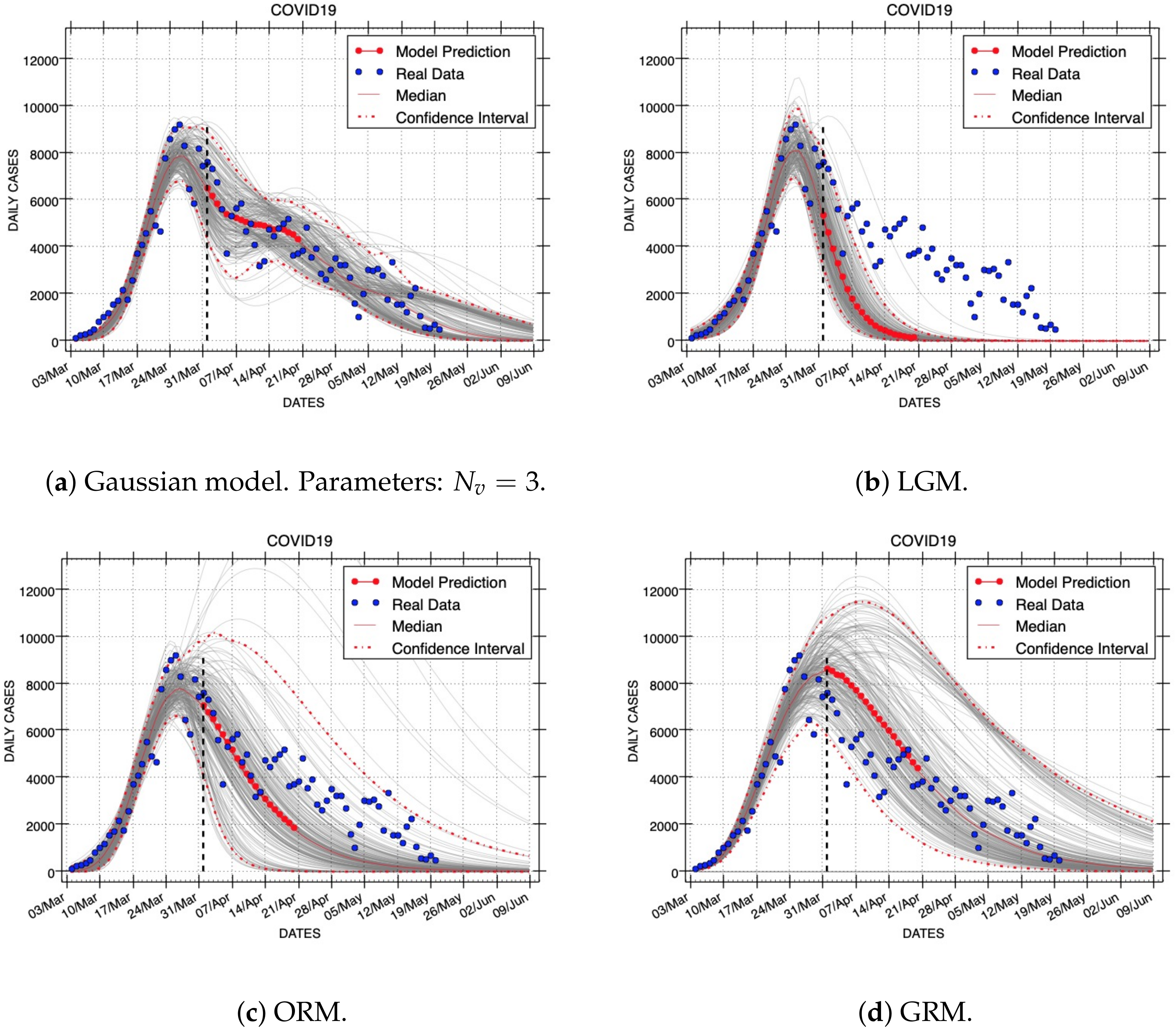
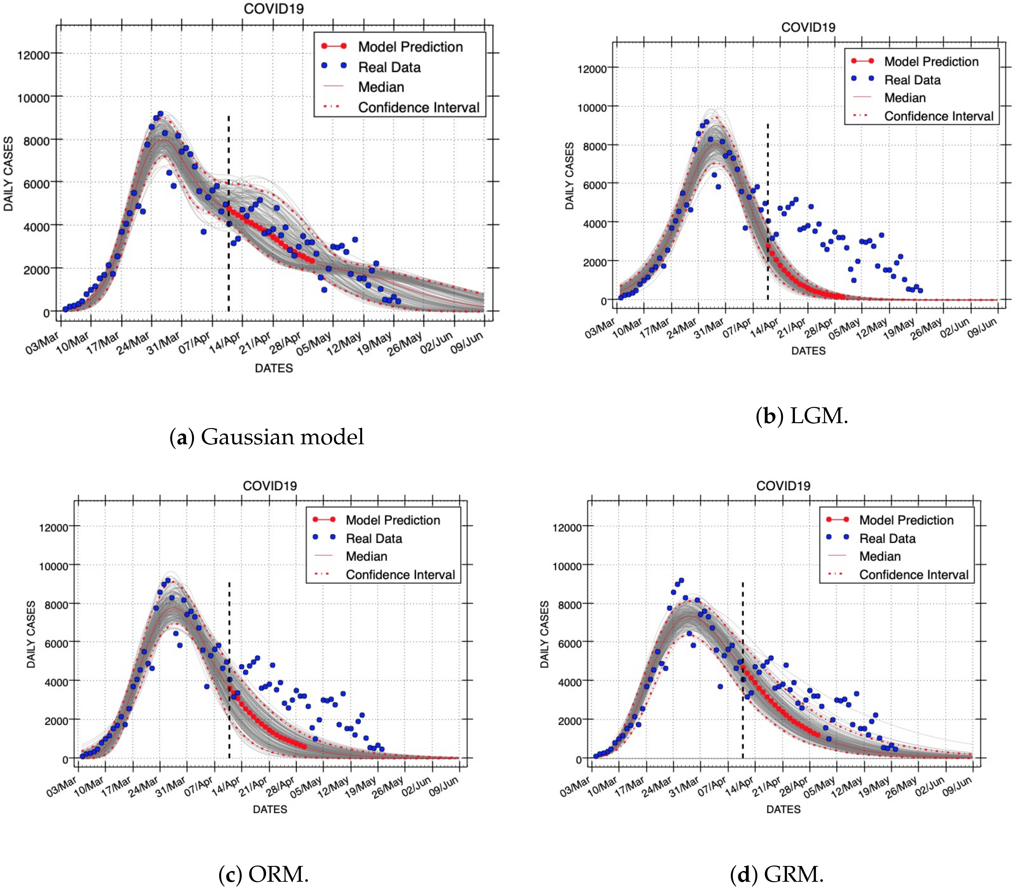
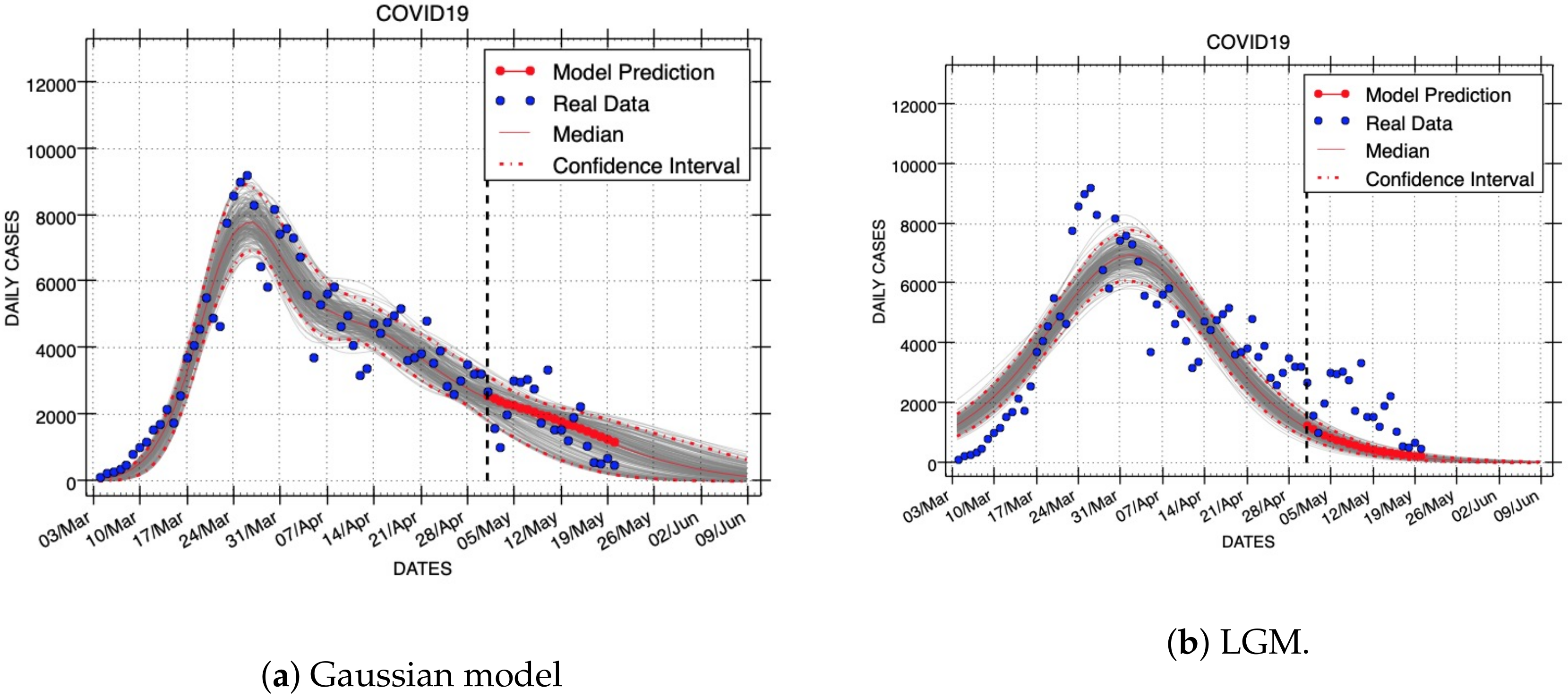
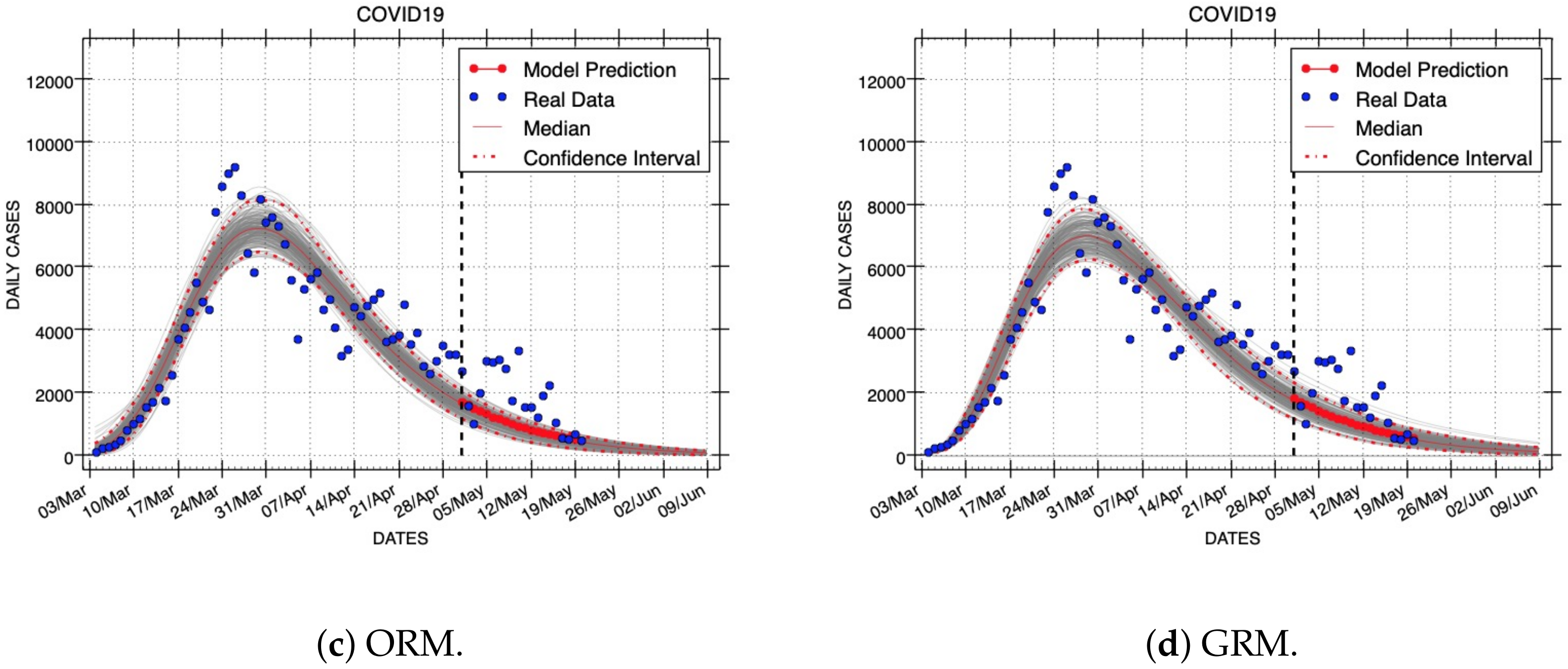
Figure 7, Figure 8 and Figure 9 show results of short- and long-term forecasts provided by all models (Gaussian, LGM, ORM, and GRM) for the COVID-19 outbreak. These figures were generated using the same real dataset called C19InSp, which contains 78 days (see Table 1). Data were separated into two periods, one for model calibration and the other for forecasting. Each figure corresponds to model fittings with the following calibration periods: $N_t=28$ (ID: Forecast-1), $N_t=38$ (ID: Forecast-2), and $N_t=58$ epidemic days (ID: Forecast-3), respectively. The forecasting period is different for each figure: $N_h=50$ (ID: Forecast-1, Figure 7), $N_h=40$ (ID: Forecast-2, Figure 8), and $N_h=20$ epidemic days (ID: Forecast-3, Figure 9), respectively. A black vertical dashed line identifies the first state after the calibration period, i.e., it separates the calibration and forecasting periods.

These forecasts include the uncertainty associated with the parameter estimates. Red dashed lines are used to show the 95% confidence interval of the variable for each time horizon h. The gray curves correspond to the ensemble of $N_S$ realizations for the respective model forecast. Red points represent the median value of the variable for the short-term forecast periods and a red line is used to denote the long-term forecasts. The blue circles denote the time series data.

The performance of models was compared using the RMSE metric of the calibration and forecasting periods. Additionally, the mean and standard deviation of residuals of forecasting periods were measured.

Table 6. Model performance measures for the three forecasting experiments shown in Figure 7, Figure 8 and Figure 9. These experiments are called Forecasts-1,2,3, respectively. The first set of three lines of the table show the root mean squared errors provided by four phenomenological models (Gaussian, LGM, ORM, GRM) for the calibration and forecasting periods. The second set of three lines show the 95% confidence intervals during the calibration and forecasting periods. The third set of three lines shows the mean and standard deviation of residuals for the forecasting intervals.

Forecast ID	Median RMSE of Calibration Interval				RMSE 95% Confidence Interval of Calibration Interval
	Gaussian	LGM	ORM	GRM	Gaussian	LGM	ORM	GRM
Forecast-1	1072.9	1047.6	1062.1	1094.9	704.0–1634.6	698.5–1570.4	688.0–1550.2	627.0–1766.4
Forecast-2	1214.4	1240.2	1221.9	1368.2	914.7–1639.8	946.1–1655.6	884.9–1639.3	907.6–2331.6
Forecast-3	1195.3	1234.2	1257.4	1672.2	958.4–1492.1	963.3–1509.9	977.0–1548.5	1088.5–2590.0
Forecast ID	Median RMSE of Forecasting Interval				RMSE 95% Confidence Interval of Forecasting Interval
	Gaussian	LGM	ORM	GRM	Gaussian	LGM	ORM	GRM
Forecast-1	1039.9	2977.7	1838.1	1576.5	796.8–1986.5	2391.0–3372.7	1259.6–3396.7	1152.3–5073.0
Forecast-2	983.1	2533.8	2013.1	1475.8	740.7–1239.1	2268.1–2768.7	1403.5–2668.2	955.4–1943.4
Forecast-3	793.1	1478.8	1143.4	1067.7	717.2–1173.0	1257.1–1660.3	920.0–1448.5	795.4–1399.8
Forecast ID	Mean of Residuals of Forecasting Interval				Standard Deviation of Residuals of Forecasting Interval
	Gaussian	LGM	ORM	GRM	Gaussian	LGM	ORM	GRM
Forecast-1	22.1	2977.7	1803.7	-310.1	783.1	1651.1	1165.5	1270.7
Forecast-2	96.2	1196.5	977.8	597.7	783.7	1530.5	1222.1	1088.0
Forecast-3	68.6	334.4	231.8	273.6	760.6	1530.5	1048.5	987.4

shows these performance metrics for the three calibration and forecast periods: Forecasts-1,2,3.

The performance for the calibration intervals depends on how much data are used to fit each model. Our Gaussian model provides better data fitting than the other three models as the calibration interval is longer (see $MedianRMSEofCalibrationInterval$ in Table 6). Note that we have used three Gaussian density functions for our forecasting experiments ($N_v=3$). This means that as the number of calibrating data increases, our Gaussian model provides better data fitting.

The performance of the Gaussian model for the forecasting periods is always better than the other three mathematical models (see $MedianRMSEofForecastingInterval$ in Table 6). The Gaussian model provides always the lowest median RMSE error. Concerning the GRM, the Gaussian model improves the median RMSE error in 34.0%, 33.4%, 25.7% for Forecasts-1,2,3, respectively; on average, the performance improvement is 31.0%. Furthermore, the endpoints of the 95% confidence intervals are also lower than the respective endpoints provided by the other models. The standard deviation of residuals of the Gaussian forecasting is lower than the best of the logistic and Richards models by 32.8%, 28.0%, 23.0% for Forecasts-1,2,3, respectively; on average, the performance improvement is in this case 27.9%.

Analyzing the residuals of forecasting intervals confirms that the Gaussian model achieves the highest performance. Our model provides always the best standard deviation of residuals for the three forecasting experiments above-mentioned. Therefore, our Gaussian model provides better forecasting performance than LGM, ORM, and GRM for the real datasets used in our experiments.

7. Conclusions and Future Work

In this paper, a new phenomenological epidemic model is presented. One of the main features of this model is the introduction of a new stochastic partial differential equation that is derived from foundations of statistical physics. This differential equation has analytical solutions that describe the spatio-temporal evolution of a Gaussian probability density function. Our proposal can be applied to several epidemic variables. In this work, we have presented results of the Gaussian model fit to data that represent the following epidemic variables: infected, deaths, admitted-to-the-ICU, and hospital-discharge.

We performed a systematic comparison of the new Gaussian model with three state-of-the-art phenomenological models for three epidemic outbreaks: COVID-19, Zika, and Ebola. This study indicates that our approach achieves better performance than the other models in describing epidemic trajectories that register infected individuals. On average, the median RMSE error of our Gaussian model is reduced by 19.6% as compared to the logistic and Richards models studied in this work. The performance of model fittings was also measured using the residuals metric. In this case, the standard deviations of residuals of the Gaussian model fittings were always lower than the best of the logistic and Richards models by, on average, 35.7%.

We have also quantified the performance of all models for generating forecasts. In the evaluation of each model fit, we employed the same parameter estimation procedure, initial solutions, and final solution bounds needed by numerical optimization methods. Using three forecasting experiments for the COVID-19 outbreak, the median RMSE error and standard deviation of residuals are improved by the performance of our model on average by 31.0% and 27.9%, respectively, as compared to the best performance of the logistic and Richards models. These quantitative results may be used as experimental evidence showing that the Gaussian Epidemic Model is more flexible than LGM, ORM, and GRM to account for the variability in the data.

For Equation (15), we have approximated the accumulated values of epidemic variables with a finite sum of Gaussian density functions. In our future research, we will quantitatively characterize the error introduced by this approximation using Approximation Theory [27]. The approximation domain is expected to be established by the epidemic data set and forecasting interval.

Additionally, the execution time of a python program needs more sequential time when our new model is used compared to the fastest of the logistic and Richards models. In future work, we will build on the programming framework to reduce the execution time of the program that implements our Gaussian model.