Abstract
In this paper, an easy-to-implement domain-type meshless method—the generalized finite difference method (GFDM)—is applied to simulate the bending behavior of functionally graded (FG) plates. Based on the first-order shear deformation theory (FSDT) and Hamilton’s principle, the governing equations and constrained boundary conditions of functionally graded plates are derived. Based on the multivariate Taylor series and the weighted moving least-squares technique, the partial derivative of the underdetermined displacement at a certain node can be represented by a linear combination of the displacements at its adjacent nodes in the GFDM implementation. A certain node of the local support domain is formed according to the rule of “the shortest distance”. The proposed GFDM provides the sparse resultant matrix, which overcomes the highly ill-conditioned resultant matrix issue encountered in most of the meshless collocation methods. In addition, the studies show that irregular distribution of structural nodes has hardly any impact on the numerical performance of the generalized finite difference method for FG plate bending behavior. The method is a truly meshless approach. The numerical accuracy and efficiency of the GFDM are firstly verified through some benchmark examples, with different shapes and constrained boundary conditions. Then, the effects of material parameters and thickness on FG plate bending behavior are numerically investigated.
1. Introduction
Functionally gradient materials (FGMs) [1] are attractive to various fields such as aerospace, machinery, civil, nuclear power, chemistry, biological medicine, and electronic information due to its good mechanical performance. The FGMs often consist of two or more materials whose volume fractions are derived from a function of position through their thickness, namely, it changes continuously along certain dimensions of the structure. Recently, Bodaghi et al. [2] applied FGMs to the design of porous femoral prostheses under normal walking load conditions and discovered that using FGMs could be better than the conventional solutions. Furthermore, the development of 4D printing technology makes FGMs more popular when fabricating metamaterials [3,4,5]. Therefore, in this study, we are committed to numerically studying the FGMs’ bending behavior. Rapid developments of numerical methods have included the application of both meshed-based methods and meshless methods to the structural analysis of mechanical problems, which have been extensively investigated in research works. The objective of meshless methods is to eliminate, at least in part, the structure of elements, as in the finite element method (FEM), by constructing the approximation entirely in terms of nodes [6,7]. The presentation of a number of meshless methods is aimed at either improving the process in the calculated performance of existing methods or developing new ones. The bending analysis of plates using different versions of meshless methods has been studied in the past few decades [8,9,10,11,12,13,14]. In 1996, the static bending problem of elastic thin plates and shells was analyzed by Belytschko using the element-free Galerkin method [15]. Subsequently, Liu et al. [16] analyzed laminated plates using the element-free Galerkin method. Batra et al. [17] applied the Petrov–Galerkin meshless method, with radial basis functions to simulate the bending behavior of FGM thick plates based on higher-order shear and the normal deformable plate theory. The axisymmetric bending of functionally graded circular plates has also been studied based on the fourth-order shear deformation theory [18]. Fu et al. studied the bending analysis of the Kirchhoff and Winkler plate using the boundary particle method [19,20].
The generalized finite difference method (GFDM) [21,22] is a relatively new localized meshless method that was developed from the classical finite difference method (FDM) [23]. A point of local support domain is formed according to the rule of “the shortest distance”. Based on the multivariate Taylor series expansion and weighted least-squares fitting, the partial derivative of the underdetermined displacement at a certain node can be represented by a linear combination of the displacements at its adjacent nodes in the GFDM implementation. Unlike the finite difference method, the GFDM eliminates the need for orthogonal grid generation and extends the FDM to a more flexible scheme. While ensuring computational accuracy, the efficiency in computations is also improved under the advantage of localization in numerical algorithms. Belytschko et al. [24] developed an alternative implementation using MLS approximation. They called their approach the element-free Galerkin (EFG) method. The use of a constrained variational principle, with a penalty function to alleviate the treatment of Dirichlet boundary conditions, has been proposed in the EFG method. Otherwise, the convenience of having no transformation to boundary conditions in mathematics is highlighted in the GFDM. For the Laplace equation in the case of different domains with essential boundary conditions and irregular clouds of points, Gavete et al. [22] summarized that the GFDM appeared to be more accurate compared to the EFG method with linear approximation. As an easy-to-implement domain-type meshless method with simple mathematics and easy programming, the GFDM has the advantage of describing physical equations and mathematics without any transformation, unlike the technology in most meshless collocation methods. Similarly, the GFDM avoids the ill-conditional dense matrix issue commonly encountered in the boundary-type meshless collocation methods. Recently, this method has been widely used to solve various scientific and engineering computing problems. In 2012, Urena et al. [25] proposed the generalized finite difference method for higher-order partial differential equations. Gu et al. [26,27] successfully applied the GFDM to engineering inverse problems. The double-diffusive natural convection in fluid-saturated porous media was studied using the generalized finite difference method [28]. The application of the generalized finite difference method to the wave and diffusion problem was also studied by Fu et al. [29,30,31].
In this paper, the generalized finite difference method is applied to analyze the plate bending behavior of functionally graded materials. Based on the first-order shear deformation theory, the generalized finite difference method was developed. Firstly, a numerical discrete model of FGM plate bending, based on the first-order shear deformation theory, is presented. The effectiveness and convergence of the proposed method are verified by solving the benchmark examples with various boundaries and shapes. The effect of functionally graded material plate bending analysis, with various gradient distributions, is numerically studied.
2. Numerical Model
Consider the FGM plate, as shown in Figure 1. The length and width of the plate are shown as and with the thickness . The components of functionally graded materials (FGMs) have a continuous gradient range, changing with spatial coordinates from one side to the other along a certain direction. The material properties , (i.e., Young’s modulus of elasticity , Poisson’s ratio , density ), changing along the thickness direction of the FGM plate and obeying the law of power function, are assumed [32].
where is the volume fraction shown in Figure 2, is the gradient index of FGMs.
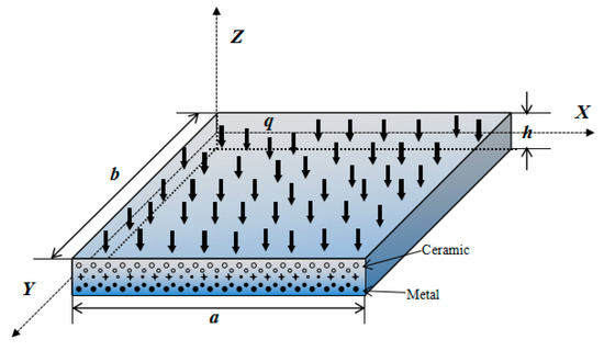
Figure 1.
Geometry of the functionally gradient material (FGM) plate.
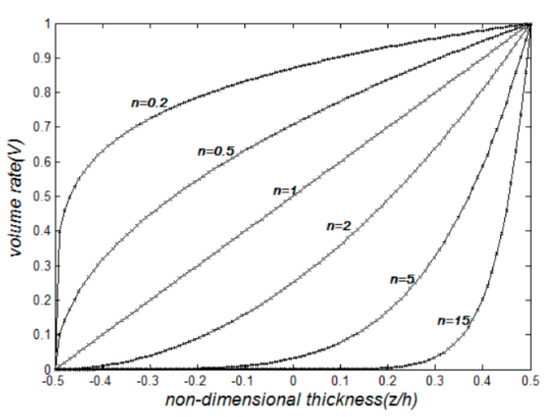
Figure 2.
Volume ratio with thickness of the FGM plate.
The first-order shear deformation theory is governed by
where is the displacement of the FGM plate, is a projection point on the middle surface of a board along the coordinates’ direction , is the corresponding rotation of the original middle surface after deformation, and is the distance to the middle plane of the FGM plate.
Based on the effect of first-order shear deformation, the strain model [33] is governed by
where
The constitutive relation for functionally graded materials is governed by
where
In Equation (7), are the tensile stiffness, coupling stiffness, and bending stiffness, respectively. are the shear stiffness for various orders. It assumed that the shear strain is constant along the thickness of the plate, using the first-order shear deformation theory. The shear correctional factor is considered due to the quadratic functional form in reality, along the thickness.
Considering the equal principle of energy between shear strain energy and shear residual strain energy, the shear correctional factor is derived by
where are the shear stiffness with shear correctional factor; the equal shear modulus is shown as .
The static differential governing equations of the FGM plate, based on the first-order shear deformation theory, are processed [34,35]
where is the internal force tensor of two-dimensional elastic mechanics, is the bending moment tensor, is the shear vector of two-dimensional elastic mechanics, and is the transverse load in a domain.
In order to obtain the unique deflection, certain constraints are imposed on the boundary of the FGM plate. Three boundary conditions are common, as follows, where is the angle between the outer normal vector and the axis vector.
Clamped boundary conditions (CBC):
Simply boundary conditions (SBC):
Free boundary conditions (FBC):
where
3. Generalized Finite Difference Method
First of all, an irregular cloud of points, , is generated in a domain. A set of points is expressed as local collocation points surrounding a central node , shown as Figure 3.
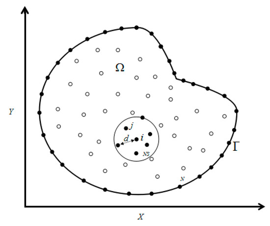
Figure 3.
Schematic diagram of collocation nodes in the generalized finite difference method (GFDM).
A differential function as a fourth-order Taylor expansion is governed by
where
In any case, the extension to other problems is obvious. We consider norm
where is the denominated weighting function [22].
The solution to the linear system may be obtained by minimizing norm using the calculus of variations.
where is the coefficient matrix formed by Euclidean distance in the appointed domain. is the matrix including explicit function value . Hence is expressed by
where ,,,...,.
Then, the process of using the generalized finite difference method will be shown at each node, according to Equations (11) and (16), and is expressed in a differential form, shown as Equation (17).
For better understanding and less writing-space, consider the first governing equation of Equation (17) as an example to describe the process. Herein, the partial derivative of the underdetermined displacement can be written in matrix forms according to Equation (16).
Based on the analyzed Euclidean distance, the coefficient at each node can be solved by the previously obtained matrix in Equation (15). In Equation (16), we shall select (nodes of star in a local region), considering a fixed radius (the same radius for all the stars of the domain) or a variable radius (the radius for each of the stars depends on their nodal distribution). That is why the sparse resultant matrix is provided in the GFDM. In the same way, all of the partial derivatives of the underdetermined displacements can be expressed as matrix forms in the GFDM. Then, the first governing equation of Equation (17) can be derived by
According to the details of the first governing equation derived by the GFDM, the other governing equations of Equation (17) are similarly derived, like Equation (18). Lastly, the complete linear equation systems of functionally graded material plates using the generalized finite difference method (GFDM) are derived, shown as Equation (19), and the displacements can be solved by the sparse linear system.
4. Numerical Results and Discussion
To illustrate the accuracy of the present approach, described in the previous sections, the static bending of homogeneous and FGM plates with different shapes is considered and analyzed. More types of the FGM plates consisting of ,, and were used throughout this work. The materials of the FGM plates are listed in Table 1. Young’s modulus and mass density are analyzed using Voigt’s rule of mixtures in Equation (1). For convenience, the boundary conditions of the FGM plates are specified as follows: free boundary condition (F), simply supported (S), or fully clamped (C). Both thin and thick plates were studied through the specified thickness-span aspect ratios in Figure 1. Normalized deflection is implemented to ignore the effect of the transverse load. Unless otherwise stated, a regular set of 12 × 12 scattered nodes was used in a square plate, shown as Figure 4b.

Table 1.
Material properties of the FGM plates used for the analysis [32].
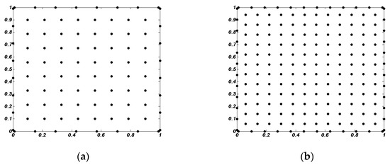
Figure 4.
Clouds (a) 8 × 8 in a domain and (b) 12 × 12 in a domain.
Consider an FGM square plate with different thickness-span aspect ratios, , subjected to a transverse uniform load that is fully simply supported (SSSS) or completely clamped supported (CCCC). Four different values of gradient index are considered for calculations in this study. Previous methods to analyze the bending of FGM plates are quoted. Table 2 reports the normalized center deflection , where the obtained results are compared with first-order shear deformation theory (FSDT)-based MK [32], FSDT-based IGA [36], and FSDT-based ES-DSG (edge-based smoothed discrete shear gap) [37]. Obviously, the numerical results solved by the present method, GFDM, agreed well with the results of the other mentioned methods.
Table 2.
Normalized center deflection of an square plate with different length-thickness ratio and gradient index under the transverse uniform load .
A further study on the effect of the nodes of star was also performed. Figure 5 depicts the convergence curves of normalized central deflection of the homogeneous plate, obtained with various values of NS (nodes of star) and with different sets of nodes. A wide range of nodes of star, from 28 to 45, was considered. As the number of nodes increases, it is observed that the situation has the same convergence to the numerical solution given by the FSDT approach [40]. Here, again, it is concluded that when NS 30, the process of convergence occurs, namely, the phenomenon of instability, because the nearly singular matrix in Equation (15) is formed with relatively fewer nodes. While 30 NS 45, it is obviously stable enough to gain the convergence curve. For appropriate computational efficiency and convergence of stability, the best result is commonly obtained with NS = 35, verified by abundant numerical calculations.
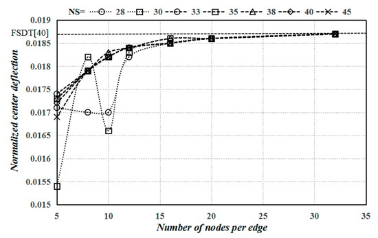
Figure 5.
Convergence curves of normalized central deflection with different values of nodes of star in a local domain in an SSSS FG plate, with a/h = 5.
The effect of the computational cost (CPU-time) using the proposed method is investigated herein. As shown in Figure 4, seven regular sets of 5 × 5, 8 × 8, 10 × 10, 12 × 12, 16 × 16, 20 × 20 and 32 × 32 nodes are used for the analysis of an SSSS homogeneous plate and a CCCC FG plate (n = 1). The intensity of scattered nodes is characterized by the distance of two neighboring nodes (), shown as Figure 3. The computational time (CPU-time) required for preprocessing and the direct full-matrix solver is evaluated, involving the definition of parameters, the partition of sets of nodes, and the implementation of the proposed method. All the tasks are performed using a personal computer with a Core-i7 CPU @ 2.5 GHz and 8 GB of RAM, based on MATLAB software. Figure 6 shows the measured CPU-time versus the nodal spacing () for different values of the nodes of star on a logarithmic scale. It is obvious that the CPU-time increases as the nodes of star increase because of an increasing local domain at each node. Similarly, Figure 7 depicts the measured CPU-time versus the nodal spacing () for a CCCC FG plate (n = 1). It is concluded that different boundary conditions and various values of gradient index have hardly any impact on the computational time. It is undisputed that the sets of nodes have a strong impact on the computational time, with 0.32 s to generate the displacement vector at 12 × 12 nodes and 2.08 s to generate the displacement vector at 32 × 32 nodes (NS = 35). Key aspects attributed to CPU-time are the efficient configuration of the point rigid body without meshing, the formation of the local support domain at a certain node, and the solver comprised of the sparse resultant matrix in the GFDM implementation. Compared to the finite element method with node-based strain smoothing [38], accuracy and effectiveness are exemplified by using the generalized finite difference method to analyze the bending of a CCCC FG plate. Based on the numerical solutions of the IGA [39] in Table 2, Figure 8 depicts the relative deviation versus increasing nodes (grids), including the finite element method with node-based strain smoothing and the proposed method. The same setting on sets of nodes and grids is used. It is clear that the relative deviation is decreasing as the sets of nodes (grids) increase, respectively generated by the two methods. It is observed that the GFDM has higher precision and faster convergence than the ES-DSG, with different values of gradient index.
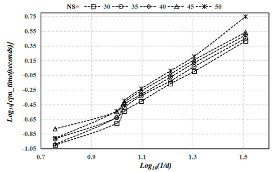
Figure 6.
The computational time (CPU-time) for solving the bending deflection of an SSSS homogeneous plate subjected to a uniform load using the present method, with different values of nodes of star in a local domain.
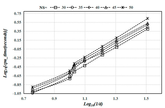
Figure 7.
The computational time (CPU-time) for solving the bending deflection of a CCCC FG plate (n = 1) subjected to a uniform load using the present method, with different values of nodes of star in a local domain.
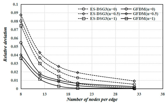
Figure 8.
The relative deviation, based on the IGA [39] in Table 2 versus 8 × 8, 12 × 12, 16 × 16, 20 × 20, and 32 × 32 nodes (grids), including the finite element method, with node-based strain smoothing [38] and the present method.
An FGM square thick plate that is fully simply supported is considered to examine the effect of different transverse loads and different gradient indices. The normalized center deflection solved by the present method is also used to compare with the results of Singha [41] and Zenkour [42]. A transverse uniform load and transverse sinusoidal load are implemented to verify the accuracy of the GFDM and analyze the bending of the FGM plate, shown in Table 3.
Table 3.
Normalized center deflection of an square thick plate with fully simply supported boundary conditions and gradient index under the transverse uniform load and the transverse sinusoidal load .
Based on the previous example and validation, the skew angle of the FGM plate was processed, shown as Table 4. An square thick plate with a fully clamped boundary condition was implemented by the present method to analyze the effect of different skew angles. As the skew angle of the FGM square plate increases, the normalized maximum deflection reduces in the figure. Obviously, the stiffness of the structure increases as the span of the structure decreases. The normalized maximum deflection of plate composed with pure ceramic is slightly less than that result of pure metal because of the super-stiff ceramic.
Table 4.
Normalized deflection of an square thick plate with fully clamped boundary conditions and different skew angles under the transverse uniform load .
The effect on various levels of irregular clouds of points in a domain is also investigated herein. The level of irregular clouds of points is characterized by a series of numbers, shown in Figure 9. Figure 10 depicts the relative deviation versus various irregular levels of sketching nodes, comparing with the original numerical solution of the present method with a regular cloud of points. In Figure 10, the results with different skew angles and gradient indices are evaluated. It is observed that the distribution of the irregular cloud of points has a slight effect on the numerical solution using the proposed method. All of the relative deviations are slightly below 1.0%. The process of numerical calculation using the generalized finite difference method has favorable stability, with various irregular clouds of points in a domain. As for the numerical analysis of structural, mechanical properties, it is absolutely essential to produce a configured model with a relatively uniform collocation of nodes (grids). The classical finite difference method needs orthogonal grids to gain equal results. The Jacobian ratio is also considered as the evaluation index of uniform grid quality in the conventional finite element method. In contrast, based on the multivariate Taylor series and the weighted moving least-squares technique, the GFDM has the advantage of obtaining stable numerical solutions from a configured model with irregular clouds of points.
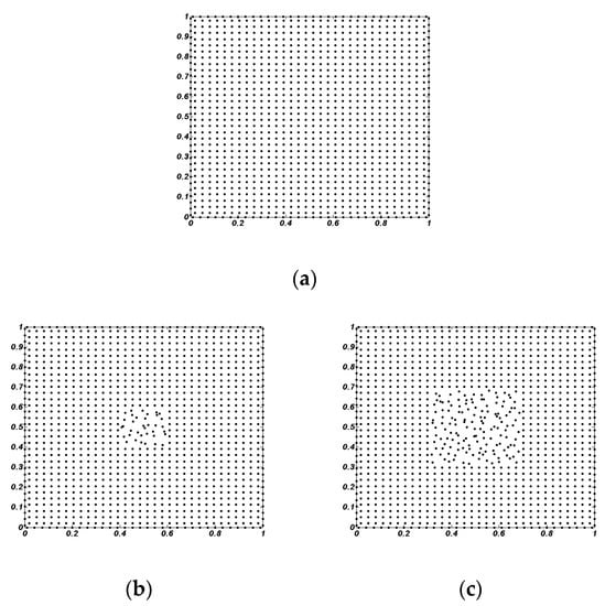
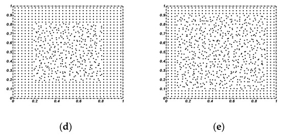
Figure 9.
The level of irregular clouds of points in a domain: (a) 0 level; (b) 1 level; (c) 2 level; (d) 3 level; and (e) 4 level.
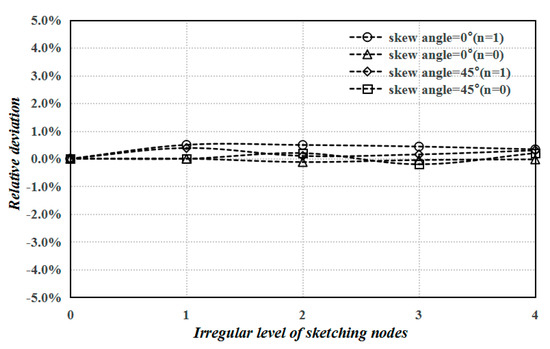
Figure 10.
The relative deviation, based on the numerical solution of the present method with a regular cloud of points versus various irregular levels of sketching nodes.
A further study for static bending of an FGM () circle thick plate with torus was performed using the proposed method. The dimensional parameters (the diameter of the circle plate, the diameter of the hole, and the gradient index ) were provided, as shown in Figure 11, Figure 12 and Figure 13. The normalized maximum deflection of FGM plate with torus and different boundary conditions under the transverse uniform load was studied, as shown in Figure 11, Figure 12 and Figure 13. The next example of static bending, with the gradient index n = 1 and different diameters of the hole, was calculated. The boundary condition of clamped support around the hole was set. The effect of the FGM circle plate with different diameters of the hole was studied under the transverse uniform load, as shown in Figure 13, Figure 14, Figure 15 and Figure 16. The normalized maximum deflection of the FGM plate with torus and different gradient indices was calculated using the present method, changing along with the diameter of the structural hole, as shown in Figure 17. It is observed that the range of size of the structural hole has a nonlinear effect on structural stiffness with different gradient indices. The normalized maximum deflection of the FGM plate with torus and different boundary conditions was analyzed, changing along with the gradient index under the transverse uniform load, as shown in Figure 18. The effect of deformation with a fully clamped pored plate is relatively minor in spite of the changing gradient index, compared with the other boundary conditions. It follows that the FGMs with various gradient indices have a substantial nonlinear effect on mechanical behavior. Some engineering significance and reference values should be provided by the proposed method, with some operating conditions.
Figure 11.
Normalized maximum deflection , with torus and fully clamped boundary conditions under a transverse uniform load .
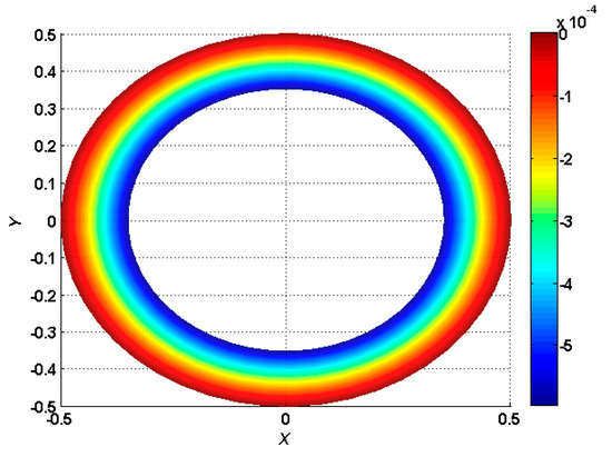
Figure 12.
Normalized maximum deflection , with torus and external clamped boundary conditions under a transverse uniform load .
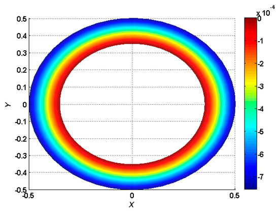
Figure 13.
Normalized maximum deflection , with torus and internal clamped boundary conditions under a transverse uniform load .
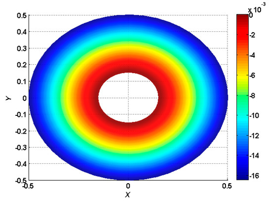
Figure 14.
Normalized maximum deflection , with torus and internal clamped boundary conditions under a transverse uniform load .
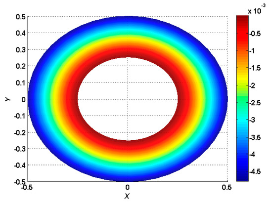
Figure 15.
Normalized maximum deflection , with torus and internal clamped boundary conditions under a transverse uniform load .
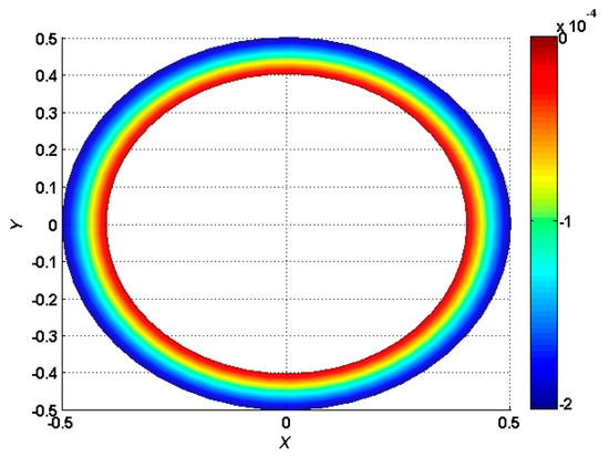
Figure 16.
Normalized maximum deflection , with torus and internal clamped boundary conditions under a transverse uniform load .
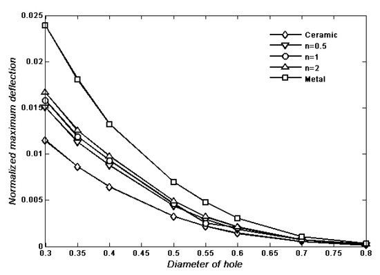
Figure 17.
Normalized maximum deflection versus diameter of the hole with internal clamped boundary conditions under a transverse uniform load .
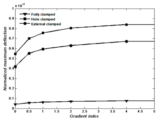
Figure 18.
Normalized maximum deflection with a hole , ranging with the gradient index under a transverse uniform load .
5. Conclusions
In this paper, a simple and easy-to-implement domain-type meshless method (GFDM) is applied to simulate the bending behavior of functionally graded material plates based on the first-order shear deformation theory. The process of using the GFDM to analyze the governing equations of the FGM plate highlights the features of simple mathematics without meshing generation and numerical integration in the GFDM. Some benchmark examples are used to verify the accuracy and availability of the method. Numerical results calculated by the generalized finite difference method in this paper agree well with those studied by other mentioned methods. The convergence and computational cost of the GFDM are investigated with different boundary conditions and various values of the gradient index. A further study shows that the GFDM has the advantage of obtaining stable numerical solutions from a configured model with irregular clouds of points. Then, the effects of material constants, geometry, and skew angles of the FGM plate are also studied by the proposed method. It is observed that, different from the isotropic materials, the FGMs with various gradient indices have a substantial nonlinear effect on mechanical behavior. The application of the meshless generalized finite difference method has been preliminarily verified to analyze FGM plate bending behavior, and the application to more complex structural analysis will be further studied in the future.
Author Contributions
The study was carried out in collaboration between all authors. Y.-D.L. completed the main part of this paper and gave examples to simulate the bending behavior of functionally graded material plates using a novel domain-type meshless method (GFDM); Z.-C.T. and Z.-J.F. corrected the main theorems and refined the manuscript. All authors have read and agreed to the published version of the manuscript.
Funding
The work described in this paper was supported by the National Science Fund of China (Grant No. 11772119, 11572111), the Fundamental Research Funds for the Central Universities (Grant No. B200202124), the Foundation for Open Project of State Key Laboratory of Mechanics and Control of Mechanical Structures (Nanjing University Of Aeronautics And Astronautics) (Grant No. MCMS-E-0519G01) and the Six Talent Peaks Project in Jiangsu Province of China (Grant No. 2019-KTHY-009).
Acknowledgments
The authors express their gratitude to the referees for their helpful suggestions.
Conflicts of Interest
The authors declare no conflict of interest. The funders had no role in the design of the study; in the collection, analyses, or interpretation of data; in the writing of the manuscript, or in the decision to publish the results.
References
- Zenkour, A.M.; Hafed, Z.S.; Radwan, A.F. Bending analysis of functionally graded nanoscale plates by using nonlocal mixed variational formula. Mathematics 2020, 8, 1162. [Google Scholar] [CrossRef]
- Chashmi, M.J.; Fathi, A.; Shirzad, M.; Jafari-Talookolaei, R.A.; Bodaghi, M.; Rabiee, S.M. Design and analysis of porous functionally graded femoral prostheses with improved stress shielding. Designs 2020, 4, 12. [Google Scholar] [CrossRef]
- Scheithauer, U.; Weingarten, S.; Johne, R.; Schwarzer, E.; Abel, J.; Richter, H.-J.; Moritz, T.; Michaelis, A. Ceramic-based 4D components: Additive manufacturing (AM) of ceramic-based functionally graded materials (FGM) by thermoplastic 3D printing (T3DP). Materials 2017, 10, 1368. [Google Scholar] [CrossRef] [PubMed]
- Bodaghi, M.; Noroozi, R.; Zolfagharian, A.; Fotouhi, M.; Norouzi, S. 4D printing self–morphing structures. Materials 2019, 12, 1353. [Google Scholar] [CrossRef] [PubMed]
- Bodaghi, M.; Damanpack, A.R.; Liao, W.-H. Adaptive metamaterials by functionally graded 4D printing. Mater. Des. 2017, 135, 26–36. [Google Scholar] [CrossRef]
- Reddy, B.; Reddy, A.; Kumar, J.; Reddy, K. Bending analysis of laminated composite plates using finite element method. Int. J. Eng. Sci. Technol. 2012, 4, 177–190. [Google Scholar] [CrossRef]
- Pham, Q.H.; Pham, T.D.; Trinh, Q.V.; Phan, D.H. Geometrically nonlinear analysis of functionally graded shells using an edge-based smoothed MITC3 (ES-MITC3) finite elements. Eng. Comput. 2020, 36, 1069–1082. [Google Scholar] [CrossRef]
- Bui, T.Q.; Nguyen, M.N. A moving Kriging interpolation-based meshfree method for free vibration analysis of Kirchhoff plates. Comput. Struct. 2011, 89, 380–394. [Google Scholar] [CrossRef]
- Bui, T.Q.; Nguyen, M.N. Eigenvalue Analysis of Thin Plate with Complicated Shapes by A Novel Mesh-free Method. Int. J. Appl. Mech. 2011, 3, 21–46. [Google Scholar] [CrossRef]
- Bui, T.Q.; Nguyen, M.N.; Zhang, C. An efficient meshfree method for vibration analysis of laminated composite plates. Comput. Mech. 2011, 48, 175–193. [Google Scholar] [CrossRef]
- Dinis, L.M.J.S.; Jorge, R.M.N.; Belinha, J. An Unconstrained Third-Order Plate Theory Applied to Functionally Graded Plates Using a Meshless Method. Mech. Adv. Mater. Struct. 2010, 17, 108–133. [Google Scholar] [CrossRef]
- Wu, C.-P.; Yang, S.-W.; Wang, Y.-M.; Hu, H.-T. A meshless collocation method for the plane problems of functionally graded material beams and plates using the DRK interpolation. Mech. Res. Commun. 2011, 38, 471–476. [Google Scholar] [CrossRef]
- Zhu, P.; Liew, K.M. Free vibration analysis of moderately thick functionally graded plates by local Kriging meshless method. Compos. Struct. 2011, 93, 2925–2944. [Google Scholar] [CrossRef]
- Zhou, H.; Qin, G.; Wang, Z. Heat conduction analysis for irregular functionally graded material geometries using the meshless weighted least-square method with temperature-dependent material properties. Numer. Heat Transf. Part B Fundam. 2019, 75, 1–13. [Google Scholar] [CrossRef]
- Krysl, P.; Belytschko, T. Analysis of thin plates by the element-free Galerkin method. Comput. Mech. 1995, 17, 26–35. [Google Scholar] [CrossRef]
- Liu, G.R.; Chen, X.L.; Reddy, J.N. Buckling of Symmetrically Laminated Composite Plates Using the Element-free Galerkin Method. Int. J. Struct. Stab. Dyn. 2002, 2, 281–294. [Google Scholar] [CrossRef]
- Gilhooley, D.F.; Batra, R.C.; Xiao, J.R. Analysis of thick functionally graded plates by using higher-order shear and normal deformable plate theory and MLPG method with radius basis functions. Compos. Part B 2008, 39, 414–427. [Google Scholar] [CrossRef]
- Sahraee, S.; Saidi, A.R. Axisymmetric bending analysis of thick functionally graded circular plates using fourth-order shear deformation theory. Eur. J. Mech. A/Solids 2009, 28, 974–984. [Google Scholar] [CrossRef]
- Fu, Z.-J.; Chen, W. A truly boundary-only meshfree method applied to Kirchhoff plate bending problem. Adv. Appl. Math. Mech. 2009, 1, 341–352. [Google Scholar]
- Fu, Z.-J.; Chen, W.; Yang, W. Winkler plate bending problems by a truly boundary-only boundary particle method. Comput. Mech. 2009, 44, 757–763. [Google Scholar] [CrossRef]
- Benito, J.J.; Urena, F.; Gavete, L. Influence of several factors in the generalized finite difference method. Appl. Math. Model. 2001, 25, 1039–1053. [Google Scholar] [CrossRef]
- Gavete, L.; Gavete, M.L.; Benito, J.J. Improvements of generalized finite difference method and comparison with other meshless method. Appl. Math. Model. 2003, 27, 831–847. [Google Scholar] [CrossRef]
- Mitchell, A.R.; Griffiths, D.F. The Finite Difference Method in Partial Differential Equations; John Wiley: Hoboken, NJ, USA, 1980. [Google Scholar]
- Belytschko, T.; Lu, Y.-Y.; Gu, L. Element-free Galerkin methods. Int. J. Numer. Meth. Eng. 1994, 37, 229–256. [Google Scholar] [CrossRef]
- Ureña, F.; Salete, E.; Benito, J.J. Solving third- and fourth-order partial differential equations using GFDM: Application to solve problems of plates. Comput. Mech. 2012, 89, 366–376. [Google Scholar] [CrossRef]
- Gu, Y.; Wang, L.; Chen, W. Application of the meshless generalized finite difference method to inverse heat source problems. Int. J. Heat Mass Transf. 2017, 108, 721–729. [Google Scholar] [CrossRef]
- Li, P.-W.; Fu, Z.-J.; Gu, Y. The generalized finite difference method for the inverse Cauchy problem in two-dimensional isotropic linear elasticity. Int. J. Solids Struct. 2019, 174, 69–84. [Google Scholar] [CrossRef]
- Li, P.-W.; Chen, W.; Fu, Z.-J. Generalized finite difference method for solving the double-diffusive natural convection in fluid-saturated porous media. Eng. Anal. Bound. Elem. 2018, 95, 175–186. [Google Scholar] [CrossRef]
- Fu, Z.-J.; Xie, Z.-Y.; Ji, S.-Y. Meshless generalized finite difference method for water wave interactions with multiple-bottom-seated-cylinder-array structures. Ocean Eng. 2020, 195, 106736. [Google Scholar] [CrossRef]
- Fu, Z.-J.; Tang, Z.-C.; Zhao, H.-T. Numerical solutions of the coupled unsteady nonlinear convection-diffusion equations based on generalized finite difference method. Eur. Phys. J. Plus 2019, 134, 134. [Google Scholar] [CrossRef]
- Li, P.-W.; Fan, C.-M. Generalized finite difference method for two-dimensional shallow water equations. Eng. Anal. Bound. Elem. 2017, 80, 58–71. [Google Scholar] [CrossRef]
- Vua, T.V.; Nguyenb, N.H.; Khosravifardc, A. A simple FSDT-based meshfree method for analysis of functionally graded plates. Eng. Anal. Bound. Elem. 2017, 79, 1–12. [Google Scholar] [CrossRef]
- Yu, T.T.; Yin, S.H.; Tinh, Q.B. A simple FSDT-based isogeometric analysis for geometrically nonlinear analysis of functionally graded plates. Finite Elem. Anal. Des. 2015, 96, 1–10. [Google Scholar] [CrossRef]
- Mantari, J.L.; Granados, E.V. An original FSDT to study advanced composites on elastic foundation. Thin-Walled Struct. 2016, 107, 80–89. [Google Scholar] [CrossRef]
- Mantari, J.L.; Granados, E.V. A refined FSDT for the static analysis of functionally graded sandwich plates. Thin-Walled Struct. 2015, 90, 150–158. [Google Scholar] [CrossRef]
- Yin, S.H.; Jack, S.H.; Yu, T.T. Isogeometric locking-free plate element: A simple first order shear deformation theory for functionally graded plates. Compos. Struct. 2014, 118, 121–138. [Google Scholar] [CrossRef]
- Nguyen, X.H.; Tran, L.V.; Nguyen, T.T. Analysis of functionally graded plates using an edge-based smoothed finite element method. Compos. Struct. 2011, 93, 3019–3039. [Google Scholar] [CrossRef]
- Nguyen, X.H.; Tran, L.V.; Thai, H. Analysis of functionally graded plates by an efficient finite element method with node-based strain smoothing. Thin Walled Struct. 2012, 54, 1–18. [Google Scholar] [CrossRef]
- Valizadeh, N.; Natarajan, S.; Gonzalez-Estrada, O.A.; Rabczuk, T.; Bui, T.Q.; Bordas, S.P.A. NURBS-based finite element analysis of functionally graded plates: Static bending, vibration, buckling and flutter. Compos. Struct. 2013, 99, 309–326. [Google Scholar] [CrossRef]
- Reddy, J.N. Analysis of functionally graded plates. Int. J. Numer. Methods Eng. 2000, 47, 663–684. [Google Scholar] [CrossRef]
- Singha, M.K.; Prakash, T.; Ganapathi, M. Finite element analysis of functionally graded plates under transverse load. Finite Elem. Anal. Des. 2011, 47, 453–460. [Google Scholar] [CrossRef]
- Zenkour, A.M. Generalized shear deformation theory for bending analysis of functionally graded plates. Appl. Math. Model. 2006, 30, 67–84. [Google Scholar] [CrossRef]


Sample Availability: The datasets analyzed during the current study are available from the corresponding author and the first author upon reasonable request. | |
Publisher’s Note: MDPI stays neutral with regard to jurisdictional claims in published maps and institutional affiliations. |
© 2020 by the authors. Licensee MDPI, Basel, Switzerland. This article is an open access article distributed under the terms and conditions of the Creative Commons Attribution (CC BY) license (http://creativecommons.org/licenses/by/4.0/).