Article

Extending Fuzzy Cognitive Maps with Tensor-Based Distance Metrics

by
Georgios Drakopoulos
1,*,
Andreas Kanavos
2,
Phivos Mylonas
1 and
Panagiotis Pintelas
3
1
Humanistic and Social Informatics Lab, Department of Informatics, Ionian University, 49100 Kerkyra, Greece
2
Computer Engineering and Informatics Department, University of Patras, 26504 Patras, Greece
3
Department of Mathematics, University of Patras, 26504 Patras, Greece
*
Author to whom correspondence should be addressed.
Mathematics 2020, 8(11), 1898; https://doi.org/10.3390/math8111898
Submission received: 30 September 2020 / Revised: 21 October 2020 / Accepted: 26 October 2020 / Published: 31 October 2020
(This article belongs to the Special Issue Applications of Fuzzy Optimization and Fuzzy Decision Making)

Abstract

:
Cognitive maps are high level representations of the key topological attributes of real or abstract spatial environments progressively built by a sequence of noisy observations. Currently such maps play a crucial role in cognitive sciences as it is believed this is how clusters of dedicated neurons at hippocampus construct internal representations. The latter include physical space and, perhaps more interestingly, abstract fields comprising of interconnected notions such as natural languages. In deep learning cognitive graphs are effective tools for simultaneous dimensionality reduction and visualization with applications among others to edge prediction, ontology alignment, and transfer learning. Fuzzy cognitive graphs have been proposed for representing maps with incomplete knowledge or errors caused by noisy or insufficient observations. The primary contribution of this article is the construction of cognitive map for the sixteen Myers-Briggs personality types with a tensor distance metric. The latter combines two categories of natural language attributes extracted from the namesake Kaggle dataset. To the best of our knowledge linguistic attributes are separated in categories. Moreover, a fuzzy variant of this map is also proposed where a certain personality may be assigned to up to two types with equal probability. The two maps were evaluated based on their topological properties, on their clustering quality, and on how well they fared against the dataset ground truth. The results indicate a superior performance of both maps with the fuzzy variant being better. Based on the findings recommendations are given for engineers and practitioners.

1. Introduction

Self organizing maps (SOMs) or cognitive maps constitute a class of neural network grids introduced in Reference [1]. In these grids neuron topology is closely related to their functionality. Moreover, the unsupervised training is patterned after a modified Hebbian rule [2]. These two fundamental properties allow SOMs to approximate the shape of a high dimensional manifold, typically represented as a set of selected data points, and subsequently to construct a lower dimensional and continuous topological map thereof. The latter provides an indirect yet efficient clustering of the data points presented to the SOM during the training process. In turn, that makes SOMs important components in many data mining pipelines in dimensionality reduction, clustering, or visualization roles.
Human character dynamics are the focus of many research fields including psychology, sociology, and cognitive sciences. The Myers-Briggs Type Indicator (MBTI) is among the most well-known classifictions of human personality according to four binary fundamental factors, resulting in a total of sixteen possible personality types [3]. Understanding the psychological dynamics of the individual members of a group is instrumental in minimizing or even avoiding non-productive and time consuming frictions, while at the same time maximizing the group potential through efficient task delegation, unperturbed and unambiguous communication, and effective conflict resolution. These skills are crucial among other cases during the formation of startups, even more so when an accelerator or an incubator are involved, in assemblying workgroups for accomplishing specific missions, or during mentorship assignments [4]. These cases are indicative of the potential of such methods.
Despite their increasing significance across a number of fields, the rapid evolution of natural language processing (NLP) algorithms for estimating human emotional states [5,6], and the development of sophisticated image processing algorithms for the identification of a wide spectrum of cognitive tasks [7,8], there are still few algorithms for addressing the topic of inferring personality dynamics from text as reported in Reference [9]. Additionally, the number of applications based on tensor metrics are still few, which is the principal motivation of this work.
The primary research objective of this article is twofold. First, a multilinear weighted function is used is the construction of the topological map as the data point distance metric. Tensors naturally capture higher order interactions between explanatory variables, in this particular case the fundamental personality traits of the MBTI model. Second, each data point is represented as a matrix and not as a vector, which is currently the customary approach. This adds flexibility in at least two ways, as not only inherently two-dimensional objects can be naturally represented but also one-dimensional objects can have simultaneously more than one representations, which can be applied in cases where object representations can be selected adaptively including aspect mining and multilevel clustering. The tensor-based metric and the matrix representations are naturally combined to yield an SOM algorithm operating on two-dimensional representations of personality traits indirectly represented as text attributes. The latter are extracted from short texts from the Kaggle Myers-Briggs dataset. In addition to the main SOM algorithm, a fuzzy one is developed where membership to at most two clusters can be possible, provided that a given data point is close enough to both.
The remaining of this article is structured as follows. In Section 2 the recent scientific literature regarding tensor distance metrics, cognitive maps, and computational cognitive science is briefly reviewed. Section 3 describes the main points behind the MBTI theory. The SOM architecture is the focus of Section 4. Section 5 discusses the attributes extracted from the dataset, the proposed tensor distance metric, and the results of the experiments. Section 6 concludes this work by recapitulating the findings as well as by exploring future research directions. Tensors are represented with capital calligraphic letters, matrices with boldface capital letters, vectors with boldface lowercase letters, and scalars with lowercase letters. When a function requires parameters, they are placed after the arguments following a semicolon. Technical acronyms are explained the first time they are encountered in text. Finally, the notation of this article is summarized in Table 1.

2. Previous Work

Cognitive maps or self organizing maps constitute a special class of neural networks which are trained in an unsupervised manner in order to form a low dimensional representation of a higher dimensional manifold with the added property that important topological relationships are maintained [1]. This map is progressively constructed by updating the neuron synaptic weights through a modified Hebbian rule, which eliminates the need for gradient based training methods [10]. Their application to clustering objects in very large databases is thoroughly explored in Reference [11]. Fuzzy  cognitive maps are SOMs where clusters are allowed to overlap [12]. Their properties are examined in Reference [13]. Learning the rules of a fuzzy cognitive map can be done through genetic algorithms [14,15], optimization algorithms [16,17], or compressed sensing [18]. SOMs have been applied to clustering massive document collections [19], functional magnetic resonance images (fMRI) based on attributes extracted from the discrete cosine transform (DCT) [20], prediction of distributed denial of service (DDoS) attacks in software defined networks (SDN) [21], factory interdependencies for Industry 4.0 settings [22], task  pools for autonomous vehicles [23], and the drivers behind digital innovation [24]. Moreover SOMs have been employed for a hierarchical clustering scheme for discovering latent gene expression patterns  [25] and gene regulatory networks [26]. Given that the trained fuzzy cognitive maps can be represented as a fuzzy graph, clustering can be performed by fuzzy community discovery algorithms [27,28,29]. In Reference [30] fuzzy graphs have been used in a technique for estimating the number of clusters and their respective centroids. C-means fuzzy clustering has been applied to epistasis analysis [31] and image segmentation [32]. An extensive review for software about SOMs is given in Reference [33].
Tensor algebra is the next evolutionary step in linear algebra since it deals primarily with the simultaneous coupling of three or more vector spaces or with vectors of three or more dimensions [34]. Also, tensors can be used in the identification of non-linear systems [35,36,37]. Tensors and their factorizations have a wide array of applications to various engineering fields. Computationally feasible tensor decompositions are proposed in Reference [38], whereas other applications to machine learning (ML) are the focus of References [39,40,41]. In Reference [42] a third order tensor represents spatiosocial Twitter data about the Grand Duchy of Luxembourg and is clustered by a genetic algorithm to yield coherent districts both geographically and linguistically. Tensor stack networks (TSNs) are clusters of feedforward neural networks (FFNNs) which can learn not only from their own errors but also from those of other networks in the cluster [43]. TSNs have been applied to large vocabulary speech recognition [44] and graph resiliency assessment [45]. Tensor distance metrics have numerous applications across diverse fields including gene expression [46], dimensionality reduction [47], and face recognition [48].
Distributed processing systems such as Apache Spark play an increasingly important role in data mining (DM) and ML pipelines [49]. In Reference [50] the singular value decomposition (SVD) performs attribute transformation and selection and boosts the performance of various Spark MLlib classifiers in Kaggle datasets. A similar role is played by higher order tensor factorizations [51]. Julia is a high level programming language primarily intended for intense data management and scientific computing applications [52]. Although interpreted, it offers high performance [53] as it is based on the low level virtual machine (LLVM) infrastructure engine [54]. The capabilities and the respective performance of the various ML models of Julia are described in Reference [55] especially over massive graphics processing unit (GPU) arrays [56]. A numerical optimization package for Julia is described in Reference [57], methods for parameter estimation for partial differential equations (PDEs) are discussed in Reference [58], while the potential of a package for the simulation of quantum systems is explained in Reference [59]. Recently a package for seismic inversion was introduced [60].
Emotions are drivers of human actions as well as major components of human personality. The Myers-Briggs type indicator (MBTI) as explained among others in Reference [3] and Reference [61] has been invented in order to create a methodological framework for quantitative personality analysis [62]. This has been used in applications such as brand loyalty [63]. Also taking into account the MBTI and their interactions can lead to significant improvements in teaching [64]. In contrast to emotion models such as Plutchick’s emotion wheel [65] or the universal emotion or big five theory proposed by Eckman in Reference [66], frameworks like MBTI offer a more general view of human personality and allow the analysis of interaction between two or more persons. The connection between cognitive functions and personality type is explored in Reference [4]. An overview of the MBTI typology is given among others in Reference [67]. Finally, human emotional state can be estimated in a number of ways. Among the most significant emotional indicators is speech, which is relatively easy to capture and process since one dimensional signal processing methodologies are used [68]. Other emotional state indicators include gait [69], facial cues [70], or a combination thereof [71]. Alternatively, human emotional state can be estimated by brain imaging techniques [72].
The blueprints of a specialized cognitive system aiming at the reconstruction of events and scenes from memory are given in Reference [73]. The role of augmented- (AR) and virtual reality (VR) for cognitive training is investigated in Reference [74]. The principles and properties of cognitive tools are the focus of  Reference [75]. A more extensive approach including predictions for future cognitive systems is that of Reference [76]. Brain-computer interface (BCI) collect biosignals related to brain activity [77]. A detailed review of BCI signaling is given in Reference [78]. Convolutional neural network (CNN) architectures in Reference [79] are used to extract temporal information about the brain through BCIs, while age and gender classification with BCI is proposed in Reference [80].

3. Myers-Briggs Type Indicator

The MBTI taxonomy [3] establishes a framework for classifying the personality of an individual along the lines of the theory developed earlier by the pioneering psychologist Karl Jung [67]. It is often now routinely employed by human resources (HR) deparments around the globe in order to determine ways to maximize total employee engagement as well as to identify possible friction points arising by different viewpoints and approach to problem solving. At the core of the taxonomy are sixteen archetypal personalities with unique traits. Each such personality type is derived by evaluating the following four fundamental criteria [4]:
  • Approach to socialization: Introvert (I) vs Extrovert (E). As the name of this variable suggests, it denotes the degree a person is open to others. Introverts tend to work mentally in isolation and rely on indirect cues from others. On the contrary, extroverts share their thoughts frequently with others and ask for explicit feedback.
  • Approach to information gathering: Sensing (S) vs Intuition (N). Persons who frequently resort to sensory related functions observe the outside world, whether the physical or social environment, in order to collect information about open problems or improve situational awareness belong to the S group. On the other hand, persons labeled as N rely on a less concrete form of information representation for reaching insight.
  • Approach to decision making: Thinking (T) vs Feeling (F). This variable indicates the primary means by which an individual makes a decision. This may be rational thinking with clearly outlined processes, perhaps in the form of corporate policies of formal problem solving methods such as 5W or TRIZ, or a more abstract and empathy oriented way based on external influences and the emotional implications of past decisions.
  • Approach to lifestyle: Judging (J) vs Perceiving (P). This psychological function pertains to how a lifestyle is led. Perceiving persons show more understanding to other lifestyles and may not object to open ended evolution processes over a long amount of time. On the contrary, judging persons tend to close open matters as soon as possible and are more likely to apply old solutions to new problems.
As each of the above variables has two possible values, there is a total of sixteen possible personality types in the MBTI model as mentioned earlier. These are listed in Table 2. Each of these personality types is assigned a four-letter acronym which is formed by the corresponding predominant trait of that character type with respect to each of the four basic variables.
The above personality types are not equally encountered. On the contrary, a few types are more frequently encountered than others. The most common personality type reported is ISFJ with corresponds to 13.8 % of the US population [3]. This corresponds to roughly twice the expected frequency of 1 / 16 6.25 % . On the other hand, the less common MBTI type encountered is INTJ with a frequency of 1.5 % [64]. Among the reasons explaining this variance are educational system, peer pressure, and adaptation to urban life and its associated socioeconomic conditions. As a sidenote, it is worth mentioning that emotions are not noise in the system but rather complex motivational mechanisms whose evolution has been driven, partly at least, by a combination of factors such as the need for immediate action and cultural norms.

4. Cognitive Maps

Structurally, an SOM is a grid where each point is a neuron u k with adjustable synaptic weights as well as an optional bias. These weights can be systematically trained to match selected patterns, such as selected points of a manifold of higher dimensions. The latter is represented by a set V of n training vectors or input points denoted as v j . Thus:
V = v j j = 1 n .
Functionally, each SOM by construction connects two distinct spaces, namely the data space V and the coordinate space C . The former space contains V, whereas the latter contains the vectors of the neuron grid coordinates. Thus, SOMs offer dimensionality reduction by mapping points of V to C . Additionally, C can be considered as way to cluster the original data points.
The representation of the coordinate space plays an instrumental role in SOM functionality. The following definition describes the structure of C .
Definition 1
(Neuron location). The location of a neuron u k is the vector containing the coordinates of the neuron in the grid. The number of components is the dimension of the grid. Thus, for a two dimensional grid:
loc u k = x k y k . T C
The set of data points assigned to a particular neuron u k is denoted by:
invloc u k = v j loc v j = u k V .
There is a key difference between loc · and invloc · . The former is a function as it maps one data point to a coordinate vector, but the latter is a relationship since it maps a coordinate vector to a set of data points. The synaptic weight vector w k V of neuron u k is denoted as follows:
weight u k = w k V .
The synaptic weight set w k for each neuron may also be supplemented with an optional bias b k which acts as a safeguard against discontinuities in the resulting topological maps by driving inactive neurons closer to active clusters. To this end, biases are not trained in the classic fashion of an FFNN. Instead, they depend on the number of iterations where the neuron did not receive a synaptic weight update. The bias of neuron u k is typically denoted as bias u k . In contrast to the weight update rule, the bias update does not depend on the proximity to the data points. Instead, as the role of bias is to ensure that no unactivated neurons exist [81]. When a bias mechanism is implemented, then the following two advantages are gained in exchange for a minimal SOM monitoring mechanism:
  • All neurons are eventually activated and assigned to clusters, leaving thus no gaps to the topological map. Thus all available neurons are utilized.
  • Moreover, in the long run the number of neuron activations is roughly the same for each neuron. For sufficiently large number of epochs each neuron is activated with equal probability.
In this article no such mechanism has been implemented.
Definition 2
(Epoch). An epoch is defined as the number of iterations necessary to present each input point once to the SOM. Therefore, each epoch is a batch consisting of exactly n iterations.
During each epoch the order in which each data point is presented to the SOM may well vary. Options proposed in the scientific literature include:
  • Random order. In each epoch the data points are selected based on a random permutation of their original order.
  • Reverse order. In each epoch the previous order is reversed.
In this article the order of data points remains the same in each epoch.

4.1. Training

The distance function g · , · measures distance in the data space V and, thus, serves as the distance metric between pairs of synaptic weight vectors, data vectors, and between them. Its selection is crucial to both the continuity of the final topological map as well as to the shape of the final clusters. Formally, the distance function is defined as:
g · , · : V × V R *
Choices for the distance metric may include:
  • The 1 norm or Manhattan distance.
  • The 2 norm of Euclidean distance.
The training process is the algorithmic way for the SOM to learn the primary topological properties of the underlying manifold. True to the long tradition of neural networks, training is indirectly reflected in the change of the synaptic weights of the grid neurons. However, in sharp contrast to other neural network architectures, gradient based methods are not necessary as only the distance between the data point and the synaptic weights of neurons is needed. The SOM training is summarized in Algorithm 1.
The distance function mentioned earlier is central in the synaptic weight update and, hence, in the SOM training process. The latter relies heavily on the Hebbian learning rule. In its original form this rule states that only the winning neuron u * or best matching unit (BMU), namely the neuron whose synaptic weight vector weight u * is closest to the data point v j currently presented to the network. Thus, u * is defined according to (6):
u * = argmin g weight u , v j .
The neighborhood of a neuron are all the neurons in the grid which are found at a distance of one from it. This raises two questions. First what is the pattern and second whether this pattern is allowed to wrap around the grid limits. Options reported in the bibliography are:
  • Square.
  • Hexagon.
  • Cross.
In this work the pattern is a cross formed by the four adjacent neurons located next to the given neuron. Moreover, this pattern cannot wrap around.
Definition 3
(Neighborhood). For each neuron u the relationship Γ u returns the set of its neighboring neurons.
Γ u = u | u is adjacent to u .
Once the BMU u * is selected, its synaptic weights are updated as follows:
weight u * r = weight u * r 1 + η r · v r weight u * r 1 .
The learning rate η r during epoch r is a factor which plays a central role in the stability of the training process, since as the epochs gradually progress, each activated neuron receives an increasingly smaller reward in the form of a weight update. This ensures that initially neuron clusters are formed and during later epochs these clusters are finer tuned but not really moved around. Common options for the learning rate include:
  • Constant rate: This is the simplest case as η r has a constant positive value of η 0 . This imples η 0 should be carefully chosen in order to avoid both a slow synaptic weight convergence and missing the convergence. In some cases a theoretical value of η 0 is given by (9), where λ is the maximum eigenvalue of the input autocorrelation matrix:
    η 0 = 2 λ .
  • Cosine rate: A common option for the learning rate is the cosine decay rate as shown in (10), which is in general considered flexible and efficient in the sense that the learning rate is initially large enough so that convergence is quickly achieved but also it becomes slow enough so that no overshoot will occur.
    η r = cos π r 2 r 0 , 0 r r 0 1 .
    In (10) the argument stays in the first quadrant, meaning that the η r is always positive. However, the maximum number of epochs r 0 should be known in advance. This specific learning rate has the advantage that initially it is relatively high but gradually drops with a quadratic rate as seen in Equation (11):
    cos ϑ = k = 0 + 1 k ϑ 2 k 2 k ! = 1 ϑ 2 2 + ϑ 4 4 ! ϑ 6 6 ! + 1 ϑ 2 2 .
    To see what this means in practice, let us check when η r drops below 0.5 :
    η r 1 2 cos π r 2 r 0 cos π 3 π r 2 r 0 π 3 r 2 r 0 3 .
    Thus, for only a third of the total available number of iterations the learning rate is above 0.5 . Alternatively, for each iteration where the learning rate is above that threshold there are two where respectively it is below that, provided that the number of iterations is close to the limit r 0 . Another way to see this, the learning rate decays with a rate given by (13):
    η r r = r cos π r 2 r 0 = π 2 r 0 sin π r 2 r 0 .
  • Inverse linear: The learning rate scheme of Equation (14) is historically among the first. It has a slow decay which translates in the general case to a slow convergence rate, implying that more epochs are necessary in order for the SOM to achieve a truly satisfactory performance.
    η r ; γ 0 , γ 1 , γ 2 = γ 2 γ 1 r + γ 0 .
    Now the learning rate decays with a rate of:
    η r r = γ 2 γ 1 γ 1 r + γ 0 2 = O 1 r 2 .
    In order for the learning rate to drop below 0.5 it suffices that:
    η r ; γ 0 , γ 1 , γ 2 1 2 r 2 γ 2 γ 0 γ 1 .
    From the above equation it follows that γ 1 determines convergence to a great extent.
  • Inverse polynomial: Equation (17) generalizes the inverse linear learning rate to a higher dimension. In this case there is no simple way to predict its behavior, which may well fluctuate before the dominant term takes over. Also, the polynomial coefficients should be carefully selected in order to avoid negative values. Moreover, although the value at each iteration can be efficiently computed, numerical stability may be an issue especially for large values of p or when r is close to a root. If possible the polynomial should be given in the factor form. Also, ideally polynomials with roots of even moderate multiplicity should be avoided if r can reach their region as the lower order derivatives of the polynomial do not vanish locally. To this end algorithmic techniques such as Horner’s schema [82] should be employed. In this case:
    η r ; γ j j = 0 p + 1 , p = γ p + 1 j = 0 p γ j r j = γ p + 1 γ p j = 1 p r ξ j .
    For this option the learning rate decay rate is more complicated compared to the other cases as:
    η r r = γ p + 1 j = 1 p j γ j r j 1 j = 0 p γ j r j 2 = O 1 r p + 1 .
  • Inverse logarithmic: A more adaptive choice for the learning rate and an intermediate selection between the constant and the inverse linear options is the inverse logarithmic as described by Equation (19). The logarithm base can vary depending on the application and here the Neperian logarithms will be used. Although all logarithms have essentially the same order of magnitude, local differences between iterations may well be observed. In this case:
    η r ; γ 0 , γ 1 , γ 2 = γ 2 γ 1 ln 1 + r + γ 0 .
    As r grows, the logarithm tends to behave approximately like a increasing piecewise constant for increasingly large intervals of r. Thus, the learning rate adapts to the number of iterations and does not require a maximum value r 0 . Equation (20) gives the rate of this learning rate:
    η r r = γ 2 γ 1 1 + r γ 1 ln 1 + r + γ 0 2 = O 1 r ln 2 r .
    In order for the learning rate to drop below 0.5 it suffices that:
    η r ; γ 0 , γ 1 , γ 2 1 2 r exp 2 γ 2 γ 0 γ 1 1 .
    Due to the nature of the exponential function all three parameters play their role in determining the number of epochs.
  • Exponential decay: Finally the learning rate diminishes sharper when the scheme of Equation (22) is chosen, although that depends mainly on the parameter γ 1 :
    η r ; γ 0 , γ 1 = γ 0 exp γ 1 r .
    The learning rate in this case decays according to:
    η r r = γ 0 γ 1 exp γ 1 r = γ 1 η r .
    Therefore the learning rate decays with a rate proportional to its current value, a well known property of the exponential function, implying this decay is quickly accelerated. Additionally, in order for the learning rate to drop below 0.5 it suffices that:
    η r ; γ 0 , γ 1 1 2 r ln 2 γ 0 γ 1 .
For each neighboring neuron u to u * its synapic weights are also updated as follows:
weight u r = weight u r 1 + w g u , u * · η r · v r weight u r 1 .
The additional weight w · depends on the distance between the BMU u * and the neuron u. Equation (25) implies that the synaptic weight of the neighboring neurons also updated, which is a deviation from the original Hebbian learning rule. This update operation is crucial in formulating clusters in the final topological map. Note that the weight depends on the distance of the neuron u from u * as measured by g · , · . Common weight functions for V include:
  • Constant α 0
  • Rectangular with rectangle side α 0
  • Circular with radius ρ 0
  • Triangular with height h 0 and base h b .
  • Gaussian with mean μ 0 and variance σ 0 2
The proximity function h · , · measures the distance of two neurons in the coordinate space C . Notice that it differs from g · , · since V and C are distinct spaces.
h loc u , loc u : C × C R *
Common proximity functions for C include:
  • Rectangular with rectangle size α 0 .
  • Circular with radius ρ 0 .
  • Gaussian with mean μ 0 and variance σ 0 2
Definition 4
(Cover). The cover of a neuron u with respect to a threshold η 0 is defined as that set of neurons u for which the proximity function does not fall under η 0 .
Δ u ; η 0 = u h u , u η 0 .
The distinction between the neighborhood Γ u and cover Δ u ; η 0 of a neuron u is crucial since the former corresponds to the core of a cluster which can be formed around u whereas the latter corresponds to a portion of the periphery of that cluster determined by threshold η 0 . In most cases it will hold that Γ u Δ u ; η 0 since the periphery of a cluster is expected to contain more neurons than merely the core.
Selecting the grid dimensions p 0 and q 0 is not a trivial task. There are no criteria in the strict sense of the word, but some rules have been proposed in the literature. Here the following rule is used, which stems from the information content of set V.
p 0 = q 0 = b 0 log n + b 1 .

4.2. Error Metrics

In this subsection the various performance and error metrics employed to monitor the evolution of an SOM and the correctness of its functionality are explained. They cover various aspects ranging from cluster topology to neuron activation frequency distribution.
Since topology and its partial preservation plays an important role in the training process of an SOM, it makes perfect sense to use it as a performance metric. Specifically, the topological error counts the fraction of data points which have not been assigned to the neighborhood of a neuron.
Definition 5
(Topological error). During epoch r the topological error is defined as the fraction of data vectors assigned neither to a cluster center nor to its neighboring neurons. Formally, as shown in Equation (29):
e r = v j V loc v j C r n .
Another parameter is the data point density ϵ 0 which acts as an indicator of the average data points corresponding to each grid point. Thus, each cluster is expected to have been approximately assigned a number of data points close to the product of the density by the grid points of the cluster.
Definition 6
(Data point density). The density is defined as the number of data points divided by the nunber of neurons. In the case of a two dimensional grid this translates to the number of neurons divided by the product of grid dimensions.
ϵ 0 = n p 0 q 0 n b 3 log n 2 .
Various combinations of neighborhood and weight functions can lead to various cluster shapes. In theory, there is no restriction to their combination, although smooth cluster shapes are more desirable in order to ensure a greater degree of continuity of the topological map. To this end, shapes like squares and triangles are generally avoided in the SOM literary, whereas circles and Gaussian shapes are more common. Known combinations are listed in Table 3.
Now that all the elements have been explained, the basic SOM training is shown in Algorithm 1.
Algorithm 1 SOM training.
Require: 
data point selection policy, cognitive map size, and weight initialization policy
Require: 
termination criterion τ 0 and maximum number of iterations policy τ 1
Require: 
distance, proximity, and weight functions, cover, neighborhood, and their parameters
Ensure: 
the resulting cognitive map is continuous and partially preserves topology
1:
initialize map T
2:
repeat
3:
for all data points v j V do
4:
  select a v j based on the selection policy
5:
  find the winning neuron u * as in (6)
6:
  update weight u * as well as those of Δ u * based on (8) and (25) respectively
7:
end for
8:
until τ 0 is met iterations dictated by τ 1 are reached
9:
returnT

5. Results

5.1. Dataset and Data Point Representation

The Myers-Briggs dataset stored in Kaggle contains short texts from a individuals describing their own characters and describing how they believe others see them, either by mentioning important life events, direct feedback given to them by peers, or self evaluation. Moreover, for each person there is the MBTI taxonomy as given by a domain expert which will be used as the ground truth.
To avoid problems associated with class size imbalance, the original dataset was randomly pruned so that each class had the same number of rows with the smallest class. This resulted in a total of C 0 ground truth classes, one for each MBTI personality, each with N 0 = 256 rows.
The attributes extracted from these texts are stored as the entries of the wide matrix M shown in Equation (31). Table 4 explains each feature. Observe that each value is normalized with respect to the total number of the occurrences in the dataset. This means that for each attribute the respective minimum and maximum values were found and the numerical value of an attribute was expressed as a percentage in that scale. Attributes are organized in two groups of Q 0 features each where the first attribute group is related to how each person writes and the second attribute group pertains to his/her emotional and thinking processes.
M = m 1 , 1 m 1 , 2 m 1 , 3 m 1 , 4 m 1 , 5 m 1 , 6 m 2 , 1 m 2 , 2 m 2 , 3 m 2 , 4 m 2 , 5 m 2 , 6 R 2 × Q 0 .
Algorithmic reasons for representing a data point as an attribute matrix instead of a vector include the following:
  • A point or even an entire class may be better represented by more than one vectors. Thus, these vectors may be concatenated to yield a matrix.
  • Higher order relationships between vectors cannot be represented by other vectors.

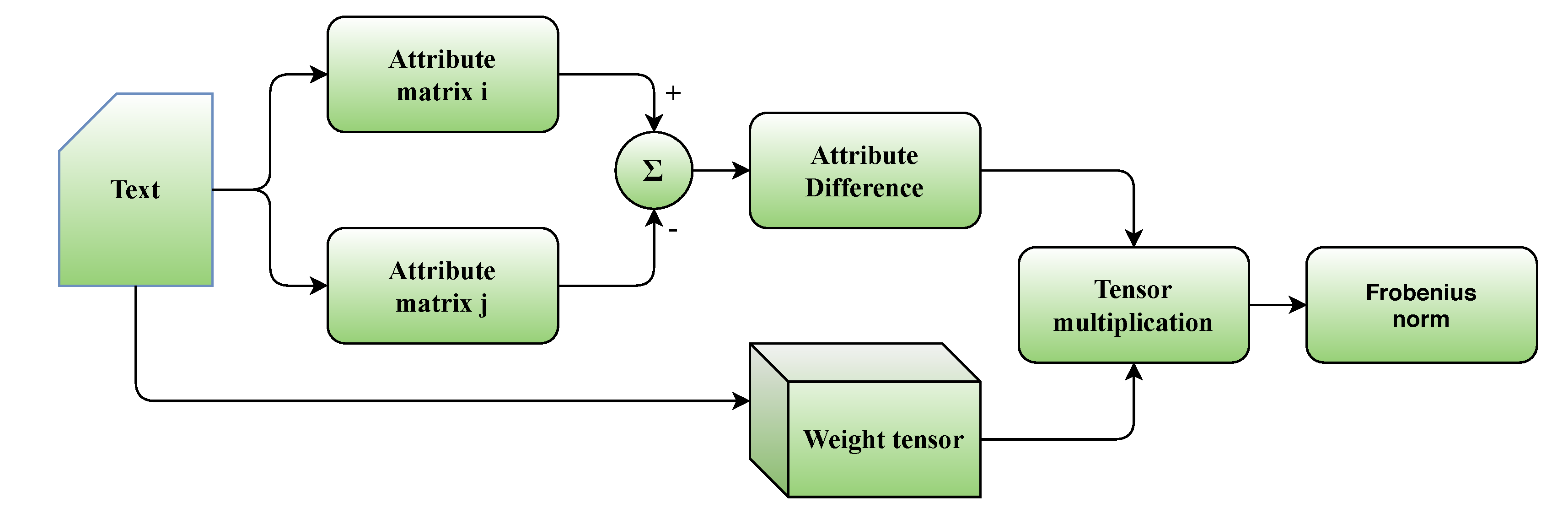
5.2. Proposed Metrics

Tensors are direct higher order generalizations of matrices and vectors. From a structural perspective a tensor is a multidimensional array indexed by an array of p integers, where p is termed the tensor order. Formally:
Definition 7
(Tensor). A p-th order tensor T , where p Z * , is a linear mapping coupling p non necessarily distinct vector spaces S k , 1 k p . If S k = R I k , then T R I 1 × × I p .
Perhaps the most important operation in tensor algebra is tensor multiplication which defines elementwise the multiplication along the k-th dimension G = X × k Y between the tensors X of order p and Y of order q, k min p , q as shown below, provided that both tensors have the same number of elements I k along the k-th dimension:
Definition 8
(Tensor multiplication). The tensor multiplication along the k-th dimension denoted by X × k Y of two tensors X R I 1 × × I k 1 × I k × I k + 1 × × I p and Y R J 1 × × J k 1 × I k × J k + 1 × J q of respective orders p and q with k min p , q is a tensor G of order p + q 2 elementwise defined as:
G i 1 , , i k 1 , i k + 1 , , i p , j 1 , , j k 1 , j k + 1 , j q = i k = 1 I k X i 1 , , i p Y j 1 , , j q .
For instance, the SVD of an arbitrary data matrix A R I 1 × I 2 can be recast as:
A = U Σ V T = Σ × 1 U × 2 V , Σ R I r × I r .
As a special case a tensor-vector product X × k v where X R I 1 × × I p and v R k I is a tensor G of order p 1 elementwise defined as:
G i 1 , , i k 1 , i k + 1 , , i p = i k = 1 I k X i 1 , , i p v i k .
The Frobenius norm of a tensor T is defined as:
T F = i 1 = 1 I 1 i p = 1 I p T i 1 , , i p 2 1 2 .
The proposed distance metric for two data points in V with the structure shown in (31) is:
g M 1 , M 2 = N × 1 M 1 M 2 × 2 M 1 M 2 × 3 M 1 M 2 F .
In Equation (36) the weight tensor N contains the correlation of each attribute as extracted from the dataset.
For the fuzzy SOM configurations the above distance is computed between each data point and each cluster center. Then the data point is considered to belong to the two closest clusters. A schematic of the proposed tensor metric is depicted at Figure 1.

5.3. Experimental Setup

The available options for the various SOM parameters are shown in Table 5.
Given the parameters of Table 5 as a starting point, a number of SOMs were implemented. Their respective configurations are shown in Table 6. In order to reduce complexity the proximity function h · , · has been chosen to be also the weight function w · . Each SOM configuration is a tuple with the following structure:
p 0 , q 0 , g · , · , h · , · , w · , η · .
In Figure 2 the architecture of the ML pipeline which has been used in this article is shown. Its linear structure as well as the relatively low number of adjustable parameters leads to a low complexity.
The SOM clustering performance will be evaluated at three distinct levels. From the most general to the most specific these are:
  • Clustering quality: As SOMs perform clustering general metrics can be used, especially since the dataset contains ground truth classes.
  • Topological map: It is possible to construct figure of merits based on the SOM operating principles. Although they are by definition SOM-specific, they nonetheless provide insight on how the self-organization of the neurons takes place while adapting to the dataset topology.
  • MBTI permuations: Finally, the dataset itself provides certain insight. Although no specific formulas can be derived, a qualitative analysis based on findings from the scientific literature.

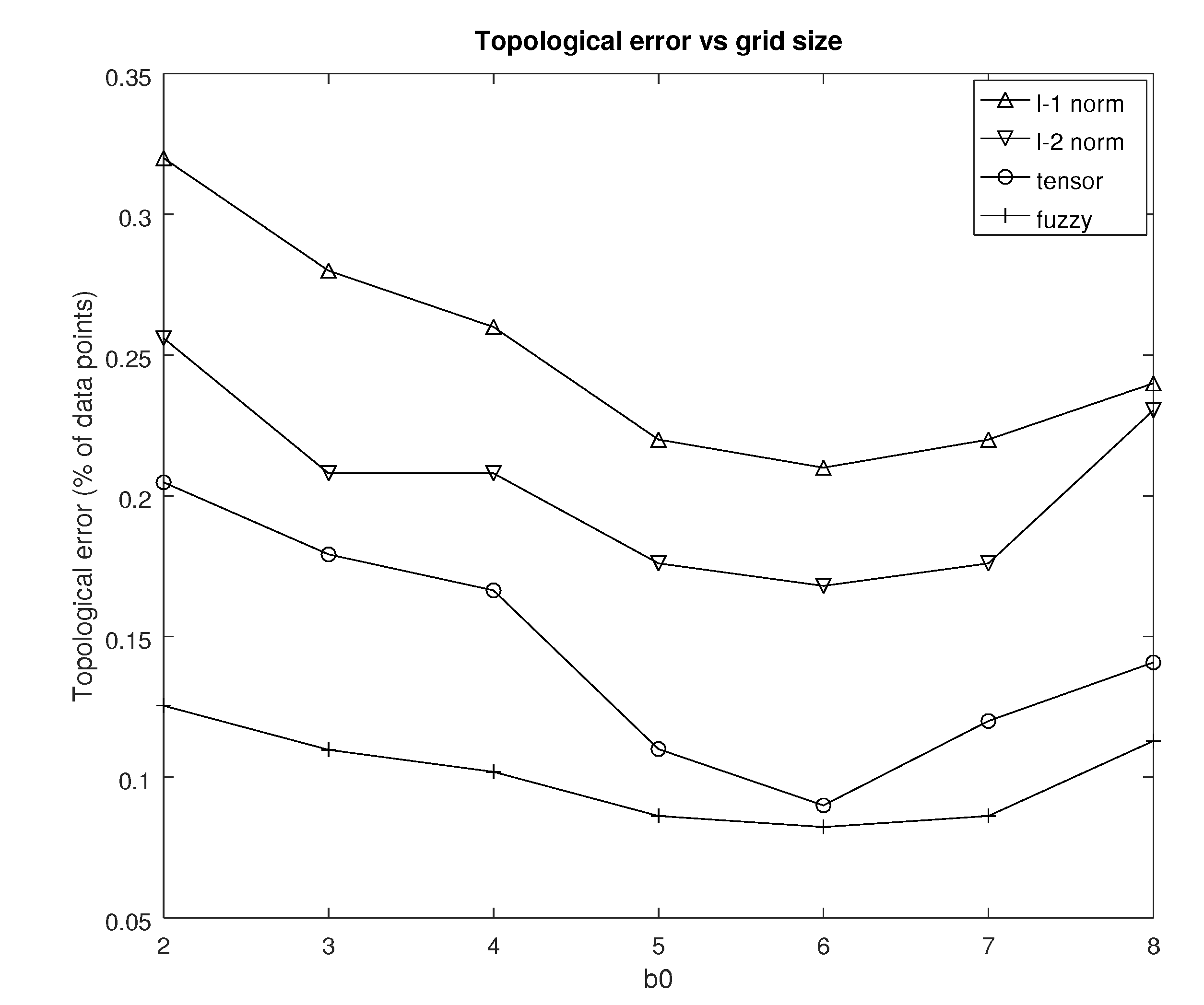
5.4. Topological Error

Because of the particular nature of the SOM, certain specialized performance metrics have been developed for it. Perhaps the most important figure of merit of this category is the topological error. The latter is defined in Equation (29). Figure 3 shows the average topological error as a percentage of the total number of data points after R 0 runs for each distance metric using the cosine rate. The reasons for the selection of this particular rate will become apparent later in this subsection. The topological error has been parameterized with respect to the SOM grid size as indexed by the parameter b 0 .
From this figure it can be inferred that the fuzzy version of the proposed tensor distance metric achieves the lowest topological error with the original tensor distance metric being a close second for most of the values of b 0 . Although 2 clearly outperforms 1 , the gap from the tensor based metrics is considerable. Representing the topologically incorrectly placed data points as a percentage of the total number of those in the dataset reveals how well the SOM can perform dimensionality reduction. With respect to the parameter b 0 there appears to be a window of b 0 5 , 6 , 7 where the topological error is minimized. Also, it appears that for this particular dataset said window is independent from the distance metric but this needs to be corroborated from further experiments.
An important metric is the distrubution of epochs before a satisfactory topological error is reached. In particular, for each distance metric the deterministic mean I 0 and variance σ 2 are of interest. Assuming for each such metric there were R 0 runs and each run required r k epochs in total, then the sample mean of the number of epochs is given by Equation (38):
I 0 = 1 R 0 k = 1 R 0 r k .
Notice that the sample mean of Equation (38) is in fact an estimator of the true stochastic mean of the number of epochs. By computing the average of R 0 samples, the estimation variance is divided by R 0 . This is typically enough to ensure convergence based on the weak law of large numbers.
Along a similar line of reasoning, the deterministic variance is similarly defined as in Equation (39). Readers familiar with estimation theory can see this is the squared natural estimator of order two.
σ 0 2 = 1 R 0 1 k = 1 R 0 r k I 0 2 .
Table 7 contains I 0 and σ 0 2 for each learning parameter rate and each distance metric. The remaining SOM parameters remained the same throughout these experiments in order to ensure fairness. Specifically b 0 was 5 and the proximity function was the Gaussian kernel.
From the entries of Table 7 the following can be deduced:
  • In each case the variance is relatively small, implying that there is a strong concentration of the number of epochs around the respective mean value. In other words, I 0 is a reliable estimator of the true number of epochs of the respective combination of distance metric and learning rate.
  • For the same learning rate the fuzzy version of the tensor distance metric consistently requires a lower number of epochs. It is followed closely by the tensor distance metric, whereas the 2 and 1 norms are way behind with the former being somewhat better than the latter.
  • Conversely, for the same metric the cosine decay rate systematically outperforms the other two options. The inverse linear decay rate may be a viable alternative, although there is a significant gap in the number of epochs. The exponential decay rates results in very slow convergence requiring almost twice the number of epochs compared to the cosine decay rate.
Notice that a lower number of epochs not only translates to quicker total response time, which is of interest when scalability becomes an issue, but also denotes that the distance metric has captured the essence of the underlying domain. This means that the SOM through the distance metric can go beyond the limitation of treating each data point merely as a collection of attributes.

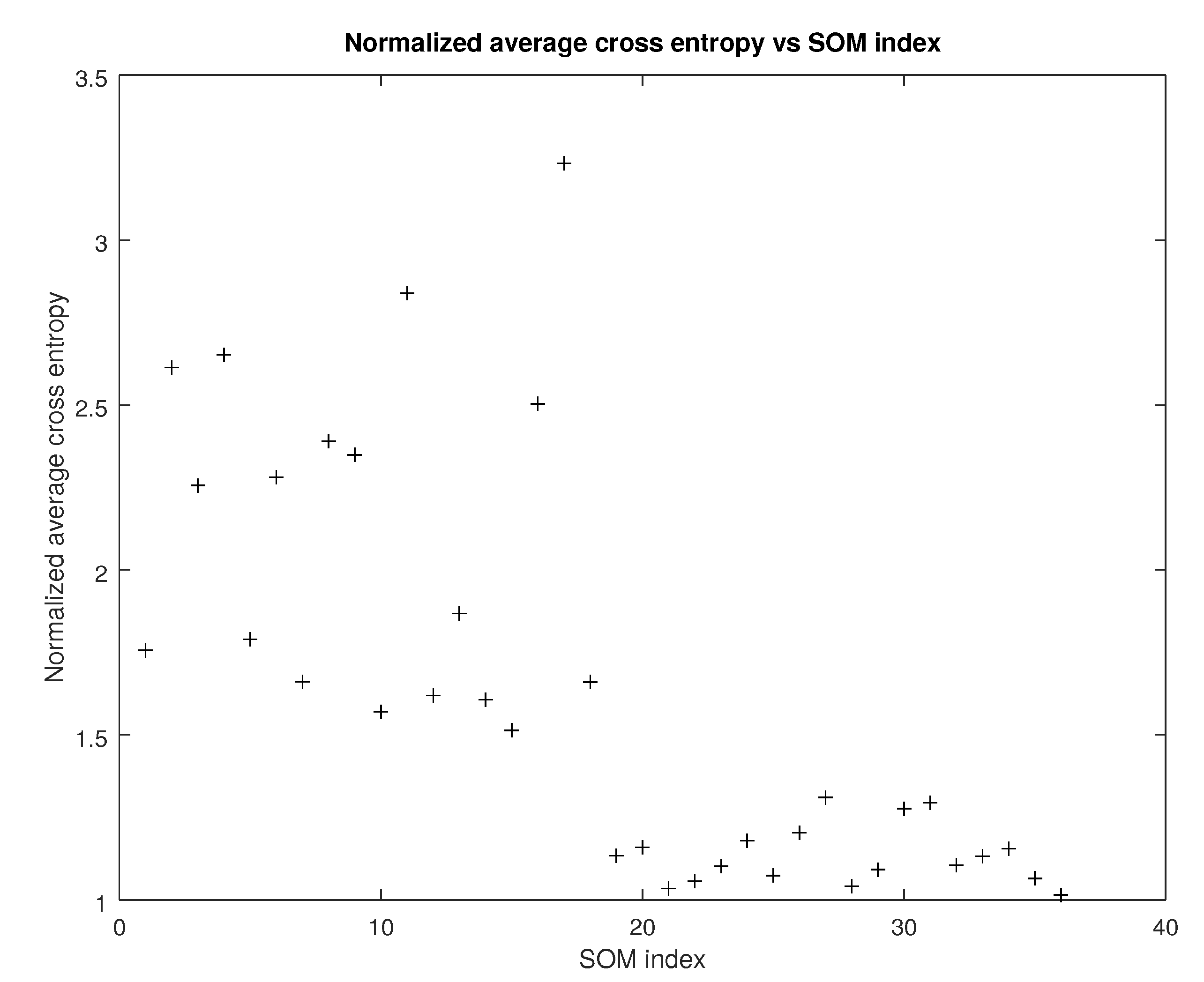
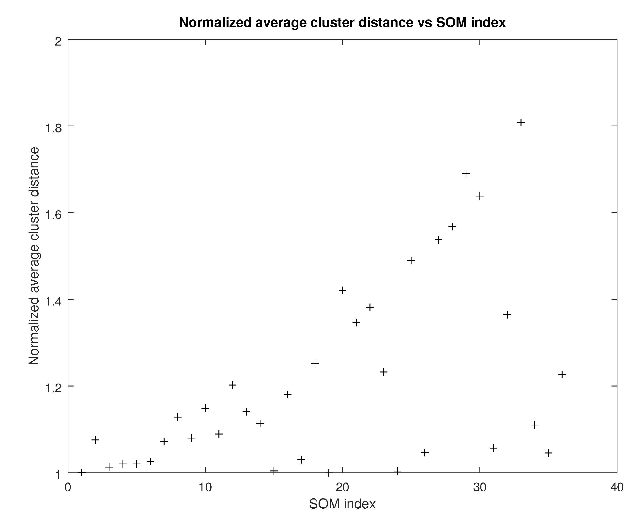
5.5. Clustering Quality

Since SOMs essentially perform clustering, it also makes sense to employ general clustering error metrics in addition to the specialized SOM ones. Since the dataset contains ground truth classes, the cross entropy metric H ¯ can be used in order to evaluate overall performance by counting the how many data points have been assigned to the wrong cluster. For the fuzzy version if one of the two clusters a data point is assigned to is the correct one, it is considered as correctly classified. In Figure 4 the normalized average cross entropy over R 0 runs is shown.
In case the ground truth classes were not available, as is the case in many clustering scenarios, the average distance d i , j between each possible distinct pair of clusters C i and C j is first computed. It is defined as the distance over all points assigned to C i from each point assigned to C j as shown in (40):
d i , j = 1 C i C j v C i y C j g x , y .
Then for the SOM configurations of Table 6 the average distance between clusters is defined as the sum of the distances over all distinct cluster pairs averaged over the number of clusters as shown in (41):
d ¯ = 2 C 0 C 0 1 i = 1 C 0 j = 2 i d i , j .
In Figure 5 the normalized d ¯ averaged over R 0 runs is shown. Observe that SOM configurations which use the proposed tensor metric yield a higher cluster distance, meaning that clusters can be better separated. This can be attributed to the fact that bounds between clusters can have more flexible shapes in comparison to the 1 and 2 norms.

5.6. MBTI Permutations
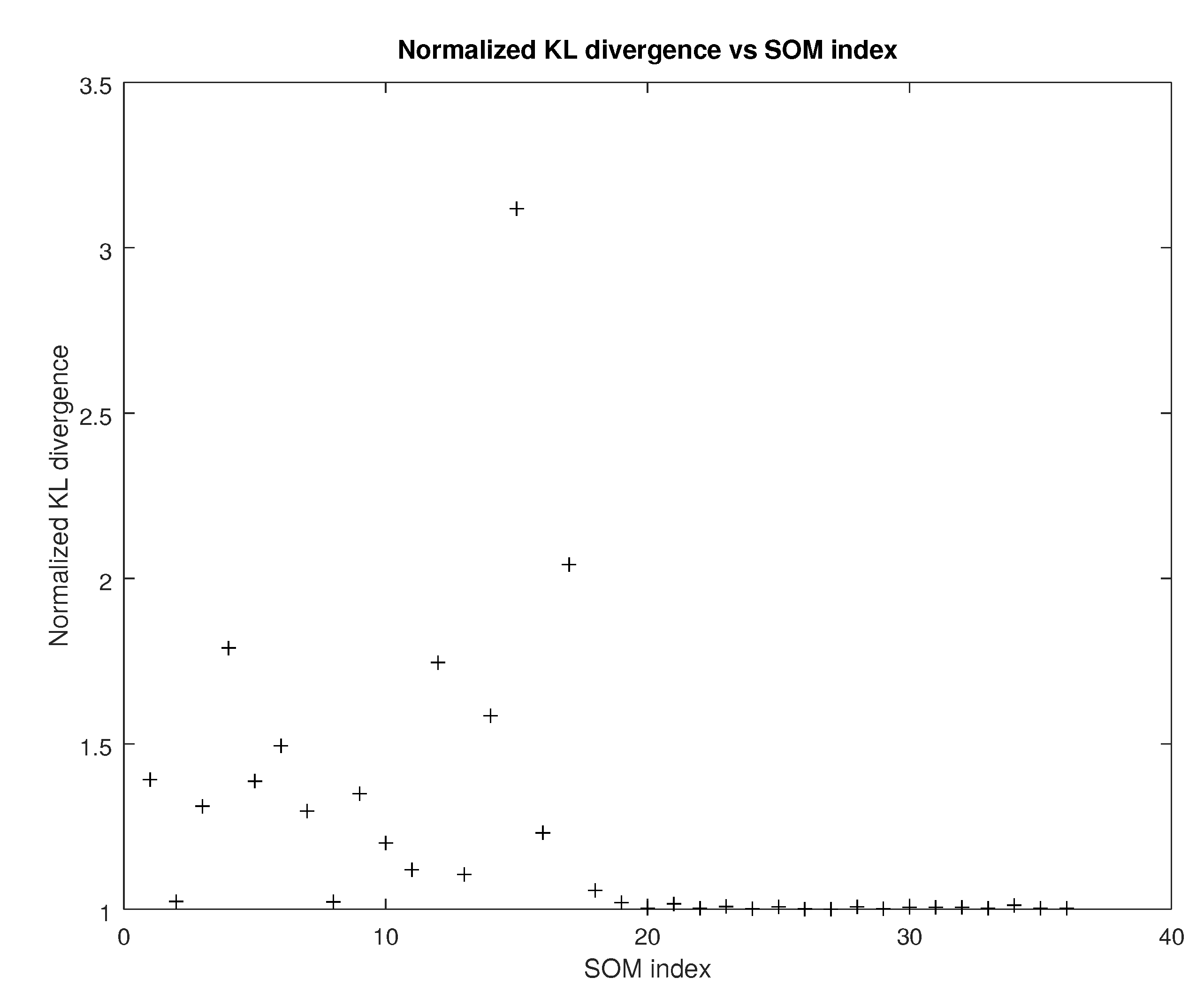
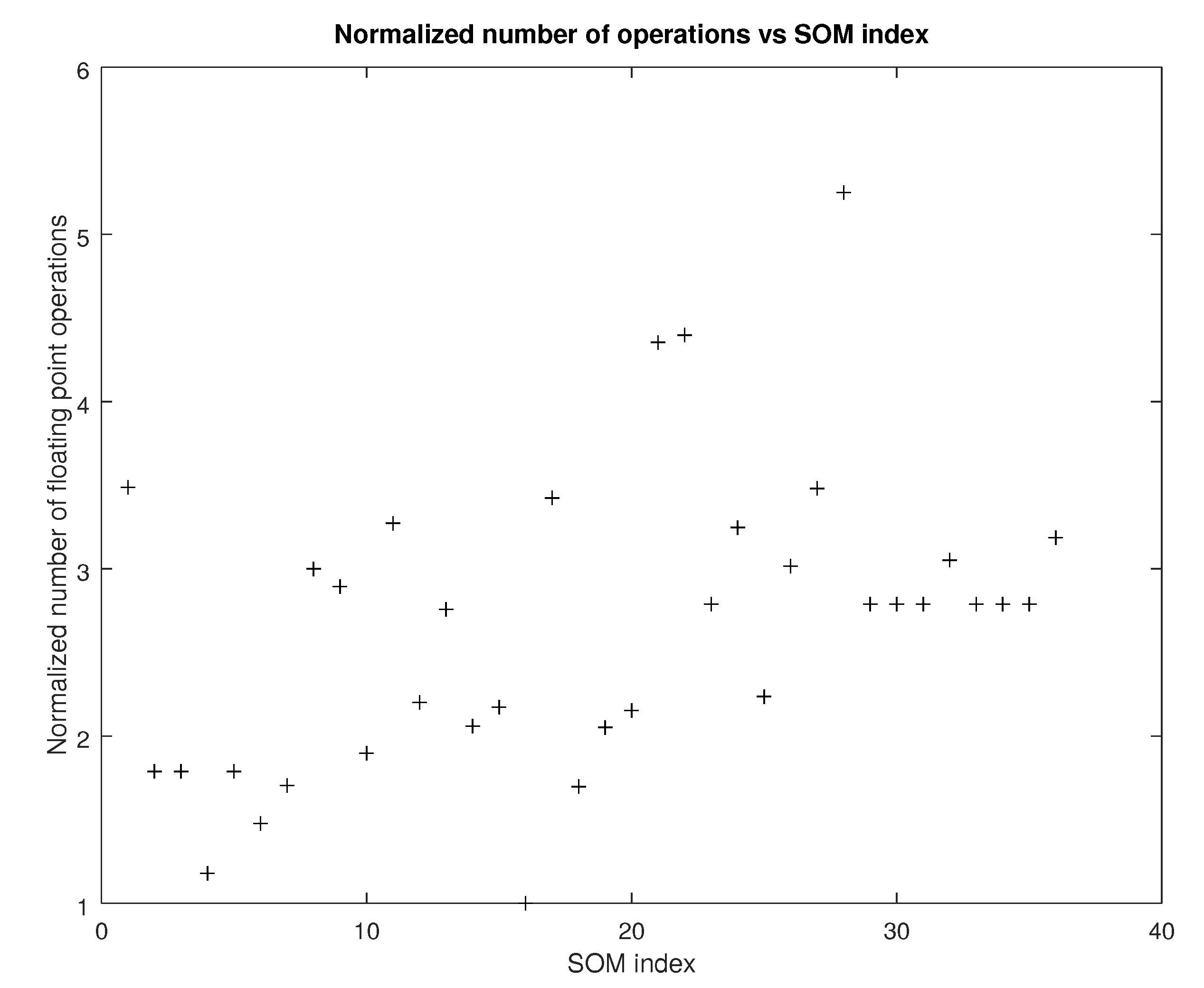
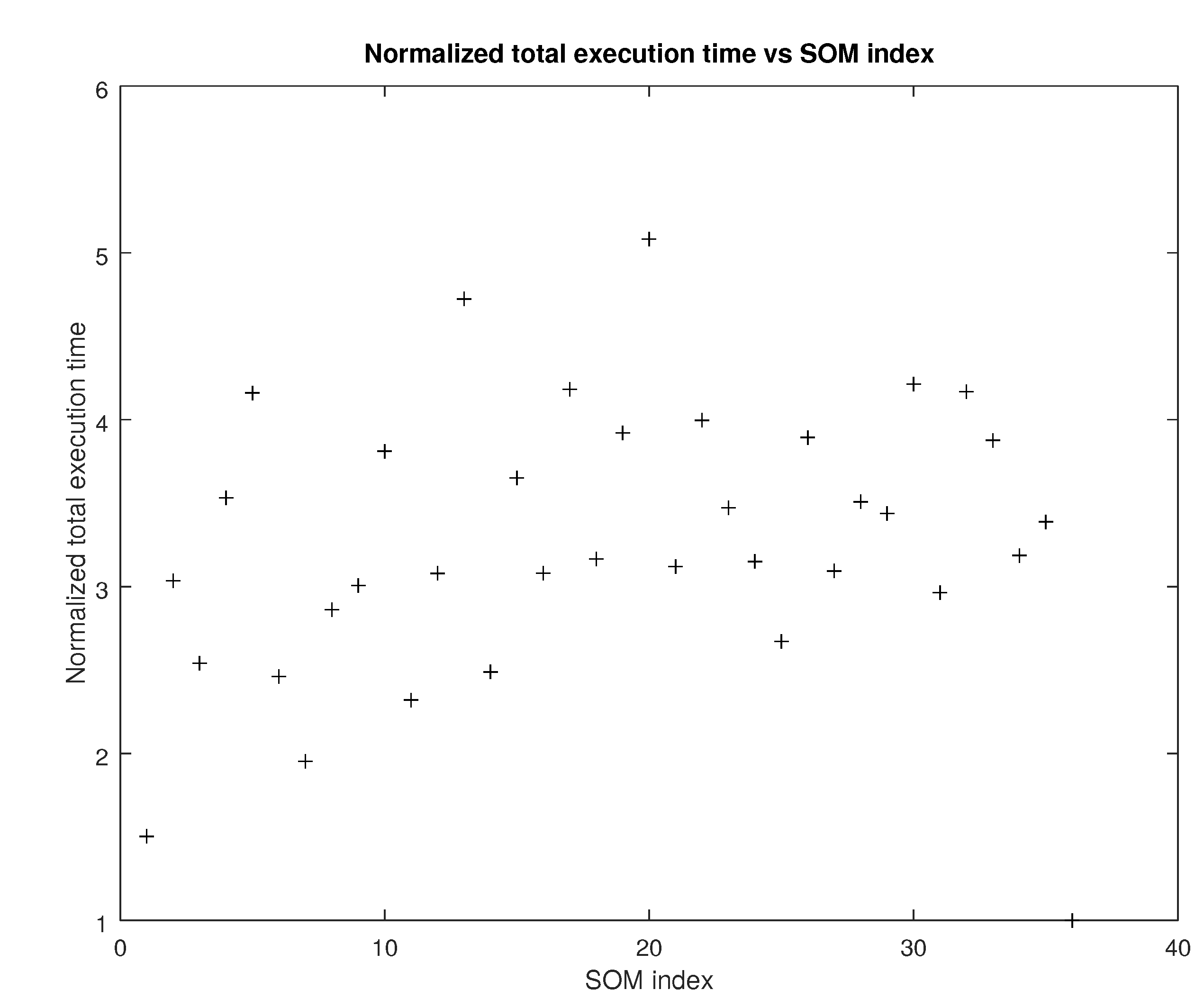
Another way of evaluating the clustering performance is by examining the natural interpretation of the resulting cognitive map based on properties of the dataset. Although this method is the least general since it is confined to the limits of a single dataset, it may lead to insights nonetheless, especially when followed by high level inspection from domain experts. The approach presented here stems from the observation that eventually each topolgical map is a permutation of Table 2. Since topology plays an important role in the continuity of the map and in the overall clustering quality, the form of the final tableau will be used. Specifically, the best map will be considered the one whose distribution of data points is the closest to that of the original dataset. To this end the Kullback-Leibler divergence will be used as shown in Equation (42):
p 1 p 2 = k p 1 k log p 1 k p 2 k = k p 1 k log p 1 k k p 1 k log p 2 k .
Notice that in Equation (42) the distributions p 1 and p 2 are not interchangeable. Instead, p 1 acts a template, whereas p 2 as a variant or an approximation thereof. In other words, the Kullback-Leibler divergence quantifies the difference of substituting p 1 with p 2 . The leftmost part of Equation (42) is the difference of the cross-entropy between p 1 and p 2 from the entropy of p 1 . Also, the index k ranges over the union of the events of both probabilities.
As stated earlier, the original Kaggle dataset was randomly sampled such that classes are balanced. Therefore, a proper topological map should have the same number of data points across all clusters. One way to measure that is to compute the Kullback-Leibler divergence of the distribution of data points assigned to clusters from the uniform distribution. Table 8 and Table 9 show the topological maps achieving the minimum and the maximum divergence.
It comes as no surprise that the topological map achieving the least divergence is in fact the original Briggs-Mayers map, namely Table 2. Notice that in this map each personality differs only by one trait from its neighboring ones. This is reminiscent of the Gray numbering scheme. Perhaps this structure leads to robustness and to higher overall clustering quality. On the contrary, the map with the largest divergence looks more like a random permutation of Table 2. Moreover, the number of traits a type differs from its neighboring ones varies.
For each SOM configuration and for each of the R 0 runs, each with a different subset of the original dataset, the resulting cognitive map the Kullback-Leibler divergence as described above was recorded. Then for each SOM configuration the average was computed and then each such average was normalized by dividing them with the minimum of them. This provides an insight on the clustering robustness of each map. In Figure 6 the normalized divergences averaged over R 0 runs are shown.
From Figure 6 it follows that the tensor-based SOM configurations have an almost uniform low Kullback-Leibler divergence from the uniform distribution. Therefore, they achieve better clustering of at least most of the R 0 available subsets.

5.7. Complexity

The complexity of the proposed method in comparison to that of the norm based methods will be examined here. Figure 7 shows the normalized number of floating point operations for each of the SOM configurations of Table 6 over R 0 iterations. Every operation count has been divided by the minimum one in order to reveal the difference the order of magnitude.
Figure 8 shows the average total execution time for each SOM configuration of Table 6 over R 0 iterations. A similar normalization with that described earlier took place here. Specifically, for each SOM configuration the total execution time averaged over all R 0 subsets of the original dataset was computed. Then, each such average was divided by the minimum one, yielding thus a measure of their relative performance.
From Figure 7 and Figure 8 it can be deduced that the added cost in floating point operations necessary for the tensor metrics is partially absorbed by the lower number of iterations. Thus, despite their increased nominal complexity, tensor based metrics remain competitive at least in terms of the total execution time.

5.8. Discussion

Based on the results presented earlier, the following can be said about the proposed methodology:
  • The cosine decay rate outperforms the inverse linear and the exponential ones. This can be explained by the adaptive nature of the cosine as well as by the fact that the exponential function decays too fast and before convergence is truly achieved.
  • Partitioning clusters in Gaussian regions results in lower error in every test case. This is explained by the less sharp shape of these regions compared to cubes or domes. Moreover, with the tensor distance metrics, which can in the general case approximate more smooth shapes, the cluster boundaries can better adapt to the topological properties of the dataset.
  • The fuzzy version of the tensor distance metric results in better performance, even a slight one, in all cases. The reason for this may be the additional flexibility since personalities sharing traits from two categories can belong to both up to an extent. On the contrary, all the other distance metrics assign a particular personality to a single cluster.
  • The complexity of the tensor metrics in terms of the number of floating point operations involved is clearly more than that of either the 1 and the 2 norm. However, because of the lower number of iterations that difference is not evident in the total execution time.
The most evident limitations of the proposed methodology, based on the preceding analysis, are the following:
  • The interpretability of the resulting cognitive map is limited by the texts of the original dataset, which in turn are answers to specific questions. Adding more cognitive dimensions to these texts would improve personality clustering quality.
  • Although the MBTI map is small, for each cognitive map there is a large number of equivalent permutations. Finding them is a critical step before any subsequent analysis takes place.
  • The curent version of the proposed methodology does not utilize neuron bias.
Several approaches have been reported in the cognitive science domain regarding the MBTI taxonomy. It should be noted that the results presented here regarding the distribution of the MBTI permutations are similar to those reported in Reference [83]. Moreover, the computational results agree with the principles for cognitive tools set forth in Reference [75].
Regarding complexity, the number of iterations required to construct the topological maps for similar map sizes are close to those reported in Reference [33]. Also the iterations obtained here are in the same order of magnitude with those of Reference [32], where fuzzy C-means is used for image partitioning, which is a comparable method the SOMs.

5.9. Recommendations

Once the algorithmic tools are available for clustering personalities based on text derived attributes according to the MBTI taxonomy, the following points should be taken into consideration:
  • Text, despite being an invaluable source of information about human traits, is not the only one. It is highly advisable that a cross check with other methods utilizing other modalities should take place.
  • In case where the personalities of two or more group members are evaluated, it is advisable that their compatibility is checked against the group tasks in order to discover potential conflict points or communication points as early as possible.

6. Conclusions and Future Work

This article focuses on a data mining pipeline for a cognitive application. At its starting stage natural language processing extracts keywords from plain text taken from the Kaggle Myers-Briggs open dataset. Each personality is represented as a wide attribute matrix. At the heart of the pipeline lies a self organizing map which is progressively trained with various combinations of learning rates, neighborhood functions, weight functions, and distance metrics to construct a cognitive map for the sixteen different personality types possible under the Myers-Briggs Type Indicator. The latter is a widespread taxonomy of human personalities based on four primary factors which is frequently used to describe team dynamics and exploit the full potential of interplay among diverse individuals. The novelty of this work comes from separating the linguistic attributes to categories depending on their semantics and using a tensor distance metric to exploit their interplay. Particular emphasis is placed on two aspects of the cognitive map. First, a multilinear distance metric is compared to the 1 and the 2 norms, both common options in similar scenarios. Second, a fuzzy version of this metric has been developed, allowing pairwise cluster overlap. The outcome of the experiments suggest that doing so leads to lower error metrics. The latter can be attributed to the added flexibility for personalities sharing traits from up to two archetypal personality types.
The work presented here can be extended in a number of ways. Regarding the algorithmic part, more specialized tensor distance metrics can be developed for various fields. For instance, in a social network analysis application the distance between two accounts can include connectivity patterns or semantic information extracted from the hashtags of the respective tweets. Moreover, clustering robustness should be investigated. The question of unbalanced classes should be addressed, either for the original dataset or in a more general context.

Author Contributions

G.D. created the theoretical framework and run the experiments, P.M. provided intuition and oversight, and A.K. and P.P. provided oversight. All authors have read and agreed to the published version of the manuscript.

Funding

This article is part of Project 451, a long term research initiative whose primary research objective is the development of novel, scalable, numerically stable, and interpretable tensor analytics.

Acknowledgments

The authors gratefully acknowledge the support of NVIDIA corporation with the donation of Titan Xp GPU used in this research.

Conflicts of Interest

The authors declare no conflict of interest.

References

  1. Kangas, J.; Kohonen, T.; Laaksonen, J. Variants of self-organizing maps. IEEE Trans. Neural Netw. 1990, 1, 93–99. [Google Scholar] [PubMed]
  2. Amato, G.; Carrara, F.; Falchi, F.; Gennaro, C.; Lagani, G. Hebbian learning meets deep convolutional neural networks. In Proceedings of the International Conference on Image Analysis and Processing; Springer: Berlin/Heidelberg, Germany, 2019; pp. 324–334. [Google Scholar]
  3. Myers, S. Myers-Briggs typology and Jungian individuation. J. Anal. Psychol. 2016, 61, 289–308. [Google Scholar] [PubMed] [Green Version]
  4. Isaksen, S.G.; Lauer, K.J.; Wilson, G.V. An examination of the relationship between personality type and cognitive style. Creat. Res. J. 2003, 15, 343–354. [Google Scholar]
  5. Poria, S.; Majumder, N.; Mihalcea, R.; Hovy, E. Emotion recognition in conversation: Research challenges, datasets, and recent advances. IEEE Access 2019, 7, 100943–100953. [Google Scholar]
  6. Batbaatar, E.; Li, M.; Ryu, K.H. Semantic-emotion neural network for emotion recognition from text. IEEE Access 2019, 7, 111866–111878. [Google Scholar]
  7. Beliy, R.; Gaziv, G.; Hoogi, A.; Strappini, F.; Golan, T.; Irani, M. From voxels to pixels and back: Self-supervision in natural-image reconstruction from fMRI. In Proceedings of the 2019 Conference on Neural Information Processing Systems NIPS, Vancouver, BC, Canada, 8–14 September 2019; pp. 6517–6527. [Google Scholar]
  8. Sidhu, G. Locally Linear Embedding and fMRI feature selection in psychiatric classification. IEEE J. Transl. Eng. Health Med. 2019, 7, 1–11. [Google Scholar]
  9. Sun, X.; Pei, Z.; Zhang, C.; Li, G.; Tao, J. Design and Analysis of a Human-Machine Interaction System for Researching Human’s Dynamic Emotion. IEEE Trans. Syst. Man Cybern. Syst. 2019. [Google Scholar] [CrossRef]
  10. Vesanto, J.; Alhoniemi, E. Clustering of the self-organizing map. IEEE Trans. Neural Netw. 2000, 11, 586–600. [Google Scholar]
  11. Kohonen, T. Exploration of very large databases by self-organizing maps. In Proceedings of the International Conference on Neural Networks (ICNN’97), Houston, TX, USA, 12 June 1997; Volume 1, pp. PL1–PL6. [Google Scholar]
  12. Kosko, B. Fuzzy cognitive maps. Int. J. Man-Mach. Stud. 1986, 24, 65–75. [Google Scholar]
  13. Taber, R. Knowledge processing with fuzzy cognitive maps. Expert Syst. Appl. 1991, 2, 83–87. [Google Scholar]
  14. Stach, W.; Kurgan, L.; Pedrycz, W.; Reformat, M. Genetic learning of fuzzy cognitive maps. Fuzzy Sets Syst. 2005, 153, 371–401. [Google Scholar]
  15. Yang, Z.; Liu, J. Learning of fuzzy cognitive maps using a niching-based multi-modal multi-agent genetic algorithm. Appl. Soft Comput. 2019, 74, 356–367. [Google Scholar]
  16. Salmeron, J.L.; Mansouri, T.; Moghadam, M.R.S.; Mardani, A. Learning fuzzy cognitive maps with modified asexual reproduction optimisation algorithm. Knowl.-Based Syst. 2019, 163, 723–735. [Google Scholar]
  17. Wu, K.; Liu, J. Robust learning of large-scale fuzzy cognitive maps via the lasso from noisy time series. Knowl.-Based Syst. 2016, 113, 23–38. [Google Scholar]
  18. Wu, K.; Liu, J. Learning large-scale fuzzy cognitive maps based on compressed sensing and application in reconstructing gene regulatory networks. IEEE Trans. Fuzzy Syst. 2017, 25, 1546–1560. [Google Scholar]
  19. Liu, Y.c.; Wu, C.; Liu, M. Research of fast SOM clustering for text information. Expert Syst. Appl. 2011, 38, 9325–9333. [Google Scholar]
  20. Drakopoulos, G.; Giannoukou, I.; Mylonas, P.; Sioutas, S. On tensor distances for self organizing maps: Clustering cognitive tasks. In Proceedings of the International Conference on Database and Expert Systems Applications Part II; Springer: Berlin/Heidelberg, Germany, 2020; Volume 12392, pp. 195–210. [Google Scholar] [CrossRef]
  21. Nam, T.M.; Phong, P.H.; Khoa, T.D.; Huong, T.T.; Nam, P.N.; Thanh, N.H.; Thang, L.X.; Tuan, P.A.; Dung, L.Q.; Loi, V.D. Self-organizing map-based approaches in DDoS flooding detection using SDN. In Proceedings of the 2018 International Conference on Information Networking (ICOIN), Chiang Mai, Thailand, 10–12 January 2018; pp. 249–254. [Google Scholar]
  22. Hawer, S.; Braun, N.; Reinhart, G. Analyzing interdependencies between factory change enablers applying fuzzy cognitive maps. Procedia CIRP 2016, 52, 151–156. [Google Scholar]
  23. Zhu, S.; Zhang, Y.; Gao, Y.; Wu, F. A Cooperative Task Assignment Method of Multi-UAV Based on Self Organizing Map. In Proceedings of the 2018 International Conference on Cyber-Enabled Distributed Computing and Knowledge Discovery (CyberC), Zhengzhou, China, 18–20 October 2018; pp. 437–4375. [Google Scholar]
  24. Ladeira, M.J.; Ferreira, F.A.; Ferreira, J.J.; Fang, W.; Falcão, P.F.; Rosa, Á.A. Exploring the determinants of digital entrepreneurship using fuzzy cognitive maps. Int. Entrep. Manag. J. 2019, 15, 1077–1101. [Google Scholar]
  25. Herrero, J.; Dopazo, J. Combining hierarchical clustering and self-organizing maps for exploratory analysis of gene expression patterns. J. Proteome Res. 2002, 1, 467–470. [Google Scholar]
  26. Imani, M.; Ghoreishi, S.F. Optimal Finite-Horizon Perturbation Policy for Inference of Gene Regulatory Networks. IEEE Intell. Syst. 2020. [Google Scholar] [CrossRef]
  27. Drakopoulos, G.; Gourgaris, P.; Kanavos, A. Graph communities in Neo4j: Four algorithms at work. Evol. Syst. 2019. [Google Scholar] [CrossRef]
  28. Gutiérrez, I.; Gómez, D.; Castro, J.; Espínola, R. A new community detection algorithm based on fuzzy measures. In Proceedings of the International Conference on Intelligent and Fuzzy Systems, Istanbul, Turkey, 23–25 July 2019; Springer: Berlin/Heidelberg, Germany, 2019; pp. 133–140. [Google Scholar]
  29. Luo, W.; Yan, Z.; Bu, C.; Zhang, D. Community detection by fuzzy relations. IEEE Trans. Emerg. Top. Comput. 2017, 8, 478–492. [Google Scholar] [CrossRef]
  30. Drakopoulos, G.; Gourgaris, P.; Kanavos, A.; Makris, C. A fuzzy graph framework for initializing k-means. IJAIT 2016, 25, 1650031:1–1650031:21. [Google Scholar] [CrossRef]
  31. Yang, C.H.; Chuang, L.Y.; Lin, Y.D. Epistasis Analysis using an Improved Fuzzy C-means-based Entropy Approach. IEEE Trans. Fuzzy Syst. 2019, 28, 718–730. [Google Scholar] [CrossRef]
  32. Tang, Y.; Ren, F.; Pedrycz, W. Fuzzy C-means clustering through SSIM and patch for image segmentation. Appl. Soft Comput. 2020, 87, 105928. [Google Scholar] [CrossRef]
  33. Felix, G.; Nápoles, G.; Falcon, R.; Froelich, W.; Vanhoof, K.; Bello, R. A review on methods and software for fuzzy cognitive maps. Artif. Intell. Rev. 2019, 52, 1707–1737. [Google Scholar] [CrossRef]
  34. Etingof, P.; Gelaki, S.; Nikshych, D.; Ostrik, V. Tensor Categories; American Mathematical Soc.: Providence, RI, USA, 2016; Volume 205. [Google Scholar]
  35. Batselier, K.; Chen, Z.; Liu, H.; Wong, N. A tensor-based volterra series black-box nonlinear system identification and simulation framework. In Proceedings of the 2016 IEEE/ACM International Conference on Computer-Aided Design (ICCAD), Austin, TX, USA, 7–10 November 2016; pp. 1–7. [Google Scholar]
  36. Batselier, K.; Chen, Z.; Wong, N. Tensor Network alternating linear scheme for MIMO Volterra system identification. Automatica 2017, 84, 26–35. [Google Scholar] [CrossRef] [Green Version]
  37. Batselier, K.; Ko, C.Y.; Wong, N. Tensor network subspace identification of polynomial state space models. Automatica 2018, 95, 187–196. [Google Scholar] [CrossRef] [Green Version]
  38. Battaglino, C.; Ballard, G.; Kolda, T.G. A practical randomized CP tensor decomposition. SIAM J. Matrix Anal. Appl. 2018, 39, 876–901. [Google Scholar] [CrossRef]
  39. Sidiropoulos, N.D.; De Lathauwer, L.; Fu, X.; Huang, K.; Papalexakis, E.E.; Faloutsos, C. Tensor decomposition for signal processing and machine learning. IEEE Trans. Signal Process. 2017, 65, 3551–3582. [Google Scholar] [CrossRef]
  40. Ragusa, E.; Gastaldo, P.; Zunino, R.; Cambria, E. Learning with similarity functions: A tensor-based framework. Cogn. Comput. 2019, 11, 31–49. [Google Scholar] [CrossRef]
  41. Lu, W.; Chung, F.L.; Jiang, W.; Ester, M.; Liu, W. A deep Bayesian tensor-based system for video recommendation. ACM Trans. Inf. Syst. 2018, 37, 1–22. [Google Scholar] [CrossRef]
  42. Drakopoulos, G.; Stathopoulou, F.; Kanavos, A.; Paraskevas, M.; Tzimas, G.; Mylonas, P.; Iliadis, L. A genetic algorithm for spatiosocial tensor clustering: Exploiting TensorFlow potential. Evol. Syst. 2020, 11, 491–501. [Google Scholar] [CrossRef]
  43. Bao, Y.T.; Chien, J.T. Tensor classification network. In Proceedings of the 2015 IEEE 25th International Workshop on Machine Learning for Signal Processing (MLSP), Boston, MA, USA, 17–20 September 2015; pp. 1–6. [Google Scholar]
  44. Yu, D.; Deng, L.; Seide, F. The deep tensor neural network with applications to large vocabulary speech recognition. IEEE Trans. Audio Speech Lang. Process. 2012, 21, 388–396. [Google Scholar] [CrossRef]
  45. Drakopoulos, G.; Mylonas, P. Evaluating graph resilience with tensor stack networks: A Keras implementation. Neural Comput. Appl. 2020, 32, 4161–4176. [Google Scholar] [CrossRef]
  46. Hore, V.; Viñuela, A.; Buil, A.; Knight, J.; McCarthy, M.I.; Small, K.; Marchini, J. Tensor decomposition for multiple-tissue gene expression experiments. Nat. Genet. 2016, 48, 1094. [Google Scholar] [CrossRef] [PubMed] [Green Version]
  47. Zhang, C.; Fu, H.; Liu, S.; Liu, G.; Cao, X. Low-rank tensor constrained multiview subspace clustering. In Proceedings of the IEEE international conference on computer vision, Santiago, Chile, 7–13 December 2015; pp. 1582–1590. [Google Scholar]
  48. Cao, X.; Wei, X.; Han, Y.; Lin, D. Robust face clustering via tensor decomposition. IEEE Trans. Cybern. 2014, 45, 2546–2557. [Google Scholar] [CrossRef]
  49. Zaharia, M.; Xin, R.S.; Wendell, P.; Das, T.; Armbrust, M.; Dave, A.; Meng, X.; Rosen, J.; Venkataraman, S.; Franklin, M.J.; et al. Apache Spark: A unified engine for big data processing. Commun. ACM 2016, 59, 56–65. [Google Scholar] [CrossRef]
  50. Alexopoulos, A.; Drakopoulos, G.; Kanavos, A.; Mylonas, P.; Vonitsanos, G. Two-step classification with SVD preprocessing of distributed massive datasets in Apache Spark. Algorithms 2020, 13, 71. [Google Scholar] [CrossRef] [Green Version]
  51. Yang, H.K.; Yong, H.S. S-PARAFAC: Distributed tensor decomposition using Apache Spark. J. KIISE 2018, 45, 280–287. [Google Scholar] [CrossRef]
  52. Bezanson, J.; Edelman, A.; Karpinski, S.; Shah, V.B. Julia: A fresh approach to numerical computing. SIAM Rev. 2017, 59, 65–98. [Google Scholar] [CrossRef] [Green Version]
  53. Bezanson, J.; Chen, J.; Chung, B.; Karpinski, S.; Shah, V.B.; Vitek, J.; Zoubritzky, L. Julia: Dynamism and performance reconciled by design. Proc. ACM Program. Lang. 2018, 2, 1–23. [Google Scholar] [CrossRef] [Green Version]
  54. Lee, J.; Kim, Y.; Song, Y.; Hur, C.K.; Das, S.; Majnemer, D.; Regehr, J.; Lopes, N.P. Taming undefined behavior in LLVM. ACM SIGPLAN Not. 2017, 52, 633–647. [Google Scholar] [CrossRef]
  55. Innes, M. Flux: Elegant machine learning with Julia. J. Open Source Softw. 2018, 3, 602. [Google Scholar] [CrossRef] [Green Version]
  56. Besard, T.; Foket, C.; De Sutter, B. Effective extensible programming: Unleashing Julia on GPUs. IEEE Trans. Parallel Distrib. Syst. 2018, 30, 827–841. [Google Scholar] [CrossRef] [Green Version]
  57. Mogensen, P.K.; Riseth, A.N. Optim: A mathematical optimization package for Julia. J. Open Source Softw. 2018, 3. [Google Scholar] [CrossRef]
  58. Ruthotto, L.; Treister, E.; Haber, E. jinv–A flexible Julia package for PDE parameter estimation. SIAM J. Sci. Comput. 2017, 39, S702–S722. [Google Scholar] [CrossRef] [Green Version]
  59. Krämer, S.; Plankensteiner, D.; Ostermann, L.; Ritsch, H. QuantumOptics.jl: A Julia framework for simulating open quantum systems. Comput. Phys. Commun. 2018, 227, 109–116. [Google Scholar] [CrossRef] [Green Version]
  60. Witte, P.A.; Louboutin, M.; Kukreja, N.; Luporini, F.; Lange, M.; Gorman, G.J.; Herrmann, F.J. A large-scale framework for symbolic implementations of seismic inversion algorithms in Julia. Geophysics 2019, 84, F57–F71. [Google Scholar] [CrossRef]
  61. Pittenger, D.J. The utility of the Myers-Briggs type indicator. Rev. Educ. Res. 1993, 63, 467–488. [Google Scholar] [CrossRef]
  62. Gordon, A.M.; Jackson, D. A Balanced Approach to ADHD and Personality Assessment: A Jungian Model. N. Am. J. Psychol. 2019, 21, 619–646. [Google Scholar]
  63. Lake, C.J.; Carlson, J.; Rose, A.; Chlevin-Thiele, C. Trust in name brand assessments: The case of the Myers-Briggs type indicator. Psychol.-Manag. J. 2019, 22, 91. [Google Scholar] [CrossRef]
  64. Stein, R.; Swan, A.B. Evaluating the validity of Myers-Briggs Type Indicator theory: A teaching tool and window into intuitive psychology. Soc. Personal. Psychol. Compass 2019, 13, e12434. [Google Scholar] [CrossRef]
  65. Plutchik, R.E.; Conte, H.R. Circumplex Models of Personality and Emotions; American Psychological Association: Washington, DC, USA, 1997. [Google Scholar]
  66. Ekman, P. Darwin, deception, and facial expression. Ann. N. Y. Acad. Sci. 2003, 1000, 205–221. [Google Scholar] [CrossRef] [PubMed] [Green Version]
  67. Furnham, A. Myers-Briggs type indicator (MBTI). In Encyclopedia of Personality and Individual Differences; Springer: Berlin/Heidelberg, Germany, 2020; pp. 3059–3062. [Google Scholar]
  68. Xie, Y.; Liang, R.; Liang, Z.; Huang, C.; Zou, C.; Schuller, B. Speech emotion classification using attention-based LSTM. IEEE/ACM Trans. Audio Speech Lang. Process. 2019, 27, 1675–1685. [Google Scholar] [CrossRef]
  69. Kim, Y.; Moon, J.; Sung, N.J.; Hong, M. Correlation between selected gait variables and emotion using virtual reality. J. Ambient. Intell. Humaniz. Comput. 2019, 1–8. [Google Scholar] [CrossRef]
  70. Zheng, W.; Yu, A.; Fang, P.; Peng, K. Exploring collective emotion transmission in face-to-face interactions. PLoS ONE 2020, 15, e0236953. [Google Scholar] [CrossRef]
  71. Nguyen, T.L.; Kavuri, S.; Lee, M. A multimodal convolutional neuro-fuzzy network for emotion understanding of movie clips. Neural Netw. 2019, 118, 208–219. [Google Scholar] [CrossRef]
  72. Mishro, P.K.; Agrawal, S.; Panda, R.; Abraham, A. A novel type-2 fuzzy C-means clustering for brain MR image segmentation. IEEE Trans. Cybern. 2020. [Google Scholar] [CrossRef]
  73. Sheldon, S.; El-Asmar, N. The cognitive tools that support mentally constructing event and scene representations. Memory 2018, 26, 858–868. [Google Scholar] [CrossRef]
  74. Zap, N.; Code, J. Virtual and augmented reality as cognitive tools for learning. In EdMedia+ Innovate Learning; Association for the Advancement of Computing in Education (AACE): Waynesville, NC, USA, 2016; pp. 1340–1347. [Google Scholar]
  75. Spevack, S.C. Cognitive Tools and Cognitive Styles: Windows into the Culture-Cognition System. Ph.D. Thesis, UC Merced, Merced, CA, USA, 2019. [Google Scholar]
  76. Lajoie, S.P. Computers As Cognitive Tools: Volume II, No More Walls; Routledge: London, UK, 2020. [Google Scholar]
  77. Abiri, R.; Borhani, S.; Sellers, E.W.; Jiang, Y.; Zhao, X. A comprehensive review of EEG-based brain–computer interface paradigms. J. Neural Eng. 2019, 16, 011001. [Google Scholar] [CrossRef]
  78. Ramadan, R.A.; Vasilakos, A.V. Brain computer interface: Control signals review. Neurocomputing 2017, 223, 26–44. [Google Scholar] [CrossRef]
  79. Sakhavi, S.; Guan, C.; Yan, S. Learning temporal information for brain-computer interface using convolutional neural networks. IEEE Trans. Neural Netw. Learn. Syst. 2018, 29, 5619–5629. [Google Scholar] [CrossRef] [PubMed]
  80. Kaur, B.; Singh, D.; Roy, P.P. Age and gender classification using brain–computer interface. Neural Comput. Appl. 2019, 31, 5887–5900. [Google Scholar] [CrossRef]
  81. Beale, M.H.; Hagan, M.T.; Demuth, H.B. Neural Network Toolbox User’s Guide; The Mathworks Inc.: Natick, MA, USA, 2010. [Google Scholar]
  82. Graillat, S.; Ibrahimy, Y.; Jeangoudoux, C.; Lauter, C. A Parallel Compensated Horner Scheme. In Proceedings of the SIAM Conference on Computational Science and Engineering (CSE), Atlanta, GA, USA, 3 March–27 February 2017. [Google Scholar]
  83. Amirhosseini, M.H.; Kazemian, H. Machine Learning Approach to Personality Type Prediction Based on the Myers–Briggs Type Indicator®. Multimodal Technol. Interact. 2020, 4, 9. [Google Scholar] [CrossRef] [Green Version]
Figure 1. Schematic of the proposed metric (source: authors).
Mathematics 08 01898 g001
Figure 2. Architecture of the proposed pipeline (source: authors).
Mathematics 08 01898 g002
Figure 3. Topological error vs b 0 (source: authors).
Mathematics 08 01898 g003
Figure 4. Normalized cross entropy vs SOM index (source: authors).
Mathematics 08 01898 g004
Figure 5. Normalized average cluster distance vs SOM index (source: authors).
Mathematics 08 01898 g005
Figure 6. Normalized divergence vs SOM index (source: authors).
Mathematics 08 01898 g006
Figure 7. Normalized number of floating point operations vs SOM index (source: authors).
Mathematics 08 01898 g007
Figure 8. Normalized total execution time vs SOM index (source: authors).
Mathematics 08 01898 g008
Table 1. Notation of this article.
SymbolMeaning
= Definition or equality by definition
s 1 , , s n or s k k = 1 n Set with elements s 1 , , s n
S or s 1 , , s n Set cardinality
× k Tensor multiplication along the k-th direction
vec · Vectorize operation for matrices and tensors
loc · Location function for data points
invloc · Inverse location relationship for neurons
weight u Synaptic weights of neuron u
bias u Bias of neuron u
Γ u Neighborhood of neuron u
Δ u Cover of neuron u
p 1 p 2 Kullback-Leibler divergence between discrete distributions p 1 and p 2
Table 2. Myers-Briggs Type Indicator (MBTI) taxonomy (source: [61]).
TypeAttributesTypeAttributes
ISTJIntroversion, Sensing, Thinking, JudgingINFJIntroversion, Intuition, Feeling, Judging
ISTPIntroversion, Sensing, Thinking, PerceivingINFPIntroversion, Intuition, Feeling, Perceiving
ESTPExtraversion, Sensing, Thinking, PerceivingENFPExtraversion, Intuition, Feeling, Perceiving
ESTJExtraversion, Sensing, Thinking, JudgingENFJExtraversion, Intuition, Feeling, Judging
ISFJIntroversion, Sensing, Feeling, JudgingINTJIntroversion, Intuition, Thinking, Judging
ISFPIntroversion, Sensing, Feeling, PerceivingINTPIntroversion, Intuition, Thinking, Perceiving
ESFPExtraversion, Sensing, Feeling, PerceivingENTPExtraversion, Intuition, Thinking, Perceiving
ESFJExtraversion, Sensing, Feeling, JudgingENTJExtraversion, Intuition, Thinking, Judging
Table 3. Cluster shapes (source: authors).
NeighborhoodWeightShapeNeighborhoodWeightShape
SquareSquareCubeTriangularTriangularPyramid
SquareTriangularPyramidCircularSemicircularDome
SquareSemicircularDomeGaussianGaussian3D Gaussian
Table 4. Extracted attributes.
AttributePosition in (31)
Normalized number of words m 1 , 1
Normalized number of characters m 1 , 2
Normalized number of punctuation marks m 1 , 3
Normalized number of question marks m 1 , 4
Normalized number of exclamation points m 1 , 5
Normalized number of occurences of two or more ’.’ m 1 , 6
Normalized number of positive words m 2 , 1
Normalized number of negative words m 2 , 2
Normalized number of self-references m 2 , 3
Normalized number of references to others m 2 , 4
Normalized number of words pertaining to emotion m 2 , 5
Normalized number of words pertaining to reason m 2 , 6
Table 5. Options for the self organizing map (SOM) parameters (source: authors).
ParameterOptions
Synaptic weight initializationRandom
Bias mechanismNot implemented
Neighborhood Γ u shapeCross
Distance function g · , · Tensor (T), Fuzzy tensor (F), 1 norm (L1), 2 norm (L2)
Proximity function h · , · Gaussian (G), Circular (C), Rectangular (R)
Cover threshold η 0 - Equation (27) 0.5
Weight function in C Gaussian, Circular, Rectangular (as above)
Gaussian μ 0 = 0 , σ 0 2 = 8
Circular ρ 0 = 4
Rectangular a 0 = 4
Learning rate parameterCosine (S), Inverse linear (L), Inverse quadratic (Q), Exponential (E)
Cosine r 0 = 40
Inverse linear γ 2 = 1 , γ 1 = 0.025 , γ 0 = 1
Exponential γ 0 = 1 , γ 1 = 0.125
Grid size b 0 and b 1 - Equation (30) b 0 2 , , 8 , b 1 = 0
Number of classes C 0 16
Number of rows per class N 0 256
Number of attributes2 Q 0
Number of runs R 0 100
Table 6. Indices of SOM configurations (source: authors).
#Configuration#Configuration#Configuration#Configuration
1 p 0 , p 0 , L 1 , C , C , S 10 p 0 , p 0 , L 2 , C , C , S 19 p 0 , p 0 , T , C , C , S 28 p 0 , p 0 , F , C , C , S
2 p 0 , p 0 , L 1 , R , R , S 11 p 0 , p 0 , L 2 , R , R , S 20 p 0 , p 0 , T , R , R , S 29 p 0 , p 0 , F , R , R , S
3 p 0 , p 0 , L 1 , G , G , S 12 p 0 , p 0 , L 2 , G , G , S 21 p 0 , p 0 , T , G , G , S 30 p 0 , p 0 , F , G , G , S
4 p 0 , p 0 , L 1 , C , C , L 13 p 0 , p 0 , L 2 , C , C , L 22 p 0 , p 0 , T , C , C , L 31 p 0 , p 0 , F , C , C , L
5 p 0 , p 0 , L 1 , R , R , L 14 p 0 , p 0 , L 2 , R , R , L 23 p 0 , p 0 , T , R , R , L 32 p 0 , p 0 , F , R , R , L
6 p 0 , p 0 , L 1 , G , G , L 15 p 0 , p 0 , L 2 , G , G , L 24 p 0 , p 0 , T , G , G , L 33 p 0 , p 0 , F , G , G , L
7 p 0 , p 0 , L 1 , C , C , E 16 p 0 , p 0 , L 2 , C , C , E 25 p 0 , p 0 , T , C , C , E 34 p 0 , p 0 , F , C , C , E
8 p 0 , p 0 , L 1 , R , R , E 17 p 0 , p 0 , L 2 , R , R , E 26 p 0 , p 0 , T , R , R , E 35 p 0 , p 0 , F , R , R , E
9 p 0 , p 0 , L 1 , G , G , E 18 p 0 , p 0 , L 2 , G , G , E 27 p 0 , p 0 , T , G , G , E 36 p 0 , p 0 , F , G , G , E
Table 7. Mean and variance of the number of epochs (source: authors).
CosineInv. linearExponential
1 norm I 0 = 26.4417 / σ 0 2 = 12.3873 I 0 = 27.500 / σ 0 2 = 16.8865 I 0 = 33.1125 / σ 0 2 = 14.8873
2 norm I 0 = 22.3334 / σ 0 2 = 13.0228 I 0 = 24.667 / σ 0 2 = 14.3098 I 0 = 31.8333 / σ 0 2 = 15.5642
Tensor I 0 = 18.8731 / σ 0 2 = 11.6686 I 0 = 20.2504 / σ 0 2 = 12.7633 I 0 = 26.0021 / σ 0 2 = 14.6574
Fuzzy I 0 = 14.4457 / σ 0 2 = 12.1282 I 0 = 18.3333 / σ 0 2 = 12.6645 I 0 = 25.3333 / σ 0 2 = 14.0995
Table 8. Clustering attaining the minimum divergence (source: authors).
ISTJISFJINFJINTJ
ISTPISFPINFPINTP
ESTPESFPENFPENTP
ESTJESFJENFJENTJ
Table 9. Clustering attaining the maximum divergence (source: authors).
ENFJISFPENFJESFP
ISTJINTPESTJISFJ
INTJINFJENTPISTP
ESFJENTJESTPISFP
Publisher’s Note: MDPI stays neutral with regard to jurisdictional claims in published maps and institutional affiliations.

