Soliton Solutions for a Nonisospectral Semi-Discrete Ablowitz–Kaup–Newell–Segur Equation

Abstract

In this paper, we study a nonisospectral semi-discrete Ablowitz–Kaup–Newell–Segur equation. Multisoliton solutions for this equation are given by Hirota’s method. Dynamics of some soliton solutions are analyzed and illustrated by asymptotic analysis. Multisoliton solutions and dynamics to a nonisospectral semi-discrete modified Korteweg-de Vries equation are also discussed.

1. Introduction

Nonisospectral integrable system [1,2,3] has attracted a great deal of interest and has been studied for many years from various view points, such as integrability and exact solutions. Compared with the isospectral integrable system, a nonisospectral integrable system is usually related to time-dependent spectral parameters and has time-varying solitary wave solutions. In general, depending on the linear problems, a nonisospectral integrable hierarchy can be derived from the Lax equation, zero curvature equation, or in the frame of Kac–Moody algebra, etc. [4,5,6]. The nonisospectral flows play the role of master symmetries and can be applied to generate time-dependent symmetries [7,8]. With regard to solutions for the nonisospectral integrable system, various of approaches have been developed, such as Inverse Scattering Transform, Bäcklund transformation, Darboux transformation, Hirota’s method, and the Wronskian technique [9,10,11,12,13].

In recent decades, the semi-discrete integrable system, i.e., the system given by an integrable partial differential-difference equation, has become an increasingly popular topic. Some prototypical examples include Toda lattice, Volterra lattice, semi-discrete nonlinear Schrödinger equation, semi-discrete modified Korteweg–de Vries (mKdV) equation, and so on. Such type of equations relate to many branches of mathematical theories and and play a central role in many fields. For instance, the semi-discrete nonlinear Schrödinger equation (also known as the self-trapping equation) has a number of applications in molecular physics, nonlinear optics, and in other fields [14,15]. The semi-discrete mKdV equation arises in a wide variety of fields, such as plasma physics, electromagnetic waves in ferromagnetic, antiferromagnetic, or dielectric systems.

Generally speaking, a continuous equation could have several discrete versions upon the discretisation procedure. Until now, many results for semi-discrete Ablowitz–Kaup–Newell–Segur (AKNS) type equations have been derived [16,17,18,19,20,21]. In [22] (see also [23]), Ablowitz and Ladik propose a semi-discrete spectral problem, called the Ablowitz–Ladik spectral problem,

$$\begin{array}{c}\hfill \left(\begin{array}{c}{\varphi }_{1,n+1}\\ {\varphi }_{2,n+1}\end{array}\right)={\mathit{M}}_n\left(\begin{array}{c}{\varphi }_{1,n}\\ {\varphi }_{2,n}\end{array}\right),{\mathit{M}}_n=\left(\begin{array}{cc}\lambda & u_n\\ v_n& \frac{1}{\lambda }\end{array}\right)\end{array}$$

(1)

with spectral parameter $\lambda$ and potentials $u_n=u(n,t)$ and $v_n=v(n,t)$. The spectral problem (1) can be viewed as a semi-discrete counterpart of the famous AKNS spectral problem [24]. By imposing time evolution,

$$\begin{array}{c}\hfill {\left(\begin{array}{c}{\varphi }_{1,n}\\ {\varphi }_{2,n}\end{array}\right)}_t={\mathit{N}}_n\left(\begin{array}{c}{\varphi }_{1,n}\\ {\varphi }_{2,n}\end{array}\right),{\mathit{M}}_n=\left(\begin{array}{cc}{A}_n& B_n\\ C_n& D_n\end{array}\right),\end{array}$$

(2)

then, by zero curve equation ${\mathit{M}}_{n,t}={\mathit{N}}_{n+1}{\mathit{M}}_n-{\mathit{M}}_n{\mathit{N}}_n$, the Ablowitz–Ladik lattice hierarchy can be derived. When ${\lambda }_t\ne 0$, the corresponding hierarchy is called nonisospectral Ablowitz–Ladik lattice hierarchy [25]. The spectral problem (1), coupled with different time evolution parts, has provided Lax integrabilities for many nonisospectral semi-discrete integrable systems, such as a nonisospectral semi-discrete nonlinear Schrödinger equation, nonisospectral semi-discrete mKdV equation, and so forth. Recently, starting from nonisospectral flows of the Ablowitz–Ladik lattice hierarchy, by suitable linear combinations, Zhang et al. get nonisospectral AKNS flows, which go to the continuous nonisospectral AKNS flows under a continuous limit [26].

Up to now, several works have been done to search for exact solutions for nonisospectral semi-discrete integrable systems. In [27,28], Inverse Scattering Transform was used to construct multisoliton solutions of the nonisospectral Ablowitz–Ladik hierarchy. Recently, N-soliton solutions to a nonisospectral Ablowitz–Ladik type equation have been investigated by using the Hirota’s method and Casorati technique [29]. In addition, based on Hankel type determinants, Chen et al. present solutions for a nonisospectral Toda lattice [30] as well as the first and second members in the nonisospectral extended Volterra lattice hierarchy [31].

In this paper, we are interested in the multisoliton solutions for the following nonisospectral semi-discrete AKNS equation [26]:

$$\begin{array}{}\hfill (3\mathrm{a})& u_{n,t}=\frac{1}{2}(1-u_n{v}_n)\left((2n+3)u_{n+1}-(2n-1)u_{n-1}\right)-u_n{(E-1)}^{-1}(u_{n+1}{v}_n-u_n{v}_{n+1}),\hfill \hfill (3\mathrm{b})& v_{n,t}=\frac{1}{2}(1-u_n{v}_n)\left((2n+3)v_{n+1}-(2n-1)v_{n-1}\right)+v_n{(E-1)}^{-1}(u_{n+1}{v}_n-u_n{v}_{n+1}),\hfill \end{array}$$

where the dependent variables u and v are defined on the discrete-continuous coordinates $(n,t)\in \mathbb{Z}\times \mathbb{R}$ and shift operator is defined by $E{f}_n=f_{n+1}$. The inverse of the difference operator $E-1$ is defined by ${(E-1)}^{-1}{f}_n=-{\displaystyle \sum _{m=n}^{\infty }}{f}_{m}or{(E-1)}^{-1}{f}_n={\displaystyle \sum _{m=-\infty }^n}{f}_{m+1}$. By performing $v_n=ϵu_n$ with $ϵ=\pm 1$, Equation (3) reduces to the nonisospectral semi-discrete mKdV equation

$$\begin{array}{c}\hfill 2u_{n,t}=(1-ϵu_n^2)\left((2n+3)u_{n+1}-(2n-1)u_{n-1}\right).\end{array}$$

(4)

When $ϵ=-1$, (4) is viewed as a plus type equation, while, when $ϵ=1$, (4) is viewed as a minus type equation. These two equations are related with each other by transformation $u_n\to i{u}_n$. In what follows, we call Equation (3) by an nsd-AKNS equation, respectively and Equation (4) with the nsd-mKdV equation for short. We plan to solve the nsd-AKNS Equation (3) by applying Hirota’s method [32], which is a direct and effective approach to construct multisoliton solutions for the integrable systems. The idea is to make a transformation into new variables, so that, in these new variables, multisoliton solutions appear in a particularly simple form.

The outline of this paper is as follows: in Section 2, Hirota’s method is used to derive multisoliton solutions for the nsd-AKNS Equation (3). In Section 3, dynamics of the some soliton solutions are analyzed and illustrated by asymptotic analysis. Section 4 is devoted to the multisoliton solutions and dynamics of the nsd-mKdV Equation (4). Section 5 presents conclusions.

2. Bilinear Form and Multisoliton Solutions for nsd-AKNS Equation (3)

In this section, we transform the nsd-AKNS Equation (3) into bilinear form and present the multisoliton solutions in e-exponential series form.

Through the dependent variable transformation

$$\begin{array}{c}\hfill u_n=\frac{g_n}{f_n},v_n=\frac{h_n}{f_n},\end{array}$$

(5)

Equation (3) is bilinearized as

$$\begin{array}{}\hfill (6\mathrm{a})& D_t{g}_n·f_n=\frac{1}{2}\left((2n+3)g_{n+1}{f}_{n-1}-(2n-1)g_{n-1}{f}_{n+1}\right)-g_n{z}_n,\hfill \hfill (6\mathrm{b})& D_t{h}_n·f_n=\frac{1}{2}\left((2n+3)h_{n+1}{f}_{n-1}-(2n-1)h_{n-1}{f}_{n+1}\right)+h_n{z}_n,\hfill \hfill (6\mathrm{c})& f_n^2-f_{n+1}{f}_{n-1}=g_n{h}_n,\hfill \hfill (6\mathrm{d})& g_{n+1}{h}_n-g_n{h}_{n+1}=z_{n+1}{f}_n-z_n{f}_{n+1},\hfill \end{array}$$

where $z_n$ is an auxiliary variable and D is the well-known Hirota’s bilinear operator [32] defined by

$$\begin{array}{c}\hfill D_t^{m}g·f={({\partial }_t-{\partial }_{t^{\prime }})}^{m}g\left(t\right)f\left(t^{\prime }\right){|}_{t^{\prime }=t}.\end{array}$$

To obtain multisoliton solutions, we expand $f_n$, $g_n$, $h_n$ and $z_n$ as

$$\begin{array}{c}\hfill f_n=1+{\displaystyle \sum _{j=1}^{\infty }}{f}_n^{\left(2j\right)}{\epsilon }^{2j},g_n={\displaystyle \sum _{j=1}^{\infty }}{g}_n^{(2j-1)}{\epsilon }^{2j-1},h_n={\displaystyle \sum _{j=1}^{\infty }}{h}_n^{(2j-1)}{\epsilon }^{2j-1},z_n=1+{\displaystyle \sum _{j=1}^{\infty }}{z}_n^{\left(2j\right)}{\epsilon }^{2j}.\end{array}$$

Substituting the above expansions into bilinear Equation (6), we can list the coefficients of each ${\epsilon }^j$,

$$\begin{array}{c}{g}_{n,t}^{\left(1\right)}=\frac{1}{2}\left((2n+3)g_{n+1}^{\left(1\right)}-(2n-1)g_{n-1}^{\left(1\right)}\right)-g_n^{\left(1\right)},\hfill \\ g_{n,t}^{\left(3\right)}-\frac{1}{2}\left((2n+3)g_{n+1}^{\left(3\right)}-(2n-1)g_{n-1}^{\left(3\right)}\right)+g_n^{\left(3\right)}\hfill \end{array}$$

(7a)

$$\begin{array}{c}\hspace{1em}\hspace{1em}\hspace{1em}\hspace{1em}\hspace{1em}\hspace{1em}\hspace{1em}\hspace{1em}\hspace{1em}\hspace{1em}\hspace{1em}\hspace{1em} =-D_t{g}_n^{\left(1\right)}·f_n^{\left(2\right)}+\frac{1}{2}\left((2n+3)g_{n+1}^{\left(1\right)}{f}_{n-1}^{\left(2\right)}-(2n-1)g_{n-1}^{\left(1\right)}{f}_{n+1}^{\left(2\right)}\right)-g_n^{\left(1\right)}{z}_n^{\left(2\right)},\hfill \\ \hspace{1em}\hspace{1em}\hspace{1em}\hspace{1em}\hspace{1em}\hspace{1em}\hspace{1em}\hspace{1em}\hspace{1em}\hspace{1em}\hspace{1em}\hspace{1em}\dots ;\hfill \end{array}$$

(7b)

$$\begin{array}{cc}\hfill & h_{n,t}^{\left(1\right)}=\frac{1}{2}\left((2n+3)h_{n+1}^{\left(1\right)}-(2n-1)h_{n-1}^{\left(1\right)}\right)+h_n^{\left(1\right)},\hfill \\ \hfill & h_{n,t}^{\left(3\right)}-\frac{1}{2}\left((2n+3)h_{n+1}^{\left(3\right)}-(2n-1)h_{n-1}^{\left(3\right)}\right)-h_n^{\left(3\right)}\hfill \end{array}$$

(8a)

$$\begin{array}{c}\hspace{1em}\hspace{1em}\hspace{1em}\hspace{1em}\hspace{1em}\hspace{1em}\hspace{1em}\hspace{1em}\hspace{1em}\hspace{1em}\hspace{1em}\hspace{1em}\hspace{1em} =-D_t{h}_n^{\left(1\right)}·f_n^{\left(2\right)}+\frac{1}{2}\left((2n+3)h_{n+1}^{\left(1\right)}{f}_{n-1}^{\left(2\right)}-(2n-1)h_{n-1}^{\left(1\right)}{f}_{n+1}^{\left(2\right)}\right)+h_n^{\left(1\right)}{z}_n^{\left(2\right)},\hfill \\ \hspace{1em}\hspace{1em}\hspace{1em}\hspace{1em}\hspace{1em}\hspace{1em}\hspace{1em}\hspace{1em}\hspace{1em}\hspace{1em}\hspace{1em}\hspace{1em} \dots ;\hfill \end{array}$$

(8b)

$$\begin{array}{}\hfill (9\mathrm{a})& 2f_n^{\left(2\right)}-(f_{n+1}^{\left(2\right)}+f_{n-1}^{\left(2\right)})=g_n^{\left(1\right)}{h}_n^{\left(1\right)},\hfill \hfill (9\mathrm{b})& 2f_n^{\left(4\right)}-(f_{n+1}^{\left(4\right)}+f_{n-1}^{\left(4\right)})=f_{n+1}^{\left(2\right)}{f}_{n-1}^{\left(2\right)}-f_n^{{\left(2\right)}^2}+g_n^{\left(1\right)}{h}_n^{\left(3\right)}+g_n^{\left(3\right)}{h}_n^{\left(1\right)},\hfill & \hspace{1em}\hspace{1em}\dots ;\hfill \end{array}$$

$$\begin{array}{cc}\hfill & z_{n+1}^{\left(2\right)}-z_n^{\left(2\right)}=f_{n+1}^{\left(2\right)}-f_n^{\left(2\right)}+g_{n+1}^{\left(1\right)}{h}_n^{\left(1\right)}-g_n^{\left(1\right)}{h}_{n+1}^{\left(1\right)},\hfill \\ \hfill & z_{n+1}^{\left(4\right)}-z_n^{\left(4\right)}=f_{n+1}^{\left(4\right)}-f_n^{\left(4\right)}-z_{n+1}^{\left(2\right)}{f}_n^{\left(2\right)}+z_n^{\left(2\right)}{f}_{n+1}^{\left(2\right)}\hfill \end{array}$$

(10a)

$$\begin{array}{c}\hspace{1em}\hspace{1em}\hspace{1em}\hspace{1em}\hspace{1em}\hspace{1em}\hspace{1em}\hspace{1em}+g_{n+1}^{\left(1\right)}{h}_n^{\left(3\right)}+g_{n+1}^{\left(3\right)}{h}_n^{\left(1\right)}-(g_n^{\left(1\right)}{h}_{n+1}^{\left(3\right)}+g_n^{\left(3\right)}{h}_{n+1}^{\left(1\right)}),\hfill \\ \hspace{1em}\hspace{1em}\hspace{1em}\hspace{1em}\hspace{1em}\hspace{1em}\hspace{1em} \dots .\hfill \end{array}$$

(10b)

Multisoliton solutions can be derived by taking

$$\begin{array}{c}\hfill g_n^{\left(1\right)}={\displaystyle \sum _{j=1}^N}{\omega }_j{e}^{{\xi }_j},h_n^{\left(1\right)}={\displaystyle \sum _{j=1}^N}{\sigma }_j{e}^{{\eta }_j},{\xi }_j=k_{j}n,{\eta }_j=l_{j}n,\end{array}$$

(11)

where $k_j$, $l_j$, ${\omega }_j$, and ${\sigma }_j$ are undetermined functions with respect to t.

When $N=1$, it is obvious that

$$\begin{array}{c}\hfill g_n^{\left(1\right)}={\omega }_1{e}^{{\xi }_1},h_n^{\left(1\right)}={\sigma }_1{e}^{{\eta }_1}.\end{array}$$

(12)

Taking (12) into (7a) and (8a) implies the time evolution relations

$$\begin{array}{}\hfill (13\mathrm{a})& k_{1,t}=2sinh{k}_1,l_{1,t}=2sinh{l}_1,\hfill \hfill (13\mathrm{b})& {\omega }_{1,t}=\left(2cosh{k}_1+sinh{k}_1-1\right){\omega }_1,{\sigma }_{1,t}=\left(2cosh{l}_1+sinh{l}_1+1\right){\sigma }_1.\hfill \end{array}$$

Moreover, from Equations (9a) and (10a), we can successively solve out

$$\begin{array}{c}\hfill f_n^{\left(2\right)}=-w_1{\sigma }_1{e}^{{\xi }_1+{\eta }_1+{\theta }_{11}},z_n^{\left(2\right)}=-w_1{\sigma }_1(1-2cosh{k}_1+2cosh{l}_1)e^{{\xi }_1+{\eta }_1+{\theta }_{11}},\end{array}$$

(14)

with

$$\begin{array}{c}\hfill e^{{\theta }_{11}}=\frac{1}{4}{\mathrm{csch}}^2\frac{k_1+l_1}{2}or{\theta }_{11}=-2ln\left(2sinh\frac{k_1+l_1}{2}\right).\end{array}$$

(15)

In addition, Equations (7b)–(10b) admit $g_n^{(2j-1)}=h_n^{(2j-1)}=f_n^{\left(2j\right)}=z_n^{\left(2j\right)}=0(j\ge 2)$. Thus, from transformation (5), we obtain 1-soliton solution

$$\begin{array}{c}\hfill u_n=\frac{{\omega }_1{e}^{{\xi }_1}}{1-w_1{\sigma }_1{e}^{{\xi }_1+{\eta }_1+{\theta }_{11}}},v_n=\frac{{\sigma }_1{e}^{{\eta }_1}}{1-w_1{\sigma }_1{e}^{{\xi }_1+{\eta }_1+{\theta }_{11}}},\end{array}$$

(16)

where we have taken $\epsilon =1$.

When $N=2$, Equation (11) yields

$$\begin{array}{c}\hfill g_n^{\left(1\right)}={\omega }_1{e}^{{\xi }_1}+{\omega }_2{e}^{{\xi }_2},h_n^{\left(1\right)}={\sigma }_1{e}^{{\eta }_1}+{\sigma }_2{e}^{{\eta }_2}.\end{array}$$

(17)

Moreover, one can get

$$\begin{array}{}\hfill (18\mathrm{a})& f_n^{\left(2\right)}=-{\displaystyle \sum _{i=1}^2}{\displaystyle \sum _{j=1}^2}{w}_i{\sigma }_j{e}^{{\xi }_i+{\eta }_j+{\theta }_{ij}},\hfill \hfill (18\mathrm{b})& z_n^{\left(2\right)}=-{\displaystyle \sum _{i=1}^2}{\displaystyle \sum _{j=1}^2}{w}_i{\sigma }_j(1-2cosh{k}_i+2cosh{l}_j)e^{{\xi }_i+{\eta }_j+{\theta }_{ij}},\hfill \hfill (18\mathrm{c})& g_n^{\left(3\right)}=-w_1{w}_2{e}^{{\xi }_1+{\xi }_2+{\mu }_{12}}{\displaystyle \sum _{j=1}^2}{\sigma }_j{e}^{{\eta }_j+{\theta }_{1j}+{\theta }_{2j}},h_n^{\left(3\right)}=-{\sigma }_1{\sigma }_2{e}^{{\eta }_1+{\eta }_2+{\nu }_{12}}{\displaystyle \sum _{i=1}^2}{w}_i{e}^{{\xi }_i+{\theta }_{i1}+{\theta }_{i2}},\hfill \hfill (18\mathrm{d})& f_n^{\left(4\right)}=w_1{w}_2{\sigma }_1{\sigma }_2{e}^{{\xi }_1+{\xi }_2+{\eta }_1+{\eta }_2+{\theta }_{11}+{\theta }_{12}+{\theta }_{21}+{\theta }_{22}+{\mu }_{12}+{\nu }_{12}},\hfill & z_n^{\left(4\right)}=w_1{w}_2{\sigma }_1{\sigma }_2(1-2cosh{k}_1-2cosh{k}_2+2cosh{l}_1+2cosh{l}_2)\hfill \hfill (18\mathrm{e})& \times e^{{\xi }_1+{\xi }_2+{\eta }_1+{\eta }_2+{\theta }_{11}+{\theta }_{12}+{\theta }_{21}+{\theta }_{22}+{\mu }_{12}+{\nu }_{12}},\hfill \end{array}$$

and $g_n^{(2j-1)}=h_n^{(2j-1)}=f_n^{\left(2j\right)}=z_n^{\left(2j\right)}=0(j\ge 3)$, where

$$\begin{array}{}\hfill (19\mathrm{a})& k_{j,t}=2sinh{k}_j,{\omega }_{j,t}=\left(2cosh{k}_j+sinh{k}_j-1\right){\omega }_j,j=1,2,\hfill \hfill (19\mathrm{b})& l_{j,t}=2sinh{l}_j,{\sigma }_{j,t}=\left(2cosh{l}_j+sinh{l}_j+1\right){\sigma }_j,j=1,2,\hfill \hfill (19\mathrm{c})& e^{{\theta }_{ij}}=\frac{1}{4}{csch}^2\frac{k_i+l_j}{2},e^{{\mu }_{12}}=4{sinh}^2\frac{k_1-k_2}{2},e^{{\nu }_{12}}=4{sinh}^2\frac{l_1-l_2}{2},i,j=1,2.\hfill \end{array}$$

In this case, the truncated series

$$\begin{array}{c}\hfill f_n=1+f_n^{\left(2\right)}+f_n^{\left(4\right)},g_n=g_n^{\left(1\right)}+g_n^{\left(3\right)},h_n=h_n^{\left(1\right)}+h_n^{\left(3\right)}\end{array}$$

(20)

provide a 2-soliton solutions for Equation (3) through transformation (5), where we have taken $\epsilon =1$.

In general, the N-soliton solutions can be given by (5) with

$$\begin{array}{}\hfill (21\mathrm{a})& f_{n,N}=\sum _{\kappa =0,1}{A}_1\left(\kappa \right)exp\left({\displaystyle \sum _{j=1}^{2N}}{\kappa }_j({\xi }_j+ln{\omega }_j)+{\displaystyle \sum _{1\le j<s}^{2N}}{\kappa }_j{\kappa }_s{\vartheta }_{js}\right),\hfill \hfill (21\mathrm{b})& g_{n,N}=\sum _{\kappa =0,1}{A}_2\left(\kappa \right)exp\left({\displaystyle \sum _{j=1}^{2N}}{\kappa }_j({\xi }_j+ln{\omega }_j)+{\displaystyle \sum _{1\le j<s}^{2N}}{\kappa }_j{\kappa }_s{\vartheta }_{js}\right),\hfill \hfill (21\mathrm{c})& h_{n,N}=\sum _{\kappa =0,1}{A}_3\left(\kappa \right)exp\left({\displaystyle \sum _{j=1}^{2N}}{\kappa }_j({\xi }_j+ln{\omega }_j)+{\displaystyle \sum _{1\le j<s}^{2N}}{\kappa }_j{\kappa }_s{\vartheta }_{js}\right),\hfill & z_{n,N}=\sum _{\kappa =0,1}{A}_1\left(\kappa \right)(1-2{\displaystyle \sum _{j=1}^N}{\kappa }_{j}cosh{k}_j+2{\displaystyle \sum _{j=1}^N}{\kappa }_{N+j}cosh{k}_{N+j})\hfill \hfill (21\mathrm{d})& \hspace{1em}\hspace{1em}\hspace{1em}\times exp\left({\displaystyle \sum _{j=1}^{2N}}{\kappa }_j({\xi }_j+ln{\omega }_j)+{\displaystyle \sum _{1\le j<s}^{2N}}{\kappa }_j{\kappa }_s{\vartheta }_{js}\right),\hfill \end{array}$$

where ${\xi }_{N+j}={\eta }_j,{\omega }_{N+j}={\sigma }_j,k_{N+j}=l_j$ and

$$\begin{array}{}\hfill (22\mathrm{a})& k_{j,t}=2sinh{k}_j,{\omega }_{j,t}=\left(2cosh{k}_j+sinh{k}_j-1\right){\omega }_j,(j=1,2,\dots ,N),\hfill \hfill (22\mathrm{b})& l_{j,t}=2sinh{l}_j,{\sigma }_{j,t}=\left(2cosh{l}_j+sinh{l}_j+1\right){\sigma }_j,(j=1,2,\dots ,N),\hfill \hfill (22\mathrm{c})& e^{{\vartheta }_{j(N+s)}}=-\frac{1}{4}{csch}^2\frac{k_j+l_s}{2},(j,s=1,2,\dots ,N),\hfill \hfill (22\mathrm{d})& e^{{\vartheta }_{js}}=-4{sinh}^2\frac{k_j-k_s}{2},e^{{\vartheta }_{(N+j)(N+s)}}=-4{sinh}^2\frac{l_j-l_s}{2},(1\le j<s\le N),\hfill \end{array}$$

and $A_1\left(\kappa \right),A_2\left(\kappa \right)$ and $A_3\left(\kappa \right)$ take over all possible combinations of ${\kappa }_j=0,1,(j=1,2,\dots ,2N)$ and satisfy the following constraints, respectively,

$$\begin{array}{c}\hfill {\displaystyle \sum _{j=1}^N}{\kappa }_j={\displaystyle \sum _{j=1}^N}{\kappa }_{N+j},{\displaystyle \sum _{j=1}^N}{\kappa }_j=1+{\displaystyle \sum _{j=1}^N}{\kappa }_{N+j},1+{\displaystyle \sum _{j=1}^N}{\kappa }_j={\displaystyle \sum _{j=1}^N}{\kappa }_{N+j}.\end{array}$$

(23)

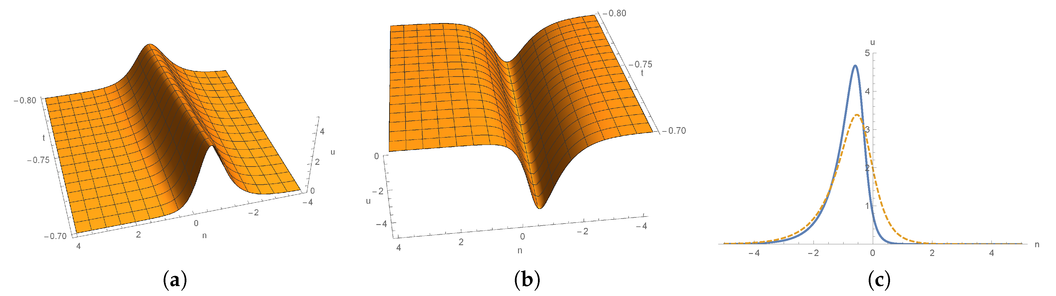
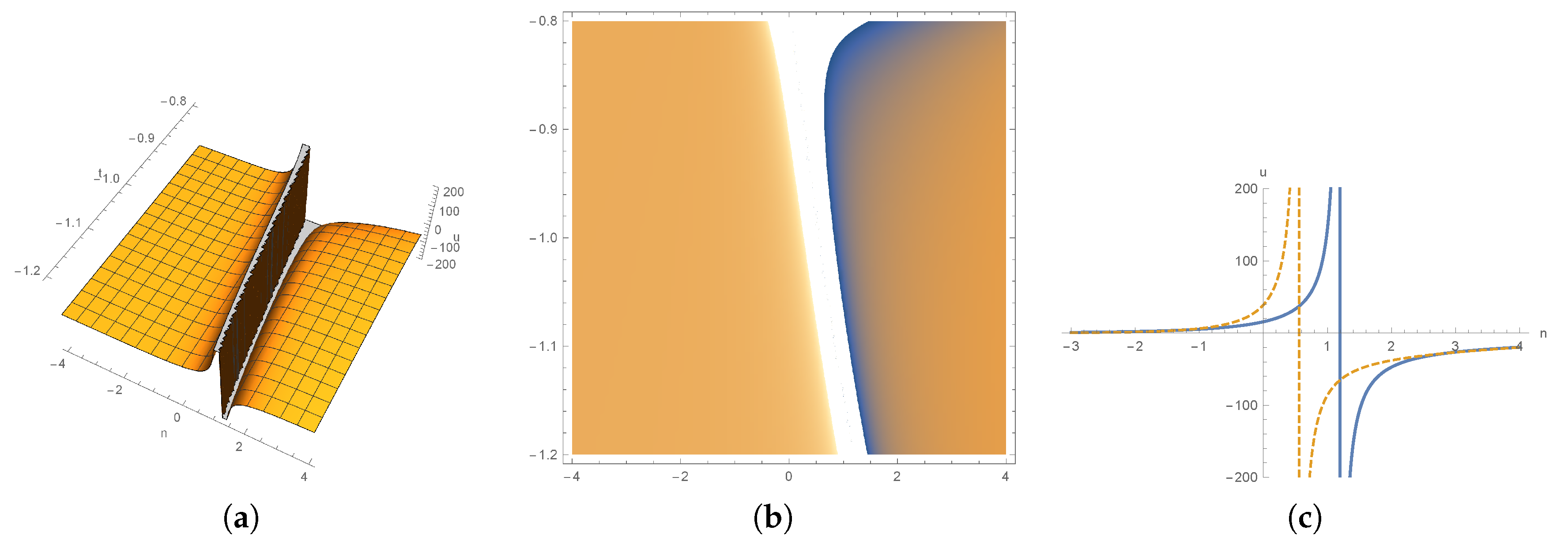
3. Dynamics of 1-Soliton Solution and 2-Soliton Solutions

To proceed, we consider the expressions of functions $k_j$ $l_j$, ${\omega }_j$ and ${\sigma }_j$. For the first equation in (22a), one can find that $-k_j$ is a solution if $k_j$ is a solution. By solving the differential Equations (22a) and (22b), we immediately have

$$\begin{array}{cc}\hfill & k_j=ln\left(\frac{1+e^{2t+c_j}}{1-e^{2t+c_j}}\right),{\omega }_j=\frac{{\alpha }_j{e}^{t+2c_j}}{(1-e^{2t+c_j})\sqrt{1-e^{4t+2c_j}}},\hfill \end{array}$$

(24a)

$$\begin{array}{cc}\hfill & l_j=ln\left(\frac{1+e^{2t+d_j}}{1-e^{2t+d_j}}\right),{\sigma }_j=\frac{{\beta }_j{e}^{3t+2d_j}}{(1-e^{2t+d_j})\sqrt{1-e^{4t+2d_j}}},\hfill \end{array}$$

(24b)

where $c_j,d_j\in \mathbb{R}$ and ${\alpha }_j,{\beta }_j\in \mathbb{R}\backslash \left\{0\right\}$ $(j=1,2,\dots ,N)$ are real constants. Here, ${\alpha }_j$ and ${\beta }_j$ play the role of phase shifts. One has to assume that $t<min\{-\frac{c_j}{2},-\frac{d_j}{2}\}$ in order to guarantee the real properties of $k_j$ $l_j$, ${\omega }_j$ and ${\sigma }_j$. Under the condition $t<min\{-\frac{c_j}{2},-\frac{d_j}{2}\}$, one knows that $k_j>0$ and $l_j>0$. In addition, one can recognize that $k_j,{\omega }_j\to +\infty$ as $t\to -\frac{c_j}{2}$ and $k_j,{\omega }_j\to 0$ as $t\to -\infty$. Similar results also hold for functions $l_j$ and ${\sigma }_j$.

We now consider the dynamical properties of 1-soliton solution (16) and 2-soliton solutions (20). Without loss of generality, we only focus on the dynamics of $u_n$, since $v_n$ behaves similarly. We first pay attention to $u_n$ in (16). For the sake of brevity, we denote ${\omega }_1=sgn\left({\alpha }_1\right)e^{{\rho }_1}$ and ${\sigma }_1=sgn\left({\beta }_1\right)e^{{\varrho }_1}$, i.e.,

$$\begin{array}{}\hfill (25\mathrm{a})& {\rho }_1=t+2c_1-ln\left((1-e^{2t+c_1})\sqrt{1-e^{4t+2c_1}}\right)+ln\left|{\alpha }_1\right|,\hfill \hfill (25\mathrm{b})& {\varrho }_1=3t+2d_1-ln\left((1-e^{2t+d_1})\sqrt{1-e^{4t+2d_1}}\right)+ln\left|{\beta }_1\right|.\hfill \end{array}$$

Then, we can rewrite $u_n$ (16) as

$$\begin{array}{c}\hfill u_n=\{\begin{array}{cc}\frac{\mathrm{sgn}\left({\alpha }_1\right)}{2}{e}^{\frac{{\xi }_1+{\rho }_1-({\eta }_1+{\varrho }_1+{\theta }_{11})}{2}}\mathrm{sech}\frac{{\xi }_1+{\eta }_1+{\rho }_1+{\varrho }_1+{\theta }_{11}}{2},\hfill & {\alpha }_1{\beta }_1<0,\hfill \\ \frac{\mathrm{sgn}\left({\alpha }_1\right)}{2}{e}^{\frac{{\xi }_1+{\rho }_1-({\eta }_1+{\varrho }_1+{\theta }_{11})}{2}}\mathrm{csch}\frac{{\xi }_1+{\eta }_1+{\rho }_1+{\varrho }_1+{\theta }_{11}}{2},\hfill & {\alpha }_1{\beta }_1>0.\hfill \end{array}\end{array}$$

(26)

For ${\alpha }_1{\beta }_1<0$, $u_n$ is nonsingular and provides a solitary wave because of the soliton part $sech\frac{{\xi }_1+{\eta }_1+{\rho }_1+{\varrho }_1+{\theta }_{11}}{2}$. Moreover, the part $\frac{sgn\left({\alpha }_1\right)}{2}{e}^{\frac{{\xi }_1+{\rho }_1-({\eta }_1+{\varrho }_1+{\theta }_{11})}{2}}$ defines a time varying amplitude due to the nonisospectral effect. In terms of the sign of parameter ${\alpha }_1$, the amplitude of the wave can be positive or negative, which corresponds to soliton or anti-soliton. The top trace is given by the point trace

$$\begin{array}{c}\hfill n\left(t\right)=-\frac{{\rho }_1+{\varrho }_1+{\theta }_{11}}{k_1+l_1}.\end{array}$$

(27)

Furthermore,

$$\begin{array}{c}\hfill \frac{dn\left(t\right)}{dt}=(\mathrm{csch}(2t+c_1)+\mathrm{csch}(2t+d_1))\frac{k_1+l_1-2({\rho }_1+{\varrho }_1+{\theta }_{11})}{{(k_1+l_1)}^2}\end{array}$$

(28)

implies the time-varying velocity of the wave. We illustrate this soliton in Figure 1.

It is worth noting that this soliton is not in a symmetric shape when $c_1\ne d_1$. This is because, for any fixed t,

$$\begin{array}{c}\hfill u_n\sim \{\begin{array}{cc}O\left(\mathrm{s}\mathrm{g}\mathrm{n}(-{\beta }_1)e^{-l_{1}n}\right),\hfill & n\to +\infty ,\hfill \\ O\left(\mathrm{s}\mathrm{g}\mathrm{n}\left({\alpha }_1\right)e^{k_{1}n}\right),\hfill & n\to -\infty .\hfill \end{array}\end{array}$$

(29)

This phenomenon is very similar to the solitons’ behavior of negative order AKNS equation [33].

For ${\alpha }_1{\beta }_1>0$, $u_n$ has singularity along the point trace (27) and the velocity is still expressed by (28). We depict this solution in Figure 2.

We next focus on $u_n$ given by (20). Since $k_j,l_j,{\omega }_j$ and ${\sigma }_j$$(j=1,2)$ are functions of t, it is intractable to make asymptotic analysis as usual [34]. Here, we only depict $u_n$ in Figure 3.

4. Multisoliton Solutions for nsd-mKdV Equation (4) and Dynamics

The nsd-mKdV Equation (4) can be derived from the nsd-AKNS Equation (3) by imposing constraint $v_n=ϵu_n$, while it is difficult to derive its soliton solutions by imposing constraint $h_n=ϵg_n$ since there is no linear relation between ${\omega }_j$ and ${\sigma }_j$. This can be demonstrated by the 1-soliton solution.

To derive the multisoliton solutions for the nsd-mKdV Equation (4), we take the dependent variable transformation

$$\begin{array}{c}\hfill u_n=\frac{g_n}{f_n},\end{array}$$

(30)

which yields the bilinear form for Equation (4)

$$\begin{array}{}\hfill (31\mathrm{a})& D_t{g}_n·f_n=\frac{1}{2}\left((2n+3)g_{n+1}{f}_{n-1}-(2n-1)g_{n-1}{f}_{n+1}\right),\hfill \hfill (31\mathrm{b})& f_n^2-f_{n+1}{f}_{n-1}=ϵg_n^2.\hfill \end{array}$$

Analogous to the previous analysis, one can successively derive 1-soliton, 2-soliton, and N-soliton solutions. The N-soliton solutions are given by

$$\begin{array}{cc}\hfill f_{n,N}=& \sum _{\kappa =0,1}{A}_1\left(\kappa \right)exp\left({\displaystyle \sum _{j=1}^{2N}}{\kappa }_j({\xi }_j+ln{\varpi }_j)+{\displaystyle \sum _{1\le j<s}^{2N}}{\kappa }_j{\kappa }_s{\vartheta }_{js}\right),\hfill \end{array}$$

(32a)

$$\begin{array}{cc}\hfill g_{n,N}=& \sum _{\kappa =0,1}{A}_2\left(\kappa \right)exp\left({\displaystyle \sum _{j=1}^{2N}}{\kappa }_j({\xi }_j+ln{\varpi }_j)+{\displaystyle \sum _{1\le j<s}^{2N}}{\kappa }_j{\kappa }_s{\vartheta }_{js}\right),\hfill \end{array}$$

(32b)

where ${\xi }_{N+j}={\xi }_j,{\varpi }_{N+j}={\varpi }_j$ and

$$\begin{array}{}\hfill (33\mathrm{a})& k_{j,t}=2sinh{k}_j,{\varpi }_{j,t}=\left(2cosh{k}_j+sinh{k}_j\right){\varpi }_j,(j=1,2,\dots ,N),\hfill \hfill (33\mathrm{b})& e^{{\vartheta }_{j(N+s)}}=-\frac{ϵ}{4}{\mathrm{csch}}^2\frac{k_j+k_s}{2},(j,s=1,2,\dots ,N),\hfill \hfill (33\mathrm{c})& e^{{\vartheta }_{(N+j)(N+s)}}=e^{{\vartheta }_{js}}=-4ϵ{sinh}^2\frac{k_j-k_s}{2},(1\le j<s\le N),\hfill \end{array}$$

and $A_1\left(\kappa \right)$ and $A_2\left(\kappa \right)$ are defined by (23).

Equation (33a) gives rise to $k_j$ (24a) and

$$\begin{array}{c}\hfill {\varpi }_j=\frac{{\alpha }_j{e}^{2(t+c_j)}}{(1-e^{2t+c_j})\sqrt{1-e^{4t+2c_j}}},c_j\in \mathbb{R},{\alpha }_j\in \mathbb{R}\backslash \left\{0\right\}.\end{array}$$

(34)

Similarly, it is necessary to take $t<-\frac{c_j}{2}(j=1,2,\dots ,N)$. In terms of (25a), the 1-soliton solution can be expressed as

$$\begin{array}{c}\hfill u_n=\{\begin{array}{cc}sinh{k}_1\mathrm{sech}({\xi }_1+{\rho }_1+t-ln(2sinh{k}_1)),\hfill & ϵ=-1,\hfill \\ sinh{k}_1\mathrm{csch}({\xi }_1+{\rho }_1+t-ln(2sinh{k}_1)),\hfill & ϵ=1.\hfill \end{array}\end{array}$$

(35)

Obviously, solution (35) is nonsingular when $ϵ=-1$ and has singularity when $ϵ=1$. For $ϵ=-1$, (35) provides a solitary wave with time varying amplitude $sinh{k}_1$. The top trace is given by the point trace

$$\begin{array}{c}\hfill n\left(t\right)=\frac{1}{k_1}(ln(2sinh{k}_1)-{\rho }_1-t),\end{array}$$

(36)

and the velocity is

$$\begin{array}{c}\hfill \frac{dn\left(t\right)}{dt}=\mathrm{csch}(2t+c_1)\frac{k_1-2({\rho }_1+t-ln(2sinh{k}_1))}{k_1^2}.\end{array}$$

(37)

For $ϵ=1$, (35) has singularity along with point trace (36) and the velocity is still given by (37).

Figure 4a,c depict the solution (35) with $ϵ=-1$ and $ϵ=1$, respectively. Figure 4b shows the symmetric shape and the Gaussian-distributed structure with respect to n for a given t. Figure 4d exhibits the movement of the singularity point.

The 2-soliton solutions for nsd-mKdV Equation (4) read

$$\begin{array}{c}\hfill u_n=\frac{g_n}{f_n},\end{array}$$

(38)

in which

$$\begin{array}{}\hfill (39\mathrm{a})& g_n={\varpi }_1{e}^{{\xi }_1}+{\varpi }_2{e}^{{\xi }_2}-ϵ{\varpi }_1^2{\varpi }_2{e}^{2{\xi }_1+{\xi }_2+{\varsigma }_1+{\varsigma }_{12}+{\mu }_{12}}-ϵ{\varpi }_1{\varpi }_2^2{e}^{{\xi }_1+2{\xi }_2+{\varsigma }_{12}+{\varsigma }_2+{\mu }_{12}},\hfill \hfill (39\mathrm{b})& f_n=1-ϵ{\varpi }_1^2{e}^{2{\xi }_1+{\varsigma }_1}-2ϵ{\varpi }_1{\varpi }_2{e}^{{\xi }_1+{\xi }_2+{\varsigma }_{12}}-ϵ{\varpi }_2^2{e}^{2{\xi }_2+{\varsigma }_2}+{\varpi }_1^2{\varpi }_2^2{e}^{2{\xi }_1+2{\xi }_2+{\varsigma }_1+2{\varsigma }_{12}+{\varsigma }_2+2{\mu }_{12}},\hfill \end{array}$$

where $k_j$, ${\varpi }_j$ ($j=1,2$) and $e^{{\mu }_{12}}$ are given by (24a), (34) and (19c), respectively. In addition,

$$\begin{array}{c}\hfill {\varsigma }_1=-2ln(2sinh{k}_1),{\varsigma }_2=-2ln(2sinh{k}_2),{\varsigma }_{12}=-2ln\left(2sinh\frac{k_1+k_2}{2}\right).\end{array}$$

(40)

When $ϵ=-1$, solution (38) is nonsingular. Figure 5 and Figure 6 depict soliton–soliton interaction, respectively, and soliton–anti-soliton interaction of the nsd-mKdV Equation (4) with $ϵ=-1$.

When $ϵ=1$, solution (38) has singularity, which appears at the point trace

$$\left\{(n,t)\right|1+{\varpi }_1^2{\varpi }_2^2{e}^{2{\xi }_1+2{\xi }_2+{\varsigma }_1+2{\varsigma }_{12}+{\varsigma }_2+2{\mu }_{12}}={\varpi }_1^2{e}^{2{\xi }_1+{\varsigma }_1}+2{\varpi }_1{\varpi }_2{e}^{{\xi }_1+{\xi }_2+{\varsigma }_{12}}+{\varpi }_2^2{e}^{2{\xi }_2+{\varsigma }_2}\}.$$

Figure 7 and Figure 8 depict soliton–soliton interaction, respectively, soliton–anti-soliton interaction of the nsd-mKdV Equation (4) with $ϵ=1$.

5. Conclusions

In this paper, we have discussed the multisoliton solutions for nsd-AKNS Equation (3) by applying the Hirota’s method. Dynamical behaviors for some obtained soliton solutions are identified through asymptotic analysis. In terms of the sign of product ${\alpha }_1{\beta }_1$, we present two kinds of 1-soliton solution for nsd-AKNS Equation (3). One is nonsingular and the other is singular. Nonisospectral effects on amplitude, top trace/singularity point trace, and velocity of these two 1-soliton solutions are analyzed emphatically. The nonsingular 1-soliton exhibits a nonsymmetric structure when $c_1\ne d_1$. Since functions $k_j,l_j,{\omega }_j$ and ${\sigma }_j$$(j=1,2)$ depend on t, the asymptotic analysis on 2-soliton solutions to nsd-AKNS Equation (3) is not given in the present paper. With the help of Hirota’s method, we also present the multisoliton solutions to the nsd-mKdV Equation (4). For the plus type nsd-mKdV Equation (4) ($ϵ=-1$), the resulting multisoliton solutions are nonsingular, while, for the minus type nsd-mKdV Equation (4) ($ϵ=1$), the resulting multisoliton solutions are singular. Although the multisoliton solutions to the nsd-mKdV Equation (4) have appeared in Refs. [27,28], there is little description on the dynamics of 1-soliton solutions. To understand the 2-soliton solutions better, we give some figures. The detailed discussion on the applications of the graphs will be given in the near future. We hope that the results given in this article might attract some attention in the areas of semi-discrete integrable system and nonisospectral integrable system. Particularly, this work will be beneficial to developing other approaches to study the multi-component nonisospectral semi-discrete integrable system.

References

1. Chen, H.; Liu, C.S. Solitons in nonuniform media. Phys. Rev. Lett. 1976, 37, 693–697. [Google Scholar] [CrossRef]
2. Hirota, R.; Satsuma, J. N-soliton solution of the KdV equation with loss and nonuniformity terms. J. Phys. Soc. Jpn. 1976, 41, 2141–2142. [Google Scholar] [CrossRef]
3. Calogero, F.; Degasperis, A. Conservation laws for classes of nonlinear evolution equations solvable by the spectral transform. Commun. Math. Phys. 1978, 63, 155–176. [Google Scholar] [CrossRef]
4. Ma, W.X. An approach for constructing nonisospectral hierarchies of evolution equations. J. Phys. A Gen. Math. 1992, 25, L719–L726. [Google Scholar] [CrossRef]
5. Ma, W.X. The algebraic structure of zero curvature representations and application to coupled KdV systems. J. Phys. A Gen. Math. 1993, 26, 2573–2582. [Google Scholar] [CrossRef]
6. Ma, W.X. A simple scheme for generating nonisospectral flows from the zero curvature representation. Phys. Lett. A 1993, 179, 179–185. [Google Scholar] [CrossRef]
7. Fuchssteiner, B. Master symmetries, higher order time-dependent symmetries and conserved densities of nonlinear evolution equations. Prog. Theor. Phys. 1983, 70, 1508–1522. [Google Scholar] [CrossRef] [Green Version]
8. Ma, W.X.; Fuchssteiner, B. Algebraic structure of discrete zero curvature equations and master symmetries of discrete evolution equations. J. Math. Phys. 1999, 40, 2400–2418. [Google Scholar] [CrossRef] [Green Version]
9. Gupta, M.R. Exact inverse scattering solution of a nonlinear evolution equation in a nonuniform media. Phys. Lett. A 1979, 72, 420–422. [Google Scholar] [CrossRef]
10. Burtsev, S.P.; Zakharov, V.E.; Mikhailov, A.V. Inverse scattering method with variable spectral parameter. Theor. Math. Phys. 1987, 70, 227–240. [Google Scholar] [CrossRef]
11. Zhang, D.J.; Chen, D.Y. Negatons, positons, rational-like solutions and conservation laws of the KdV equation with loss and nonuniformity terms. J. Phys. A Gen. Math. 2004, 37, 851–865. [Google Scholar] [CrossRef] [Green Version]
12. Zhao, S.L.; Zhang, D.J.; Chen, D.Y. N-soliton solutions of non-isospectral derivative nonlinear Schrödinger equation. Chin. Phys. Lett. 2009, 26, 030202. [Google Scholar]
13. Silem, A.; Zhang, C.; Zhang, D.J. Dynamics of three nonisospectral nonlinear Schrödinger equations. Chin. Phys. B 2019, 28, 020202. [Google Scholar] [CrossRef]
14. Eilbeck, J.C.; Lomdah, P.S.; Scott, A.C. The discrete self-trapping equation. Physica D 1985, 16, 318–338. [Google Scholar] [CrossRef]
15. Laedke, E.W.; Spatschek, K.H.; Turitsyn, S.K. Stability of discrete solitons and quasicollapse to intrinsically localized modes. Phys. Rev. Lett. 1994, 73, 1055–1059. [Google Scholar] [CrossRef]
16. Cao, C.W.; Zhang, G.Y. Integrable symplectic maps associated with the ZS-AKNS spectral problem. J. Phys. A Math. Theor. 2012, 45, 265201. [Google Scholar] [CrossRef]
17. Xue, L.L.; Liu, Q.P. A supersymmetric AKNS problem and its Darboux-Bäcklund transformations and discrete systems. Stud. Appl. Math. 2015, 135, 35–62. [Google Scholar] [CrossRef] [Green Version]
18. Zhao, S.L. A discrete negative AKNS equation: Generalised Cauchy matrix approach. J. Nonlinear Math. Phys. 2016, 23, 544–562. [Google Scholar] [CrossRef] [Green Version]
19. Chen, K.; Deng, X.; Zhang, D.J. Symmetry constraint of the differential-difference KP hierarchy and a second discretization of the ZS-AKNS system. J. Nonlinear Math. Phys. 2017, 24, 18–35. [Google Scholar] [CrossRef] [Green Version]
20. Zhao, S.L.; Shi, Y. Discrete and semidiscrete models for AKNS equation. Z. Naturforsch. A 2017, 72, 281–290. [Google Scholar] [CrossRef]
21. Zhao, S.L. Discrete potential Ablowitz–Kaup–Newell–Segur equation. J. Differ. Equ. Appl. 2019, 25, 1134–1148. [Google Scholar] [CrossRef]
22. Ablowitz, M.J.; Ladik, J.F. Nonlinear differential-difference equations. J. Math. Phys. 1975, 16, 598–603. [Google Scholar] [CrossRef]
23. Ablowitz, M.J.; Prinari, B.; Trubatch, A.D. Discrete and Continuous Nonlinear Schrödinger Systems; Cambridge University Press: Cambridge, UK, 2004. [Google Scholar]
24. Ablowitz, M.J.; Kaup, D.J.; Newell, A.C.; Segur, H. Nonlinear-evolution equations of physical significance. Phys. Rev. Lett. 1973, 31, 125–127. [Google Scholar] [CrossRef]
25. Zhang, D.J.; Ning, T.K.; Bi, J.B.; Chen, D.Y. New symmetries for the Ablowitz–Ladik hierarchies. Phys. Lett. A 2006, 359, 458–466. [Google Scholar] [CrossRef] [Green Version]
26. Zhang, D.J.; Chen, S.T. Symmetries for the Ablowitz–Ladik hierarchy: II. Integrable discrete nonlinear Schrödinger equations anddiscrete AKNS hierarchy. Stud. Appl. Math. 2010, 125, 419–443. [Google Scholar] [CrossRef]
27. Li, Q.; Chen, D.Y.; Zhang, J.B.; Chen, S.T. Solving the non-isospectral Ablowitz–Ladik hierarchy via the inverse scattering transform and reductions. Chaos Soliton Fractals 2012, 45, 1479–1485. [Google Scholar] [CrossRef]
28. Li, Q.; Duan, Q.Y.; Zhang, J.B. Soliton solutions of the mixed discrete modified Korteweg Cde Vries hierarchy via the inverse scattering transform. Phys. Scr. 2012, 86, 065009. [Google Scholar] [CrossRef]
29. Chen, S.T.; Chen, D.Y.; Li, Q.; Cheng, J.W. N-soliton-like and double Casoratian solutions of a nonisospectral Ablowitz–Ladik equation. Int. J. Mod. Phys. B 2016, 30, 1640008. [Google Scholar] [CrossRef]
30. Chen, X.M.; Chang, X.K.; Su, J.Q.; Hu, X.B.; Yeh, Y.N. Three semi-discrete integrable systems related to orthogonal polynomials and their generalized determinant solutions. Nonlinearity 2015, 28, 2279–2306. [Google Scholar] [CrossRef]
31. Chen, X.M.; Hu, X.B.; Hoissen, F.M. Non-isospectral extension of the Volterra lattice hierarchy, and Hankel determinants. Nonlinearity 2018, 31, 4393–4422. [Google Scholar] [CrossRef] [Green Version]
32. Hirota, R. The Direct Method in Soliton Theory; Cambridge University Press: Cambridge, UK, 2004. [Google Scholar]
33. Zhang, D.J.; Ji, J.; Zhao, S.L. Soliton scattering with amplitude changes of a negative order AKNS equation. Physica D 2009, 238, 2361–2367. [Google Scholar] [CrossRef]
34. Hietarinta, J. Scattering of solitons and dromions. In Scattering: Scattering and Inverse Scattering in Pure and Applied Science; Pike, R., Sabatier, P., Eds.; Academic Press: London, UK, 2002; pp. 1773–1791. [Google Scholar]
Figure 1. Shape and motion of 1-soliton given by (26) for c 1 = 1 and d 1 = 1.35 . (a) soliton solution for α 1 = 1 and β 1 = 1 ; (b) anti-soliton solution for α 1 = 1 and β 1 = 1 ; (c) waves in blue (solid line) and yellow (dotted line) stand for plot (a) at t = 0.68 and t = 0.75 , respectively.
Mathematics 08 01889 g001
Figure 2. u n given by (26) for c 1 = 1.5 , d 1 = 0.01 , α 1 = 1 and β 1 = 1 . (a) shape and motion; (b) a contour plot of (a) with range n [ 4 , 4 ] and t [ 1.2 , 0.8 ] ; (c) waves in blue (solid line) and yellow (dotted line) stand for plot (a) at t = 1.2 and t = 1 , respectively.
Mathematics 08 01889 g002
Figure 3. 2-soliton solutions for u n with c 1 = 0.05 , c 2 = 0.06 , d 1 = 1 , d 2 = 1.2 , α 1 = α 2 = 0.1 and β 1 = β 2 = 0.1 . (a) shape and motion; (b) waves in blue (solid line) and yellow (dotted line) stand for plot (a) at t = 0.82 and t = 0.83 , respectively.
Mathematics 08 01889 g003
Figure 4. u n given by (35) for c 1 = 1 and α 1 = 1 . (a) shape and motion with ϵ = 1 ; (b) waves in blue (solid line) and yellow (dotted line) stand for plot (a) at t = 0.8 and t = 0.7 , respectively; (c) shape and motion with ϵ = 1 ; (d) waves in blue (solid line) and yellow (dotted line) stand for plot (c) at t = 1 and t = 0.6 , respectively.
Mathematics 08 01889 g004
Figure 5. u n given by (38) with ϵ = 1 for c 1 = 1 , c 2 = 0.4 and α 1 = α 2 = 1 . (a) shape and motion; (b) a contour plot of (a) with range n [ 10 , 20 ] and t [ 1.8 , 0.5 ] ; (c) waves in blue (solid line) and yellow (dotted line) stand for plot (a) at t = 0.8 and t = 1.2 , respectively.
Mathematics 08 01889 g005
Figure 6. u n given by (38) with ϵ = 1 for c 1 = 1 , c 2 = 0.6 , α 1 = 1 and α 2 = 1 . (a) shape and motion; (b) a contour plot of (a) with range n [ 10 , 20 ] and t [ 1.8 , 0.8 ] ; (c) waves in blue (solid line) and yellow (dotted line) stand for plot (a) at t = 1 and t = 0.8 , respectively.
Mathematics 08 01889 g006
Figure 7. u n given by (38) with ϵ = 1 for c 1 = 1 , c 2 = 0.8 and α 1 = α 2 = 1 . (a) shape and motion; (b) a contour plot of (a) with range n [ 5 , 15 ] and t [ 1.2 , 0.6 ] ; (c) waves in blue (solid line) and yellow (dotted line) stand for plot (a) at t = 1 and t = 0.8 , respectively.
Mathematics 08 01889 g007
Figure 8. u n given by (38) with ϵ = 1 for c 1 = 1 , c 2 = 0.8 , α 1 = 1 and α 2 = 1 . (a) shape and motion; (b) a contour plot of (a) with range n [ 10 , 20 ] and t [ 1.8 , 0.8 ] ; (c) waves in blue (solid line) and yellow (dotted line) stand for plot (a) at t = 1 and t = 1.2 , respectively.
Mathematics 08 01889 g008
Publisher’s Note: MDPI stays neutral with regard to jurisdictional claims in published maps and institutional affiliations.