Abstract
The shelf-space on which products are displayed is one of the most important resources in the retail environment. Therefore, decisions about shelf-space allocation and optimization are critical in retail operation management. This paper addresses the problem of a retailer who sells various products by displaying them on the shelf at stores. We present a practical shelf-space allocation model, based on a genetic algorithm, with vertical position effects with the objective of maximizing the retailer’s profit. The validity of the model is illustrated with example problems and compared to the CPLEX solver. The results obtained from the experimental phase show the suitability of the proposed approach.
1. Introduction
Shelf space is one of the scarcest resources in a retail store. While allocating shelf space, many retailers apply decision processes that result in a positive relationship between the amount of shelf space dedicated to a product and its sales.
Appropriate shelf-space assignment is one of the most critical factors in gaining an edge in the exceptionally competitive retail industry [1]. Despite the development of e-commerce, the traditional form of sale is still important. Even during the COVID-19 pandemic, customers continued to shop in traditional stores, especially in the food industry. Very large store assortment volumes pose an incredible challenge to retailers. Various shelf-space allocation models that assign a very large number of products to a shelf have been investigated over the years. The most frequent objective of such models is to maximize the retailer’s profit under certain limitations and promote rules in the store.
Karampatsa et al. [2] highlighted the importance of shelf-space allocation choices and their significance for analysts and retailers who aim to implement an appropriate decision-making process. Shelf-space assignment decisions include two components: the shelf space for a specific product category and the shelf space for a specific product in each product category [3].
A large number of different in-store categories are possible; therefore, there is growing interest in the impact of location characteristics at the category level. Both academics and practitioners agree that, depending on the location, product categories within a store may become more or less attractive to customers [4].
There are two main streams in which retailers can manipulate local category differences to improve store performance. First, there are efficient assortment strategies, i.e., offering various assortments in different stores, adjusted to local needs. Second, there is the efficient allocation of scarce shelf-space resources, i.e., the assignment of shelf space available at each outlet to different product categories. Obviously, efficient allocation of promotional budgets, local personnel, and store shelf space needs to be adjusted by the retailers on a store-level basis [4,5].
Retailers generally believe that product characteristics and retailing factors influence sales and stimulate the consumer to make impulse purchases. According to Kacen et al. [6], the retail factor that has the greatest influence on impulse buying is a store environment with a high–low pricing strategy. They suggested that retailers execute promotional tactics and implement appropriate merchandising rules in order to attract consumers’ attention and encourage impulse buying [6].
Visual merchandising has a great role in the effective management of retail brand preferences and communication strategies. It characterizes retail brands by social likeness and associations. The supporting factors of a visual merchandising cognition scale are in-fashion, attractiveness, and function. Friendly attitudes of approving customers toward visual merchandising have positive effects on purchase intentions. Brand recognition is highly influenced by the cognitive representation of the retail environment [7].
Retailers have come a long way in creating suitable plans for distributing store shelf space to product categories. However, there remains room for various improvements. While shelf-space allocation models incorporate complex interactions of different variables, existing approaches do not fully account for all store perspectives [8].
The main goal of this article is to develop a retail shelf-space allocation model that is relevant to practice and propose genetic algorithms that can be applied by category managers to solve it. Several of our contributions to addressing the considered shelf-space allocation problem (SSAP) can be summarized as follows:
- As visual merchandising is a critical issue for category managers, our model includes vertical and horizontal category grouping rules that make planograms more attractive to customers.
- To the best of our knowledge, this is the first proposal of an SSAP model that includes not only facings but also capping (which means placing a product on top of another one, where rotation of the top product is allowed) and nesting (which means placing a product underneath another one, such as a basket or plate).
- Generally speaking, cheaper products should be located on bottom shelves, but luxury products should be located at the customer’s eye level, on the top shelves [9]. However, the limitation of the existing mathematical SSAP approaches is that it neglects merchandising rules based on product price categories, which means that products should be placed on different vertical shelf levels based on their price.
- In the developed retail SSAP model, four groups of constraints are simultaneously considered, which allows it to analyze retailers’ locations and practical pricing rules at the same time. We present constraints according to the following types: shelf constraints, product constraints, multi-shelf constraints, and category constraints.
- We implemented a genetic algorithm and performed experiments on relevant practical problem sizes. The quality of the proposed solution was estimated using the CPLEX solver. In the designed algorithm, we paid special attention to the newly proposed improvement method, which can be valuable for category managers while creating either manual or automatic planograms.
The remainder of this paper is organized as follows. Section 2 summarizes the analysis of related works. In Section 3, the definition of the problem is given. Section 4 presents the mathematical model for both profit maximization problems. In Section 5, solution procedures based on a genetic algorithm are described. The results of computational experiments are reported in Section 6, and conclusions are provided in Section 7.
2. Related Works
The shelf-space allocation problem has been analyzed in many studies, as it affects retail operations and store organization. In this section, we provide an overview of published research results in two domains of interest to our research. The first research literature stream relates to customers’ visual attention to the product in the store. Given our interest in optimal shelf-space implications, an overview of the relevant shelf-space allocation literature is provided in the second part of this review.
2.1. Visual Attention to the Product
Retailers try to attract customers, secure more traffic in their stores, and increase sales. Therefore, they explore different strategies to perform these tasks, such as creating a good visual display, which encourages impulse sales, putting the best product at the front of the store, decorating shelves, and so on. In our opinion, retailers should include visual product cases, traffic flow, and overall store layout into their merchandising rules for adjusting shelf space.
Many customers choose what to buy when they are already inside the store. They often prefer not to choose the cheapest product from the defined category, but the decisive factors usually include product quality, loyalty to a specific brand, brand notoriety, willingness to try something new, and other marketing factors that affect their choice [3]. Through fitting promotion tactics, the retailer attempts to obtain greater benefit from customers when they visit the store.
Djamasbi et al. [10] emphasized the factors that influence customers’ visual attention. He noted that bigger products are more discernible than small ones. The same applies to products with brighter colors, which seem to be more appealing to customers than darker ones. Products displayed on eye-level shelves attract more attention than those found on lower shelves.
Ngo and Byrne [11] noted that customers glanced at shelves from the top left to the bottom right corner following a Z-shaped path. How products are displayed on store shelves attracts customers’ attention to a greater or lesser degree. Products that generate social endorsement, fulfillment, self-expression, the acknowledgment of being special, and intellectual inspiration inspire incredible involvement from customers [12].
Huang et al. [13] illustrated the positive effect of product promotions. Because of the vast potential of promotions, customers become more loyal to a particular product, investing more time in front of the shelf and effectively analyzing the product, which results in carefully made purchase decisions. According to Desrochers and Nelson [14], customer buying decisions can have immense impacts if they are used to fortify suitable product classification and prior product allocation to another subcategory. Anic, Radas, and Lim [15] suggested that customers’ buying behaviors are influenced by the store layout and traffic paths, which are critical determinants toward the store appeal.
The goal of shelf merchandising is to efficiently organize in-store merchandising rules and to allocate products to the right shelves to increase sales. Shelf merchandising of regional products in stores includes principles to make regional products visible and accessible to customers by assigning them enough shelf space. Lombart et al. [16] highlighted the superior performance of visual merchandising of regional products within their product categories. They proposed a strategy to increase the visibility of such products, develop customers’ positive perception toward them, and improve the retailer’s local image.
In-store merchandising of child-targeted products includes strategizing the allocation of products to shelves at children’s eye level, creating colorful packaging and product promotions, and preparing ample shelf space for products dedicated to children [17]. Special displays and price promotions are more effective than increasing shelf space dedicated to products.
Appropriate merchandising rules are the key driver of visual attention to a planogram in a retail store. Within the retail industry, merchandising is the action of promoting products to stimulate their sales.
2.2. Shelf-Space Allocation
Category management is an amazingly competitive field in retail. Different tactics are utilized to impact customer purchases. These incorporate product assortment, store location and organization, floor and space planning, pricing strategies, promotion actions, assortment planning, advertising, etc. [18]. The goal of retailers is to maximize benefits from product sales, regardless of the brand. They must assign their limited shelf space in the best way possible according to practical verification [19].
The retailer’s standard work lies in successive decisions with respect to the following issues: assortment size determination, allocation of products to shelves, specification of prices and discounts, and managing in-store shelf replenishment. Retail shelf management includes rapid and cost-effective operations involving retail tasks and client requests [20]. Hübner and Schaal ([19,21]) investigated the matching of assortment and shelf-space planning decisions with regard to the stochastic and space-elastic demand and out-of-assortment and out-of-stock substitution effects. Schaal and Hübner [22] collected practical guidelines concerning the impact of cross-space elasticities and product substitutions on shelf-space decisions, which are very useful for retailers. Karampatsa et al. [2] presented the goal function of demand by incorporating inventory level-dependent decisions. They differentiated between backroom and showroom inventories. Hübner and Schaal [23] presented a shelf-space optimization model that included in-store replenishment rules. They concluded that the demand increases if there is more shelf space allocated to products because it leads to higher product visibility. Obviously, the costs of replenishment decrease, but the inventory costs increase.
Merchandising tactics incorporate ways to expose products in stores as well as allow for their free testing, distribute showcasing materials, deliver on-the-spot demonstrations, and provide special offers or regular promotions. The successful merchandiser must decide on which fixture types, on which shelves, and in which positions the product will be shown. Typically, this is a very difficult assignment because inaccurate product allocation negatively influences store sales [24].
In their research on shelf space, Hübner and Schaal [19] concluded that a retailer could increase sales and profits by using better strategies to manage existing shelf space. Assuming that retailers can increase sales by improving product exposition and shelf-space allocation, they proposed two different ways to improve the profits gained by retailers: by adapting the shelf space to the product’s movement on planograms and by reorganizing products.
Another technique with which retailers can increase product sales is to prepare engaging shelf displays by determining the ideal product position within planogram shelves. Among the factors that influence sales are horizontal positioning, vertical positioning, product adjacencies, and category arrangement [25]. Bianchi-Aguiar et al. [26] proposed grouping the products into families and organizing them into rectangular shapes to form hierarchical structural subcategories.
Shelf-space allocation decisions are of critical importance in a retail store. Because of this, a considerable number of studies have stressed that the space allocated to a product category has a positive effect on category performance ([2,8]). Chen et al. [27] emphasized that assigning space to a product category has a double effect, as it attracts customers to the store and has a positive influence on the sales of this category as well as other categories when customers are in the store. Karampatsa et al. [2] highlighted that the space allocated to a category has a positive effect on category performance and results in increased visibility of products. Moreover, the category with increased shelf space competes with other categories for customer loyalty [5].
Evidence suggests that many retailers may not have a correct understanding of the influence of shelf design on consumers’ shopping behaviors. For example, retailers and consumers have a different expectation of product positioning on shelves. In consumers’ opinions, retailers order products according to criteria such as price, popularity, and promotional status. However, in turn, retailers and manufacturers do not take into account consumers’ needs and expectations for product allocation. They believe that consumers expect retailers to allocate popular brands to the center of the shelf, but in a real store, retailers do not place such products in these central positions. Customers can find these branded products at the end of an aisle, which, according to retailers, results in more time spent on finding and investigating the desired product [28].
3. Problem Definition
This study deals with the problem faced by a retailer who sells various products within a category and displays them on limited shelf space. We aim to determine on which shelf to place the product and what amount of shelf space to allocate to each product in order to maximize the retailer’s total profit. Shelf-space allocation is focused on two factors when considered by retailers. On the one hand, they must display products on the right shelves. On the other hand, customer satisfaction and product demand are influenced by the proximity of similar products and by the location on the shelf where products are placed on a planogram. Planograms are a graphic illustration of products’ allocation on store shelves to help the retailer determine the appropriate position of the product on the shelf and its number of facings. Figure 1 shows an example of a planogram that has 10 products on three shelves in two vertical segments.
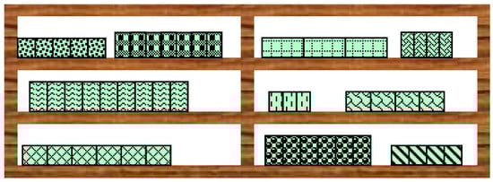
Figure 1.
An example of a planogram.
To model the problem, we introduce the following variables and parameters. In this research, subscripts are used as variables’ indexes, and superscripts are used for the explanation of mnemonics (they are not treated as indexes or powers).
Parameters and indices:
- —total number of categories;
- —total number of subcategories;
- —total number of shelves;
- —total number of products;
- —category index, ;
- —subcategory index, ;
- —shelf index, ;
- —product index, .
Parameters of category :
- —minimum category size as a percentage of the shelf length.
Parameters of shelf :
- —length;
- —depth;
- —height.
Parameters of product :
- —width;
- —depth;
- —height;
- —supply limit;
- —unit profit;
- —category;
- —subcategory;
- —nesting height, , or if the product cannot be nested;
- —front orientation binary parameter;
- —side orientation binary parameter;
- —cluster;
- —minimum number of facings;
- —maximum number of facings;
- —maximum number of caps per group of facings;
- —maximum number of nests of one facing;
- —minimum number of shelves to which the product can be allocated;
- —maximum number of shelves to which the product can be allocated;
Decision variables:
- ;
- —the number of product facings;
- —the number of product caps;
- —the number of product nets;
- ;
- .
The SSAP can be formulated as follows. There is a given number of products that are assigned to categories and price subcategories. These products must be displayed on shelves of a planogram. The retailer defines the minimum possible size of the category on the planogram to make the products of the category sufficiently visible. Generally, the categories are vertical; i.e., the products of one category are grouped on a planogram. The price subcategories are assigned to the shelves as well as to the products. This means that the price subcategories are horizontal, so the higher the product price (or the more branded the product is), the closer it is to the customer’s eye-level. Conversely, the lower the product price (or the more demanded it is), the lower it is placed, but it can also be placed on any higher shelf. According to merchandising rules, expensive products cannot be placed on lower shelves. The problem is finding the appropriate shelf space for each product, thus maximizing the retailer’s profit.
Figure 2 shows the rules of allocating products to vertical categories A, B, and C and numeric price subcategories on the planogram. The darker the color of the category, the more expensive the product is, so they cannot be allocated to the lower shelves. In contrast, cheaper products have light colors; they can be allocated to lower and upper shelves (at eye-level). The products with medium–light colors must be allocated to no lower than the middle shelf. Products of the same category must be grouped and located together in their vertical category on the planogram.
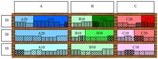
Figure 2.
Allocation of the categories and price subcategories on the planogram.
Similar products within one category with complementary characteristics, functions, or tastes can be grouped into clusters and placed adjacently on the same shelf. This merchandising rule is used to ensure the substitution effect between complementary products when one of them is out of stock. On the shelf, the product can be placed in a front orientation (for which width is taken as a line parameter) or side orientation (for which depth is taken as a line parameter).
In this research, the product quantity parameter is not only facing because, in a real retail store, the product package can also be capped, nested, or neither capped nor nested. If the products’ packaging allows one product to be placed on top of a lower product in another rotated orientation, then it is called capping. Most rectangular boxes, such as boxes with teas or sweets, can be capped. In a real store, the capping can be rotated by 90–360 degrees, but because we investigated the planogram one-dimensionally, we considered only one possible orientation for capping. When the product’s packaging allows it to be placed inside another one, as in the case of bowls or plates, it is called nesting. Figure 3 and Figure 4 present the cap and nest allocation technique. It is assumed that in one front-orientated capped group, the number of facings is . For one side-orientated capped group, the number of facings is .
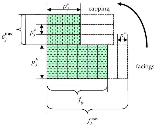
Figure 3.
Allocation of caps.
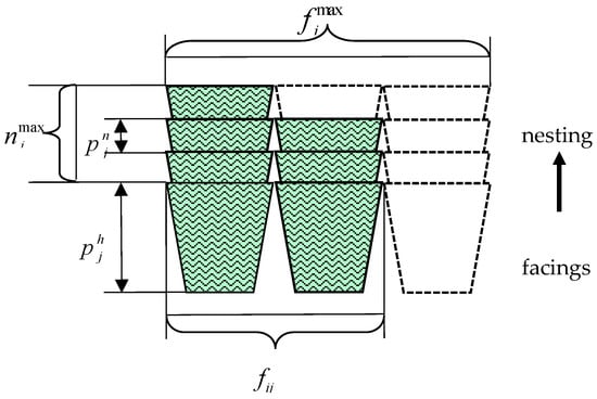
Figure 4.
Allocation of nests.
The parameter of the maximum possible caps in one capped group illustrates the situation in which too many caps are placed above the facings in a row, so products below may be damaged or destroyed, or capping products could fall off the shelf. A comparable effect is observed for nests: if too many nested products (bowls or plates) are placed inside the lower product on the shelf, the product below may be damaged or destroyed, or the upper product could fall off the shelf. The total number of product items comprises facings, caps, and nests.
The allocation is one-dimensional, so the following assumptions are introduced.
- Only one (top) row of facings with capping or nesting above it is investigated.
- Facings in the vertical dimension are not considered.
- A product supply limit applies to one top row of facings, including capping or nesting.
- The shelf depth applies to one top row of facings.
The aim is to find combinations of the number of facings , caps , and nests of a product that is allocated to shelf , subject to 4 types of constraints—shelf constraints, product constraints, multi-shelves constraints, and category constraints—in order to maximize profit obtained by the retailer.
4. Mathematical Models
Using the above notation, the SSAP model with the linear profit maximization function can be defined as follows:
Next, we present constraints that are used in both models.
4.1. Shelf Constraints
Shelf width:
Shelf depth:
Product height, including heights of caps and nests:
4.2. Product Constraints
Supply limit:
Minimum and maximum number of facings:
Maximum number of caps:
Maximum number of nests:
4.3. Multi-Shelf Constraints
Minimum and maximum number of shelves:
Front orientation is possible:
Side orientation is possible:
Only one orientation (front or side) is available:
The same product orientation on all shelves:
The next shelf only:
The same number of facings on all shelves:
The same cluster on the same shelf:
4.4. Category Constraints
The minimum category size if the products of this category exist on the shelf:
indicates a rounded value.
The possibility of allocating products based on their price subcategory:
4.5. Decision Variables
If the product exists on the shelf:
The number of facings:
The number of caps:
The number of nests:
If the product is placed in the front orientation:
If the product is placed in the side orientation:
5. Genetic Algorithm
In this section, we describe the proposed shelf-space allocation genetic algorithm. All of the components of the algorithm are briefly described below. Genetic algorithms (GAs) are meta-heuristics based on the evolutionary process of natural systems. Originally, they were applied to numerous optimization problems with sufficiently acceptable results. GAs are regularly seen as function optimizers, but the variety of problems to which GAs can be applied is extensive. Generally, a GA consists of the following elements: populations of chromosomes, selection according to the fitness function, crossover to produce new offspring, and random mutation in new offspring. The GA chromosomes commonly take the form of bit strings. Every chromosome (or individual) can be considered a locality in the search space of feasible candidate solutions. The defined fitness function scores each chromosome in the current population. The GA processes populations of chromosomes, progressively replacing one such population with another, taking the solution with a better fitness function to the next step. GA starts with the initial population. The simplest genetic operators include selection, single-point crossover, and mutation [29].
5.1. Solution Encoding and Crossover Operators
A candidate solution is represented as a string with a length equal to the number of products multiplied by the number of shelves. In detail, a candidate solution is represented by the chromosome in which each gene indicates whether a product is placed on the shelf and the number of units to be placed there. In such a chromosome, on each shelf, there is a place dedicated to each product, but if the constraints are not satisfied, the corresponding gene remains empty, and the product is allocated to another shelf. The population is represented as an array of individuals. In the proposed method, each gene consists of three parts: (1) true/false parameter—whether the product is allocated to the shelf; (2) numeric parameter—the number of facings of the product on the shelf; (3) numeric parameter—the number of caps or nests of the product on the shelf. Obviously, products may be either capped or nested or neither capped nor nested.
Standard genetic operators were developed in order to satisfy the above-mentioned constraints. In this algorithm, we adapted three recombination procedures:
- Two rankings [30]: ranks based on decreasing the total profit and decreasing the total free space on all shelves.
- Roulette wheel [30]: randomly chooses individuals for the crossover with a probability corresponding to its total profit.
- Tournament [31,32]: adopted binary tournament between two individuals based on the crossover rate.
In this context, the total profit equals the sum of profits generated by the products on all shelves. The total free space is the sum of free space on all shelves. Parent individuals are selected based on the crossover rate. In this algorithm, we adapted both single-point (with the probability of 2:3) and two-point crossover (with a probability of 1:3). The discontinuity point selected for the crossover ensures that the new offspring will differ by at least one gene from the one before or after it; otherwise, a useless discontinuity point will not be selected. This is performed by advanced checking of the first or the last parts of the chromosome (before or after the discontinuity point). Obviously, if they are the same, we will get the same solution as the initial one.
5.2. Initialization Method
The individuals’ initialization is performed by creating the initial population. We developed 13 types of solution candidates. We use the following notation: the first letters denote the selection priority, the letters after the dash explain the selection method, and the number indicates the position of the product in the ordered sequence (i.e., the first/best one, the second best one). All methods of candidate creation are executed as follows:
F, SF—the product is chosen in the specified order; next, facings, caps, or nests are added while satisfying the set of constraints. There is a difference between these methods. SF adds one facing, cap, or nest, step by step, to each product in the ordered list without product repetitions, whereas F may add one facing, cap, or nest several times to the same product in the ordered list and then moves on to the next product.
FF—the product is chosen in the specified order, considering how many facings, caps, or nests of the product are already placed on the shelf (e.g., for F or for FF); then, facings, caps, or nests are added to the product while satisfying the set of constraints. There is a difference between the FF and F methods. F investigates the properties of one product, disregarding the number of items of this product on the shelf.
FSF, a combination of FF and SF—the product is chosen in the specified order, considering how many facings, caps, or nests of the product are already placed on the shelf, and then facings, caps, or nests are added to the product while satisfying the set of constraints. Actions are performed step by step for each product in the ordered list without product repetitions.
These rules are implemented while creating solution candidates below:
- Highest unit profit first (HUP-F)—the product is selected in order of non-increasing unit profit ;
- Lowest width first (LWD-F)—the product is selected in order of non-decreasing width ;
- Highest unit profit considering facings, caps, and nests on the shelf first (HUP-FF)—the product is selected in order of non-increasing ;
- Smallest width considering facings, caps, and nests on the shelf first (LWD-FF)—the product is chosen in order of non-decreasing ;
- Highest unit-profit-to-width ratio first (HUPWDR-F)—the product is chosen in order of non-increasing unit-profit-to-width ratio ;
- Highest unit-profit-to-width ratio considering facings, caps, and nests on the shelf first (HUPWDCNR-F)—the product is chosen in order of non-increasing unit-profit-to-width ratio considering facings, caps, and nests on the shelf ;
- Highest unit profit without product repetitions first (HUP-SF)—the product is chosen in order of non-increasing unit profit ;
- Smallest width without product repetitions first (LWD-SF)—the product is chosen in order of non-decreasing width ;
- Highest unit profit considering facings, caps, and nests on the shelf without product repetitions first (HUP-FSF)—the product is chosen in order of non-increasing ;
- Smallest width considering facings, caps, and nests on the shelf without product repetitions first (LWD-FSF)—the product is chosen in order of non-decreasing ;
- Highest unit-profit-to-width ratio without product repetitions first (HUPWDR-SF)—the product is chosen in order of non-increasing ;
- Highest unit-profit-to-width ratio considering facings, caps, and nests on the shelf without product repetitions first (HUPWDCNR-SF)—the product is chosen in order of non-increasing ;
- Random—the product is selected randomly.
In the proposed shelf-space allocation algorithm, the solution candidates are created according to these steps.
- Initial solution step—the smallest possible values of facing, caps, and nests are set according to the lower bound constraints.
- Correction of the solution after the crossover, improvement, or mutation steps—facings, caps, and nests are deleted from the solution if the upper bound constraints are not met.
- Correction of the solution after the crossover, improvement, or mutation steps—appropriate shelves are defined and the minimum possible values of facings, caps, and nests are set for the products that have been completely excluded from all shelves (in previous steps).
- Correction of the solution after the crossover, improvement, or mutation steps—redundant facings, caps, and nests are extracted (if they exist).
- All steps—facings, caps, and nests are added to the solution according to the initial algorithm while meeting all constraints.
- All steps—the fitness function is calculated.
5.3. Solution Improvement Method
In this section, we provide our own practical guidelines for improving the solution candidate generated in the previous GA steps. The improvement procedure finds more profitable products on other shelves compared with those on the current shelf and moves them to the current shelf. Conversely, it finds the least profitable products on the current shelf and moves them to other shelves. Next, it adjusts the number of facings, caps, and nests of the product; therefore, the fitness function increases.
In the steps below, the following notation is used:
- GT—the product is good for this shelf;
- BT—the product is bad for this shelf;
- GO—the product is good for another shelf;
- BO—the product is bad for another shelf.
The improvement procedure is executed as follows:
- Define the shelf where improvement will be made. If the result of the previous improvement process is valuable, choose the shelf with the lowest value of the criterion. If the result of the previous improvement process is not valuable (the fitness function does not increase), choose any shelf except for the shelf that was processed the last time.
- Define a list of good and bad products on this shelf.
- Execute valuable product relocation between the shelves so that the fitness function increases.
- Remove bad products from the shelf: Move bad products to another shelf if it improves the fitness function of that shelf. Move good products to another shelf if it improves the fitness function of that shelf.
- Add good products from another shelf to the current one: add GT and GO from another shelf.
- Substitute products on this shelf with products on the other shelf (thisother): Substitute BTGT, BTGO, GTGO, GTGT, BTBO, BTBT, GTBO, GTBT.
- Reassign the number of facings, caps, and nests on the shelf: Set LB values to bad products, and set upper bound (UB) values to good products on the shelf. Reduce the number of facings of bad products by 1, and increase the number of facings of good products by 1 on the selected shelf.
- Remove duplicates from the obtained candidate solution array.
- Evaluate the candidate solution array.
Table 1 summarizes the definitions and formulation of bad and good products used in three modifications of the improvement method.

Table 1.
Formulations for bad and good products in the proposed improvement method.
5.4. Mutation
In the designed GA, there are three mutation techniques, which are executed on the individuals selected on the basis of the mutation rate. The mutation procedure creates a new, different element in the chromosome. In most research, mutation has been executed randomly. In our research, we propose a completely new technique, which is based on the creation of chords in music. Products are numbered in accordance with the natural scale degrees. The base note (base product) is drawn randomly. Next, four chords are built in each mutation method:
- If the note exists in the defined chord, we add one facing to the corresponding product;
- If the note exists in its resolution (each presented chord has a resolution), we remove one facing from the corresponding product;
- There are no changes in products whose notes do not exist in the chord or its resolution.
From the obtained set of chords, we select the one that adds maximum profit and apply it to the solution candidate. Obviously, we do not add or remove a facing of the product on the shelf if it violates any allocation constraints.
Mutation chords are introduced below:
- Mutation 1: major chord (C), minor chord (Cm), major suspended chord with suspension on II degree (Csus2), and major suspended chord with suspension on IV degree (Csus4).
- Mutation 2: major seventh chord (Cmaj7), minor seventh chord (Cm7), dominant seventh chord (C7), and diminished seventh chord (Cdim7).
- Mutation 3: dominant seventh chord and inversions—dominant seventh chord (C7), six–five chord (first inversion of the seventh chord) (C65), four–three chord (second inversion of the seventh chord) (C43), and four–two chord (third inversion of the seventh chord) (C2).
The use of chords in mutation can be explained as follows. An octave has 12 sounds: c, c♯ (or d♭), d, d♯ (or e♭), e, f, f♯ (or g♭), g, g♯ (or a♭), a (or h♭♭), a♯ (or h♭), and h. Let us consider the major chord (C). It consists of the notes c (sound number 1), e (sound number 3), and g (sound number 5). Its resolution consists of d (sound number 2) and f (sound number 4). First, we take the base note (base product to which we assign number 1) at random: this is our first sound. We renumber all subsequent products that follow it and then renumber all products before the selected base product. Next, we add one facing to product numbers 1, 5, and 8 and remove one facing from product numbers 3 and 6. Table 2 presents the rules of adding and removing facings according to chord rules.
Table 2.
Mutation rules for adding and removing facings.
5.5. Solution Correction, Next-Generation Selection, and Termination Conditions
Each solution candidate obtained after mutation and recombination is checked to ensure that it satisfies all constraints, and then it is corrected if needed and when possible. If the current solution candidate exceeds the UB values, the product caps, nests, and facings are removed step by step from the shelf until the constraints are satisfied, or if LB values occurred, until it is impossible to remove more product items. The correction method includes two phases. First, LB values are assigned to the solution candidate resulting from recombination, improvement, and mutation procedures in which these values are less than the LB. Second, extra caps, nests, and facings are extracted if they exceed the UB constraints. Obviously, during this phase, all constraints are monitored.
The best solution candidates are selected in the non-increasing total profit order (our fitness function) for the next generation. The size of the new offspring, improved, and mutated population is adjusted to the size of the initial population (otherwise, it could infinitely increase). The duplicated solutions are deleted. The size of the resulting population may be less than the initial population size because of the crossover and mutation rates, or if some solution candidates were deleted in any processing step because it was impossible to correct them and ensure that they satisfy all of the constraints. The stopping criterion is met when it exceeds the maximum number of generations or the maximum number of generations is achieved without improvement of the total profit.
6. Computational Experiments and Results
In this section, we compare the performance of the proposed shelf-space allocation GA with the results obtained by a commercial solver. Because of commercial confidentiality and the absence of any benchmark in the literature or open sources, simulated test problems based on real data were generated. Our test instances illustrate the most reasonable practical situations. We prepared five product sets randomly with a normal distribution and different parameters based on guidelines in recent research in which the normal distribution was also applied to test instances ([1,18,33]).
The whole experiment modeled a real SSAP in a retail store. We prepared nine retail stores to which planograms with a defined assortment had to be allocated. The shelf space differed from store to store in the same chain, but the assortment that had to be allocated to the shelves was the same. We tested five planogram shelf widths. Since, in a real store, generally, all shelves on the planogram have the same width, we also modeled planograms with equal shelf widths. The widths of the planogram shelves are 250 cm, 375 cm, 500 cm, 625 cm, and 750 cm. Products sets of 10 and 20 items are divided into two vertical categories, 30 items are assigned to three categories, 40 items are in four categories, and the last 50 items are divided into five categories. There are three shelves with different price subcategories.
The computational experiments were performed in Visual C# 2015 and MS SQL Server 2014.
- Language: Visual C# 2015
- Microsoft Visual Studio Community 2015
- Version 14.0.25431.01 Update 3
- Microsoft .NET Framework
- Version 4.6.01055
- Microsoft SQL Server Management Studio 12.0.2269.0
A maximum feasible solution for comparison was found using the commercial solver IBM ILOG CPLEX Optimization Studio Version: 12.10.
6.1. GA Tuning
For tuning, 10 tests were performed for each product set on small shelf widths. The initial population size is 3 × 13 (13 algorithms, which take the 1st, 2nd, and 3rd products according to the ordered list). While performing the GA tuning, the following steering parameters were tested:
- Crossover rate = {0.1, 0.2 … 1.0};
- Mutation rate = {0.01, 0.02 … 0.1};
- Selection method = {Two Rankings, Roulette Wheel, Tournament}.
As a result of the tuning process, the steering parameters listed in Table 3 were selected.
Table 3.
Tuning parameters.
Below are explanations of several improvement parameters:
- Number of individuals to be moved: the number of possible products to be moved from the shelf and to be added to the shelf in the improvement procedure.
- Number of individuals to be paired: the number of combinations without repetitions from “number of individuals to be moved” by “number of individuals to be paired” in the improvement procedure.
- Number of individuals to be improved: the number of individuals to be processed by the improvement procedure.
- Iteration without improvement step: the number of iterations with the most profitable initial HUPWDR-F1 algorithm before random reassignment to all possible ordered algorithms if the profit function does not increase.
- Maximum number of individuals to be improved: the additional number of individuals to be taken if the number of “iterations without improvement step” is achieved, but the profit function does not increase.
- Maximum number of individuals after improvement: the number of individuals to be corrected after improvement.
- Number of iterations without improvement: the number 18 was selected because it is divisible by three (there are three shelves for which the improvement is executed). If the profit function does not increase, another shelf to improve is chosen.
6.2. Genetic Algorithm Test
The results obtained in the experimental phase are reported in Table 4, which shows the quality of the GA solution compared to the CPLEX solver solution. The experiments were conducted with three time limits: (1) the same time as the best solution of GA, which was set to CPLEX, and the (2) average and (3) maximum times for finding the solution for all product sets.
Table 4.
Quality of the best genetic algorithm (GA) solution compared with the CPLEX solution.
It can be observed that the GA-to-CPLEX profit ratio within the same and maximum times as the best solution is 78.64%, with a minimum value of 59.08% and maximum value of 94.20%. The GA-to-CPLEX profit ratio within the average time slightly differs and is equal to 78.65%, but its minimum and maximum values are the same and equal to 59.08% and 94.20%, respectively.
It is noted that the data are the same in almost all columns, except for 20 products on the 625 cm shelf and 50 products on the 750 cm shelf. This happens because the average and maximum GA times for these instances differ so much that CPLEX finds a better solution with maximum GA time compared with the minimum and average GA times. As with other instances, the CPLEX found the same solution for all GA times.
In five cases out of 20, solutions were not found. This test scenario simulates a real retail store case in which retailers request something that cannot be implemented on the basis of the input data. Examples include situations in which there are too many products, but the shelves are too short; there are too many products in the upper price categories, so they must be moved to the upper shelves, but the lower shelves are left too empty; the shelf height is not sufficient, etc.
Table 5 presents the GA processing time. Notably, GA found the solution within 3.40 min, on average. The fastest and slowest solutions were found in 22 s and in 15.61 min, respectively. As can be seen in the table, there is an acceptable time for both small and large instances.
Table 5.
Time of the best solution, average, and maximum times for each product set.
7. Conclusions
Wise shelf-space allocation has a significant impact on retailers’ profits. This paper contributes to the discussion on efficient SSAP modeling to reflect visual merchandising rules used by retailers in stores to develop meta-heuristics and to propose practical guidelines for improvements that can be used to solve SSAP. The proposed SSAP model combines a range of the most useful constraints, namely shelf, product, multi-shelf, and category constraints. Furthermore, we fill an existing gap because the SSAP model incorporates not only the facings of products but also their caps and nests. Therefore, our research extends beyond previous studies that do not include practical retail merchandising rules.
To examine the performance of the proposed GA, we analyzed 25 test cases covering a variety of relevant parameter sets. The results show that considering vertical categories and horizontal price subcategories, as well as product parameters, has a significant impact on the gained profit. The experiments show that the proposed approach allows a satisfactory solution to be obtained in an acceptable processing time.
The proposed mathematical model builds a foundation for practitioners; it can be used to generate additional insights into category planning, while allowing one to easily include additional constraints or exclude ones that are not relevant to the current task. Moreover, the proposed algorithm can be easily modified in such a way that other features of profit function, such as shelf-space elasticity or cross-space elasticity, can be considered. The proposed solution can be implemented in retail information systems, especially in the logistics (warehouse) module [34].
Possible future research may include the use of our algorithm for more complex SSAPs and for product sets in which parameters vary extensively. The main disadvantages of the proposed approach are that it does do not include the non-linear profit function with space and cross-space elasticity effects. This will also be the subject of future works. Moreover, SSAP with perishable items, such as dairy products, is suggested for further studies.
Author Contributions
Conceptualization, K.C. and M.H.; methodology, K.C.; software, K.C.; validation, K.C. and M.H.; formal analysis, K.C.; investigation, K.C.; resources, K.C and M.H.; data curation, K.C.; writing—original draft preparation, K.C.; writing—review and editing, M.H.; visualization, K.C.; supervision, M.H.; project administration, M.H.; funding acquisition, M.H. All authors have read and agreed to the published version of the manuscript.
Funding
The project is financed by the Ministry of Science and Higher Education in Poland under the program “Regional Initiative of Excellence” 2019–2022, project number 015/RID/2018/19, total funding amount 10,721,040.00 PLN.
Conflicts of Interest
The authors declare no conflict of interest.
References
- Lim, A.; Rodrigues, B.; Zhang, X. Metaheuristics with local search techniques for retail shelf-space optimization. Manag. Sci. 2004, 50, 117–131. [Google Scholar] [CrossRef]
- Karampatsa, M.; Grigoroudis, E.; Matsatsinis, N.F. Retail Category Management: A Review on Assortment and Shelf-Space Planning Models. In Operational Research in Business and Economics; Springer: Cham, Switzerland, 2017; pp. 35–67. [Google Scholar]
- Reyes, P.M.; Frazier, G.V. Goal programming model for grocery shelf space allocation. Eur. J. Oper. Res. 2007, 181, 634–644. [Google Scholar] [CrossRef]
- Grewal, D.; Levy, M.; Mehrotra, A.; Sharma, A. Planning Merchandising Decisions to Account for Regional and Product Assortment Differences. In Data Envelopment Analysis; Springer: Boston, MA, USA, 2016; pp. 469–490. [Google Scholar]
- Campo, K.; Gijsbrechts, E.; Goossens, T.; Verhetsel, A. The impact of location factors on the attractiveness and optimal space shares of product categories. Int. J. Res. Mark. 2000, 17, 255–279. [Google Scholar] [CrossRef]
- Kacen, J.J.; Hess, J.D.; Walker, D. Spontaneous selection: The influence of product and retailing factors on consumer impulse purchases. J. Retail. Consum. Serv. 2012, 19, 578–588. [Google Scholar] [CrossRef]
- Park, H.H.; Jeon, J.O.; Sullivan, P. How does visual merchandising in fashion retail stores affect consumers’ brand attitude and purchase intention? Int. Rev. Retail. Distrib. Consum. Res. 2015, 25, 87–104. [Google Scholar] [CrossRef]
- Bendle, N.T.; Wang, X.S. Marketing accounts. Int. J. Res. Mark. 2017, 34, 604–621. [Google Scholar] [CrossRef]
- Valenzuela, A.; Raghubir, P. Center of Orientation: Effect of Vertical and Horizontal Shelf Space Product Position. ACR N. Am. Adv. 2009, 36, 100–103. [Google Scholar]
- Djamasbi, S.; Siegel, M.; Tullis, T. Generation Y, web design, and eye tracking. Int. J. Hum. Comput. St. 2010, 68, 307–323. [Google Scholar] [CrossRef]
- Ngo, D.C.L.; Byrne, J.G. Application of an aesthetic evaluation model to data entry screens. Comput. Hum. Behav. 2001, 17, 149–185. [Google Scholar] [CrossRef]
- Flores, W.; Chen, J.-C.V.; Ross, W.H. The effect of variations in banner ad, type of product, website context, and language of advertising on Internet users’ attitudes. Comput. Hum. Behav. 2014, 31, 37–47. [Google Scholar] [CrossRef]
- Huang, C.-Y.; Chou, C.-J.; Lin, P.-C. Involvement theory in constructing bloggers’ intention to purchase travel products. Tour. Manag. 2010, 31, 513–526. [Google Scholar] [CrossRef]
- Desrochers, D.; Nelson, P. Adding consumer behavior insights to category management: Improving item placement decisions. J. Retail. 2006, 82, 357–365. [Google Scholar] [CrossRef]
- Anic, I.-D.; Radas, S.; Lim, L.K.S. Relative effects of store traffic and customer traffic flow on shopper spending. Int. Rev. Retail. Distrib. Consum. Res. 2010, 20, 237–250. [Google Scholar] [CrossRef]
- Lombart, C.; Labbé-Pinlon, B.; Filser, M.; Antéblian, B.; Louis, D. Regional product assortment and merchandising in grocery stores: Strategies and target customer segments. J. Retail. Consum. Serv. 2018, 42, 117–132. [Google Scholar] [CrossRef]
- Harris, J.L.; Webb, V.; Sacco, S.J.; Pomeranz, J.L. Marketing to Children in Supermarkets: An Opportunity for Public Policy to Improve Children’s Diets. Int. J. Env. Res. Public Health 2020, 17, 1284. [Google Scholar] [CrossRef]
- Bai, R.; Kendall, G. An investigation of automated planograms using a simulated annealing based hyper-heuristics. Oper. Res. Comp. Sci. 2005, 32, 87–108. [Google Scholar]
- Hübner, A.; Schaal, K. A shelf-space optimization model when demand is stochastic and space-elastic. Omega 2017, 68, 139–154. [Google Scholar] [CrossRef]
- Hübner, A. Retail Category Management: Decision Support Systems for Assortment, Shelf Space, Inventory and Price Planning, Lecture Notes in Economics and Mathematical Systems; Springer: Berlin/Heidelberg, Germany, 2011; Volume 656. [Google Scholar]
- Hübner, A.; Schaal, K. An integrated assortment and shelf-space optimization model with demand substitution and space-elasticity effects. Eur. J. Oper. Res. 2017, 261, 302–316. [Google Scholar] [CrossRef]
- Schaal, K.; Hübner, A. When does cross-space elasticity matter in shelf-space planning? A decision analytics approach. Omega 2017, 80, 135–152. [Google Scholar] [CrossRef]
- Hübner, A.; Schaal, K. Effect of replenishment and backroom on retail shelf-space planning. Bus. Res. 2017, 10, 123–156. [Google Scholar] [CrossRef]
- Chandra, U. Merchandising; Rai Technology University: Bengaluru, India, 2014; Available online: http://164.100.133.129:81/econtent/Uploads/Merchandising.pdf (accessed on 19 May 2020).
- Elbers, T. The Effects of In-Store Layout-and Shelf Designs on Consumer Behavior. 2016. Available online: http://edepot.wur.nl/369091 (accessed on 19 May 2020).
- Bianchi-Aguiar, T.; Silva, E.; Guimaraes, L.; Carravilla, M.; Oliveira, J. Allocating products on shelves under merchandising rules: Multi-level product families with display directions. Omega 2018, 76, 47–62. [Google Scholar] [CrossRef]
- Chen, Y.; Hess, J.D.; Wilcox, R.T.; Zhang, Z.J. Accounting profits versus marketing profits: A relevant metric for category management. Mark. Sci. 1999, 18, 208–229. [Google Scholar] [CrossRef][Green Version]
- Valenzuela, A.; Raghubir, P.; Mitakakis, C. Shelf space schemas: Myth or reality? J. Bus. Res. 2013, 66, 881–888. [Google Scholar] [CrossRef]
- Deepa, O.; Senthilkumar, A. Swarm intelligence from natural to artificial systems: Ant colony optimization. Networks 2016, 8, 9–17. [Google Scholar]
- Kumar, R.; Jyotishree. Blending Roulette Wheel Selection & Rank Selection in Genetic Algorithms. Int. J. Mach. Learn. Comput. 2012, 2, 365–370. [Google Scholar]
- Wadhwa, A. Performance analysis of selection schemes in genetic algorithm for solving optimization problem using De jong’s function1. Int. J. Recent Innov. Trends Comput. Commun. 2017, 5, 563–569. [Google Scholar]
- Chakraborty, M.; Chakraborty, U.K. Branching Process Analysis of Linear Ranking and Binary Tournament Selection in Genetic Algorithms. J. Comp. Inf. Technol. 1999, 7, 107–113. [Google Scholar]
- Yang, M.-H. An efficient algorithm to allocate shelf space. Eur. J. Oper. Res. 2001, 131, 107–118. [Google Scholar] [CrossRef]
- Schütte, R. Information Systems for Retail Companies; International Conference on Advanced Information Systems Engineering; Springer: Cham, Switzerland, 2017; pp. 3–25. [Google Scholar]
Publisher’s Note: MDPI stays neutral with regard to jurisdictional claims in published maps and institutional affiliations. |
© 2020 by the authors. Licensee MDPI, Basel, Switzerland. This article is an open access article distributed under the terms and conditions of the Creative Commons Attribution (CC BY) license (http://creativecommons.org/licenses/by/4.0/).