Finite Difference Method for Two-Sided Two Dimensional Space Fractional Convection-Diffusion Problem with Source Term

Abstract

In this paper, we have considered a numerical difference approximation for solving two-dimensional Riesz space fractional convection-diffusion problem with source term over a finite domain. The convection and diffusion equation can depend on both spatial and temporal variables. Crank-Nicolson scheme for time combined with weighted and shifted Grünwald-Letnikov difference operator for space are implemented to get second order convergence both in space and time. Unconditional stability and convergence order analysis of the scheme are explained theoretically and experimentally. The numerical tests are indicated that the Crank-Nicolson scheme with weighted shifted Grünwald-Letnikov approximations are effective numerical methods for two dimensional two-sided space fractional convection-diffusion equation.

1. Introduction

Differential equation described fractional partial differential equations are appropriated to explain complex problems like viscoelasticity, electroanalytical chemistry, biology, fluid mechanics, engineering [1], physics [1,2], fractional operators [3] and flows in porous media [4,5,6,7,8]. Through the advection and dispersion processes, pollutants create a contaminant plume within an aquifer, the movement of which in an aquifer is described by transport model. One of the very rich transport model is advection–dispersion model, which is used to describe the transport phenomena in different fields of science. Solute transport is important to predict the solute concentration in aquifers, rivers, lakes and streams too.

Due to the fractional derivative property of differential operator of space fractional derivative, finding a numerical solution of fractional convection-diffusion equation is somehow difficult, specially for high dimensional case. Numerical methods for numerical approximations of one dimensional fractional convection-diffusion equations are the homotopy analysis transform method [9], the finite difference method [2,10,11,12], the collocation method [13,14,15,16], the Galerkin method [17,18,19,20] and the finite volume element method [21,22]. An improved matrix transform numerical method is proposed in Reference [23] to solve one dimensional space fractional advection–dispersion model and its analytical solution is found using padé approximation. Recently, space fractional convection-diffusion with variable coefficients are solved using shifted Grünwald-Letnikov difference operator for space and Crank-Nicolson scheme for time that produce second order convergence both in time and space with extrapolation was studied [24].

There are numerical schemes that used to solve two-dimension space fractional diffusion problems such as the alternating direction implicit (ADI) method [25,26,27,28,29,30], the Galerkin finite element method [31], the finite volume method [32] and the kronecker product splitting method [33]. ADI and CN-ADI spectral methods are used to solve two-dimensional Riesz space fractional diffusion equation with a non-linear reaction term with respect to their error estimates have been discussed (see References [34,35]). Reference [36] proposed a new group iterative scheme for the numerical solution of two dimensional time fractional advection-diffusion equation based on Caputo-type discretization of the fractional group scheme in combination with Crank-Nicolson scheme. The Crank-Nicolson Galerkin-fully discrete approximation method for two-dimensional space fractional advection–diffusion problem with optimal error estimation was investigated by Reference [37]. In Reference [38], comparative study of the finite element and difference method for two dimension space fractional advection–dispersion equation has been considered by modeling non-Fickian solute transport in groundwater. For the comparison they have used a backward-distance algorithm that used to extend the triangular elements to generic elements in the finite element analysis and a variable-step vector Grünwald-Letnikov formula to improve the solution accuracy of finite difference method. The stability and second order convergence are proved [39] by a novel finite volume method for the Riesz space distributed order advection-diffusion equation. Linear spline approximation for Riemann-Liouville fractional derivative and CNADI finite difference method for time discretization are applied for solving two-dimensional two-sided space factional convection-diffusion equation was explained (read the details in Reference [40]). Having the advantage of reduce multi-dimensional problems to one dimension and easy to implement, the ADI algorithm is the more selected technique for the discretization. Reference [41] has implemented unconditionally stable compact ADI method for two-dimensional Riesz space fractional diffusion problem with second order in time and fourth order accuracy in both spaces. Here, we need to construct weighted and shifted Grünwald-Letnikov difference operator (WSGD) with the Crank-Nicolson-ADI (CNADI)method for two-sided two dimension space fractional convection–diffusion problem to have second order both in time and space. The weighted and shifted Grünwald-Letnikov combined with CNADI also have been applied effectively for convection– dominance two-dimension two-sided space fractional convection–diffusion equation. It is suitable to apply the weighted combined with shifted Grünwald–Letnikov difference approximation for two-sided Riemann–Liouville fractional derivative to have second order accurate in space. Therefore, it is important to get a numerical scheme that leads to evaluate a two-sided two dimension space fractional convection–diffusion problem. Thus, this study has focused to have temporal and spatial second order convergence estimates for two dimensional two-sided space fractional convection–diffusion equations based on accurate finite difference method without extrapolation approach. The scheme has been judged using the Crank-Nicolson Peaceman Rachford alternating direction implicit (CNADI) method with the novel weighted Shifted Grünwald–Letnikov difference approximation (WSGD) and the algorithm has been supported with numerical simulation.

Consider the two-dimensional two-sided space fractional convection–diffusion problem with constant coefficients:

$${\displaystyle \frac{\partial u(x,y,t)}{\partial t}}=c_x{\displaystyle \frac{{\partial }^{{\alpha }_1}u(x,y,t)}{{\partial \left|x\right|}^{{\alpha }_1}}}+c_y{\displaystyle \frac{{\partial }^{{\alpha }_2}u(x,y,t)}{{\partial \left|y\right|}^{{\alpha }_2}}}+d_x{\displaystyle \frac{{\partial }^{{\beta }_1}u(x,y,t)}{{\partial \left|x\right|}^{{\beta }_1}}}+d_y{\displaystyle \frac{{\partial }^{{\beta }_2}u(x,y,t)}{{\partial \left|y\right|}^{{\beta }_2}}}+p(x,y,t),$$

corresponding to initial condition:

$$u(x,y,0)=g(x,y),0\le x\le L_x,0\le y\le L_y,$$

(1)

with the zero Dirichlet boundary conditions:

$$\begin{array}{c}\hfill u(0,y,t)=0;u(L_x,y,t)=0;\\ \hfill u(x,0,t)=0;u(x,L_y,t)=0,\end{array}$$

(2)

where $0<{\alpha }_1,{\alpha }_2<1,1<{\beta }_1,{\beta }_2<2,c_x,c_y\ge 0$ and $d_x,d_y>0$ express the velocity parameter and positive diffusion coefficients, respectively.

Here, $u(x,y,t)$ is solute concentration expressed physically in References [42,43], and $p(x,y,t)$ is the source term so that the solute concentration transport is from left to right. For the case of integer order (${\alpha }_1={\alpha }_2=1,{\beta }_1={\beta }_2=2$), Equation (6) gives to the two-dimension classical convection–diffusion equation (CDE). We have supposed that the two-dimensional space fractional convection–diffusion problem has sufficiently smooth and unique enough solutions.

The remain arrangement of this paper is organized as follows—in Section 2, we introduce some preliminary remarks, lemmas and definitions. We have shown the formulation of one dimensional Riesz space fractional convection–diffusion problem with Crank-Nicolson and weighted shifted Grünwald–Letnikov difference scheme in Section 3. In Section 4, we have described the formulation with discretization of two-dimensional Riesz space fractional convection–diffusion problem. In Section 5, unconditional stability and convergence order analysis of the scheme have done using CNADI-WSGD. In Section 6, numerical simulations are implemented to show the importance of our theoretical study and the conclusions are discussed in Section 7.

2. Preliminary Remarks

Definition 1.

The Riesz differential operator which is given by analytic continuation in the whole range $0<\alpha \le 2$ with $\alpha \ne 1$ as:

$${\displaystyle \frac{{\partial }^{\alpha }u(x,t)}{{\partial \left|x\right|}^{\alpha }}}=K\left[{}_{-\infty }{D}_x^{\alpha }{+}_x{D}_{\infty }^{\alpha }\right]u(x,t),$$

(3)

where the fractional derivative,

$$\begin{array}{ccc}\hfill {}_{-\infty }{D}_x^{\alpha }u(x,t)& =\hfill & \hfill {\left({\displaystyle \frac{d}{dx}}\right)}^n\left[{}_{-\infty }{I}_x^{n-\alpha }u(x,t)\right]\\ \hfill {}_x{D}_{\infty }^{\alpha }u(x,t)& =\hfill & \hfill {\left({\displaystyle \frac{d}{dx}}\right)}^n\left[{}_x{I}_{\infty }^{n-\alpha }u(x,t)\right],\end{array}$$

(4)

with $n\in N$ and coefficient $K=\frac{-1}{2cos(\alpha \pi /2)}$, are the left and right Riemann-Liouville fractional derivatives. From this definition the fractional integral operators ${}_{-\infty }{I}_x^{\alpha }u(x,t)$ and ${}_x{I}_{\infty }^{\alpha }u(x,t)$ are the left and right Weyl fractional integrals as defined in Reference [44]:

$$\left\{\begin{array}{c}{}_{-\infty }{I}_x^{\alpha }u(x,t)={\displaystyle \frac{1}{\mathsf{\Gamma }\left(\alpha \right)}}{\int }_{-\infty }^x{\displaystyle \frac{u(\eta ,t)}{{(x-\eta )}^{1-\alpha }}}d\eta ,\alpha >0,\hfill \\ {}_x{I}_{\infty }^{\alpha }u(x,t)={\displaystyle \frac{1}{\mathsf{\Gamma }\left(\alpha \right)}}{\int }_x^{\infty }{\displaystyle \frac{u(\eta ,t)}{{(\eta -x)}^{1-\alpha }}}d\eta ,\alpha >0.\hfill \end{array}\right.$$

(5)

Lemma 1

([44,45]). Let $\alpha >0$ and $\mathsf{\Gamma }(.)$ represents gamma function, then the following are properties of binomial coefficients:

1. 

$\left({}_k^{\alpha }\right)=\left({}_k^{\alpha -1}\right)+\left({}_{k-1}^{\alpha -1}\right)$.

2. 

${\left(-1\right)}^k\left({}_k^{\alpha }\right)={\left(-1\right)}^k{\displaystyle \frac{\alpha (\alpha -1)(\alpha -2)...(\alpha -k+1)}{k!}}$.

3. 

${\displaystyle \frac{\mathsf{\Gamma }(k-\alpha )}{\mathsf{\Gamma }(-\alpha )\mathsf{\Gamma }(k+1)}}={(-1)}^k\left({}_k^{\alpha }\right)=\left({}_k^{k-\alpha -1}\right).$

4. 

$\begin{array}{l}{lim}_{m\to \infty }{(-1)}^{m-k}\left({}_{m-k}^{\alpha -k-1}\right){\left(m-k\right)}^{\alpha -k}\\ ={lim}_{m\to \infty }{\left(-1\right)}^{m-k}{\displaystyle \frac{(-\alpha +k+1)(-\alpha +k+2)(-\alpha +k+3)...(-\alpha +m)}{{(m-k)}^{-\alpha +k})(m-k)!}}\\ ={\displaystyle \frac{1}{\mathsf{\Gamma }(-\alpha +k+1)}}.\end{array}$

5. 

${lim}_{m\to \infty }{\left({\displaystyle \frac{m}{m-k}}\right)}^{\alpha -k}=lim{\left({\displaystyle \frac{1}{1-\frac{k}{m}}}\right)}^{\alpha -k}=1$.

Theorem 1.

Let $u\left(x\right)$ has $n-1$ continuous derivatives on the closed interval $[a,b]$ with the derivatives $u^{\left(n\right)}\left(x\right)$ are integrable for $x\ge a$ or $x\le b$, then for each $\alpha (n-1<\alpha \le n)$, the left and right Riemann-Liouville fractional derivatives exist and coincide with the corresponding (left and right) Grünwald-Letnikov fractional derivatives.

Proof. 

The left standard Grünwald-Letnikov fractional derivative is given by the limit expression on $[a,x]$,

$${}_a{D}_x^{\alpha }u\left(x\right)=\underset{h\to 0}{lim}\frac{1}{h^{\alpha }}\left(\sum _{k=0}^n{(-1)}^k\left({}_k^{\alpha }\right)u(x-kh)\right),$$

(6)

where $\frac{x-a}{n}=h=\frac{b-x}{n},n-1<\alpha \le n$. Here our aim is to evaluate the limit described in Equation (6). For the evaluation of the limit, we are assuming the function $u\left(x\right)$ continuous on $[a,x]$ and for $\alpha >0$, we have:

$${}_a{D}_x^{\alpha }u\left(x\right)=\underset{h\to 0}{lim}\frac{1}{h^{\alpha }}\left(\sum _{k=0}^n{(-1)}^k\left({}_k^{\alpha }\right)u(x-kh)\right)=\underset{n\to \infty }{lim}{U}_h\left(x\right),$$

(7)

where $U_h\left(x\right)={\displaystyle \frac{1}{h^{\alpha }}}\left({\sum }_{k=0}^n{(-1)}^k\left({}_k^{\alpha }\right)u(x-kh)\right)$. We need to transform Equation (7) to the following form using the property 1 of Lemma 1.

$$\begin{array}{ccc}\hfill U_h\left(x\right)& =& \frac{1}{h^{\alpha }}\left(\sum _{k=0}^n{(-1)}^k\left({}_k^{\alpha -1}\right)u(x-kh)\right)+\frac{1}{h^{\alpha }}\left(\sum _{k=0}^n{(-1)}^k\left({}_{k-1}^{\alpha -1}\right)u(x-kh)\right)\hfill \\ & =& \frac{1}{h^{\alpha }}\left(\sum _{k=0}^n{(-1)}^k\left({}_k^{\alpha -1}\right)u(x-kh)\right)+\frac{1}{h^{\alpha }}\left(\sum _{k=0}^{n-1}{(-1)}^{k+1}\left({}_k^{\alpha -1}\right)u(x-(k+1)h)\right)\hfill \\ & =& {\displaystyle \frac{{(-1)}^n}{h^{\alpha }}}\left({}_n^{\alpha -1}\right)u\left(a\right)+{\displaystyle \frac{1}{h^{\alpha }}}\left(\sum _{k=0}^{n-1}{(-1)}^k\left({}_k^{\alpha -1}\right)\mathsf{\Delta }u(x-kh)\right),\hfill \end{array}$$

(8)

where $\mathsf{\Delta }u(x-kh)=u(x-kh)-u(x-(k+1\left)h\right)$ is the first order backward difference operator. Similarly, we have to apply property 1 of Lemma 1 repeatedly m times, after simplification we get:

$$\begin{array}{cc}\hfill U_h\left(x\right)& =\sum _{p=0}^m{(-1)}^{n-p}\left({}_{n-p}^{\alpha -p-1}\right)h^{-\alpha }{\mathsf{\Delta }}^{p}u(a+ph)\hfill \\ \hfill & +\sum _{k=0}^{n-m-1}{(-1)}^k\left({}_k^{\alpha -m-1}\right)h^{-\alpha }{\mathsf{\Delta }}^{m+1}u(x-kh).\hfill \end{array}$$

(9)

Now, we need to evaluate the limit of Equation (9).

$$\underset{n\to \infty }{lim}{U}_h\left(x\right)=\underset{n\to \infty }{lim}{U}_{h_f}\left(x\right)+\underset{n\to \infty }{lim}{U}_{h_s}\left(x\right),$$

where $U_{h_f}\left(x\right)={\sum }_{k=0}^m{(-1)}^{n-p}\left({}_{n-p}^{\alpha -p-1}\right)h^{-\alpha }{\mathsf{\Delta }}^{p}u(a+ph)$, which is the first sum and $U_{h_s}\left(x\right)={\displaystyle \frac{1}{h^{\alpha }}}\left({\sum }_{k=0}^{n-m-1}{(-1)}^k\left({}_k^{\alpha -m-1}\right){\mathsf{\Delta }}^{m+1}u(x-kh)\right)$, denote the second sum. Let us find the limit of $p^{th}$-term of the first sum.

$$\begin{array}{ccc}\hfill \underset{n\to \infty }{lim}{U}_{h_f}\left(x\right)& =& \underset{n\to \infty }{lim}{(-1)}^{n-p}\left({}_{n-p}^{\alpha -p-1}\right)h^{-\alpha }{\mathsf{\Delta }}^{p}u(a+ph)\hfill \\ & =& \underset{n\to \infty }{lim}{(-1)}^{n-p}\left({}_{n-p}^{\alpha -p-1}\right){\left(n-p\right)}^{\alpha -p)}{\left({\displaystyle \frac{n}{n-p}}\right)}^{\alpha -p}{\left(nh\right)}^{-\alpha +p}{\displaystyle \frac{{\mathsf{\Delta }}^{p}u(a+ph)}{h^p}}\hfill \\ & =& {(x-a)}^{-\alpha +p}\underset{n\to \infty }{lim}{(-1)}^{n-p}\left({}_{n-p}^{\alpha -p-1}\right){\left(n-p\right)}^{\alpha -p)}\times \underset{n\to \infty }{lim}{\left({\displaystyle \frac{n}{n-p}}\right)}^{\alpha -p}\hfill \\ & & \times \underset{h\to 0}{lim}{\displaystyle \frac{{\mathsf{\Delta }}^{p}u(a+ph)}{h^p}}={\displaystyle \frac{u^{\left(p\right)}\left(a\right){(x-a)}^{-\alpha +p}}{\mathsf{\Gamma }(-\alpha +p+1)}}.\hfill \end{array}$$

(10)

In order to evaluate the limit of second sum $U_{h_s}$, we have to follow the property of binomial coefficients of Lemma 1.

$$\begin{array}{ccc}\hfill \underset{n\to \infty }{lim}{U}_{h_s}& =& \underset{k\to \infty }{lim}\left({\displaystyle \frac{1}{\mathsf{\Gamma }(-\alpha +m+1)}}\sum _{k=0}^{n-m-1}{(-1)}^k\mathsf{\Gamma }(-\alpha +m+1)\left({}_k^{\alpha -m-1}\right)k^{-\alpha +m}\right)\hfill \\ \hfill & & \times \underset{h\to 0}{lim}h{\left(hk\right)}^{-\alpha +m}{\displaystyle \frac{{\mathsf{\Delta }}^{m+1}u(x-kh}{h^{m+1}}}.\hfill \end{array}$$

(11)

From property 4 of Lemma 1, we have

$$\underset{k\to \infty }{lim}{(-1)}^k\mathsf{\Gamma }(-\alpha +m+1)\left({}_k^{\alpha -m-1}\right)k^{-\alpha +m}=1.$$

(12)

Moreover, if $m-\alpha >-1$, then

$$\underset{h\to 0}{lim}\left(\sum _{k=0}^{n-m-1}h{\left(hk\right)}^{-\alpha +m}{\displaystyle \frac{{\mathsf{\Delta }}^{m+1}u(x-kh}{h^{m+1}}}\right)={\int }_a^x{(x-\eta )}^{m-\alpha }{u}^{(m+1)}\left(\eta \right)d\eta .$$

(13)

By considering Equations (12) and (13) we have that:

$$\underset{h\to 0}{lim}\sum _{k=0}^{n-m-1}{(-1)}^k\left({}_k^{\alpha -m-1}\right)h^{-\alpha }{\mathsf{\Delta }}^{m+1}u(x-kh)={\displaystyle \frac{1}{\mathsf{\Gamma }(-\alpha +m+1)}}{\int }_a^x{(x-\eta )}^{-\alpha +m}{u}^{(m+1)}\left(\eta \right).$$

(14)

Now by combining Equations (10) and (14), we have finalized the general limit evaluation as:

$${}_a{D}_x^{\alpha }u\left(x\right)={lim}_{n\to \infty }{U}_h\left(x\right)={\sum }_{p=0}^m{\displaystyle \frac{u^{\left(p\right)}\left(a\right){(x-a)}^{-\alpha +p}}{\mathsf{\Gamma }(-\alpha +p+1)}}+{\displaystyle \frac{1}{\mathsf{\Gamma }(-\alpha +m+1)}}{\int }_a^x{(x-\eta )}^{-\alpha +m}{u}^{(m+1)}\left(\eta \right)d\eta .$$

(15)

By taking $n=m+1$ or $n-1=m$ with $n-1<\alpha \le n$, the left Grünwald-Letnikov fractional derivative over the closed interval $[a,x]$ is written as:

$${}_a{D}_x^{\alpha }u\left(x\right)=\sum _{p=0}^{n-1}{\displaystyle \frac{u^{\left(p\right)}\left(a\right){(x-a)}^{-\alpha +p}}{\mathsf{\Gamma }(-\alpha +p+1)}}+{\displaystyle \frac{1}{\mathsf{\Gamma }(-\alpha +n)}}{\int }_a^x{(x-\eta )}^{-\alpha +n-1}{u}^{\left(n\right)}\left(\eta \right)d\eta .$$

(16)

Similarly, the right standard Grünwald-Letnikov fractional derivative on the closed interval $[x,b]$ is

$${}_x{D}_b^{\alpha }u\left(x\right)=\sum _{p=0}^{n-1}{\displaystyle \frac{u^{\left(p\right)}\left(b\right){(b-x)}^{p-\alpha }}{\mathsf{\Gamma }(p-\alpha +1)}}+{\displaystyle \frac{{(-1)}^n}{\mathsf{\Gamma }(n-\alpha )}}{\int }_x^b{(\eta -x)}^{n-\alpha -1}{u}^{\left(n\right)}\left(\eta \right)d\eta .$$

(17)

Thus, for $a\to -\infty ,u^{\left(p\right)}\left(x\right)$ approaches to zero and Equation (16) leads to have:

$$\begin{array}{cc}\hfill {}_{-\infty }{D}_x^{\alpha }u\left(x\right)& =\frac{1}{\mathsf{\Gamma }(n-\alpha )}{\int }_{-\infty }^x{(x-\eta )}^{n-\alpha -1}{u}^{\left(n\right)}\left(\eta \right)d\eta ,\hfill \\ \hfill & =\frac{1}{\mathsf{\Gamma }(n-\alpha )}{\displaystyle \frac{{\partial }^n}{\partial x^n}}{\int }_{-\infty }^x{(x-\eta )}^{n-\alpha -1}u\left(\eta \right)d\eta ,\hfill \end{array}$$

(18)

which gives the left Riemann-Liouville fractional derivative as we are expected and it is also exists for $n-1<\alpha \le n$. In a similar proof, we also have the right Riemann-Liouville fractional derivative as $b\to \infty$:

$$\begin{array}{cc}\hfill {}_x{D}_{\infty }^{\alpha }u\left(x\right)& =\frac{{(-1)}^n}{\mathsf{\Gamma }(n-\alpha )}{\int }_x^{\infty }{(\eta -x)}^{n-\alpha -1}{u}^{\left(n\right)}\left(\eta \right)d\eta ,\hfill \\ \hfill & =\frac{{(-1)}^n}{\mathsf{\Gamma }(n-\alpha )}{\displaystyle \frac{{\partial }^n}{\partial x^n}}{\int }_x^{\infty }{(\eta -x)}^{n-\alpha -1}u\left(\eta \right)d\eta .\hfill \end{array}$$

(19)

 ☐

Remark 1.

The left and right Riemann-Liouville fractional derivative of the function $u\left(x\right)$ with order α on a bounded domain $[0,L]$ are defined according to Theorem 1:

• Left Riemann-Liouville fractional derivative:

  $${}_0{D}_x^{\alpha }u\left(x\right)={\displaystyle \frac{1}{\mathsf{\Gamma }(n-\alpha )}}{\displaystyle \frac{d^n}{d{x}^n}}{\int }_0^x{(x-\zeta )}^{n-1-\alpha }u\left(\zeta \right)d\zeta .$$

  (20)
• Right Riemann-Liouville fractional derivative:

  $${}_x{D}_L^{\alpha }u\left(x\right)={\displaystyle \frac{{(-1)}^n}{\mathsf{\Gamma }(n-\alpha )}}{\displaystyle \frac{d^n}{d{x}^n}}{\int }_x^L{(\zeta -x)}^{n-1-\alpha }u\left(\zeta \right)d\zeta .$$

  (21)

As it is discussed in Reference [46], the shifted Grünwald-Letnikov difference operator with first order

$${\mathsf{\Delta }}_{{}_{+}x,p}^{\left(\alpha \right)}u\left(x\right){=}_{-\infty }{D}_x^{\alpha }u\left(x\right)+O\left(h\right),$$

(22)

which is defined as,

$$\begin{array}{cc}\hfill {\mathsf{\Delta }}_{{}_{+}x,p}^{\left(\alpha \right)}u\left(x\right)& ={\displaystyle \frac{1}{h^{\alpha }}}\sum _{k=0}^{\infty }{g}_k^{\left(\alpha \right)}u(x-(k-p)h),\hfill \\ \hfill {\mathsf{\Delta }}_{{}_{-}x,p}^{\left(\alpha \right)}u\left(x\right)& ={\displaystyle \frac{1}{h^{\alpha }}}\sum _{k=0}^{\infty }{g}_k^{\left(\alpha \right)}u(x-(k-p)h),\hfill \end{array}$$

(23)

approximates the left and right Riemann-Liouville fractional derivatives. Here p is an integer that shifts the approximation p-shift to the right and $g_k^{\alpha }={(-1)}^k\left({}_k^{\alpha }\right)$ are the coefficients of the power series for the function ${\left(1-z\right)}^{\alpha }$,

$${\left(1-z\right)}^{\alpha }=\sum _{k=0}^{\infty }{(-1)}^k\left({}_k^{\alpha }\right)z^k=\sum _{k=0}^{\infty }{g}_k^{\alpha }{z}^k$$

(24)

for all $\left|z\right|\le 1$,with:

$$g_0^{\left(\alpha \right)}=1,g_k^{\left(\alpha \right)}=\left(1-{\displaystyle \frac{\alpha +1}{k}}\right)g_{k-1}^{\left(\alpha \right)},k=1,2,\dots .$$

(25)

Lemma 2

([47]). The coefficients $g_k^{\left(\alpha \right)}$ satisfy the following properties for $0<\alpha <1$.

$$\left\{\begin{array}{c}{g}_0^{\left(\alpha \right)}=1,g_1^{\left(\alpha \right)}=-\alpha <0,\hfill \\ g_2^{\left(\right(\alpha )}<g_3^{\left(\alpha \right)}<\dots <0,\hfill \\ \sum _{k=0}^{\infty }{g}_k^{\left(\alpha \right)}=0,\sum _{k=0}^m{g}_k^{\left(\alpha \right)}>0,m\ge 1.\hfill \end{array}\right.$$

(26)

Lemma 3

([47]). The coefficients $g_k^{\left(\beta \right)}$ satisfy the following properties for the fractional order $1<\beta <2.$

$$\left\{\begin{array}{c}{g}_0^{\left(\beta \right)}=1,g_1^{\left(\alpha \right)}=-\beta <0,\hfill \\ 1\ge g_1^{\left(\right(\alpha )}\ge g_2^{\left(\alpha \right)}\le \dots \ge 0,\hfill \\ \sum _{k=0}^{\infty }{g}_k^{\left(\alpha \right)}=0,\sum _{k=0}^m{g}_k^{\left(\alpha \right)}<0,m\ge 1.\hfill \end{array}\right.$$

(27)

Applying the above Theorem 1, and weighted shifted Grünwald-Letnikov fractional derivative derivation from Reference [46] for $0<\alpha <1,1<\beta \le 2$, the left and right Riemann-Liouville fractional derivatives of $u\left(x\right)$ over a bounded interval at each point x can be formulated as:

$$\begin{array}{c}\hfill {}_0{D}_x^{\alpha }u\left(x_m\right)={\displaystyle \frac{1}{h^{\alpha }}}\sum _{k=0}^{m+1}{\omega }_k^{\left(\alpha \right)}u\left(x_{m-k+1}\right)+O\left(h^2\right)\\ \hfill {}_x{D}_L^{\alpha }u\left(x_m\right)={\displaystyle \frac{1}{h^{\alpha }}}\sum _{k=0}^{N_x-m+1}{\omega }_k^{\left(\alpha \right)}u\left(x_{m+k-1}\right)+O\left(h^2\right)\end{array}$$

(28)

and

$$\begin{array}{c}\hfill {}_0{D}_x^{\beta }u\left(x_m\right)={\displaystyle \frac{1}{h^{\beta }}}\sum _{k=0}^{m+1}{\omega }_k^{\left(\beta \right)}u\left(x_{m-k+1}\right)+O\left(h^2\right)\\ \hfill {}_x{D}_L^{\beta }u\left(x_m\right)={\displaystyle \frac{1}{h^{\beta }}}\sum _{k=0}^{N_x-m+1}{\omega }_k^{\left(\beta \right)}u\left(x_{m+k-1}\right)+O\left(h^2\right),\end{array}$$

(29)

where

$$\begin{array}{ccc}\hfill {\omega }_0^{\left(\alpha \right)}& =& {\displaystyle \frac{\alpha }{2}}{g}_0^{\left(\alpha \right)},{\omega }_k^{\left(\alpha \right)}={\displaystyle \frac{\alpha }{2}}{g}_k^{\left(\alpha \right)}+{\displaystyle \frac{2-\alpha }{2}}{g}_{k-1}^{\left(\alpha \right)},k\ge 1\hfill \\ \hfill {\omega }_0^{\left(\beta \right)}& =& {\displaystyle \frac{\beta }{2}}{g}_0^{\left(\beta \right)},{\omega }_k^{\left(\beta \right)}={\displaystyle \frac{\beta }{2}}{g}_k^{\left(\beta \right)}+{\displaystyle \frac{2-\beta }{2}}{g}_{k-1}^{\left(\beta \right)},k\ge 1.\hfill \end{array}$$

The properties of the weighted coefficients ${\omega }_k^{\left(\alpha \right)}$ and ${\omega }_k^{\left(\beta \right)}$ are discussed below.

Lemma 4

([48]). Assume that $0<\alpha <1$, then the coefficients ${\omega }_k^{\left(\alpha \right)}$ have the following properties:

$$\left\{\begin{array}{c}{\omega }_0^{\left(\alpha \right)}={\displaystyle \frac{\alpha }{2}}>0,{\omega }_1^{\left(\alpha \right)}={\displaystyle \frac{2-\alpha -{\alpha }^2}{2}}>0,{\omega }_2^{\left(\alpha \right)}={\displaystyle \frac{\alpha ({\alpha }^2+\alpha -4)}{4}}<0,\hfill \\ {\omega }_2^{\left(\alpha \right)}<{\omega }_2^{\left(\alpha \right)}<{\omega }_4^{\left(\alpha \right)}<\dots <0,\hfill \\ \sum _{k=0}^{\infty }{\omega }_k^{\left(\alpha \right)}=0,\sum _{k=0}^m{\omega }_k^{\left(\alpha \right)}>0,m\ge 1.\hfill \end{array}\right.$$

(30)

Lemma 5

([46]). Assume that $1<\beta \le 2$, then the coefficients ${\omega }_k^{\left(\beta \right)}$ have the following properties:

$$\left\{\begin{array}{c}{\omega }_0^{\left(\beta \right)}={\displaystyle \frac{\beta }{2}}>0,{\omega }_1^{\left(\beta \right)}={\displaystyle \frac{2-\beta -{\beta }^2}{2}}>0,{\omega }_2^{\left(\beta \right)}={\displaystyle \frac{\beta ({\beta }^2+\beta -4)}{4}}<0,\hfill \\ 1\ge {\omega }_0^{\left(\beta \right)}\ge {\omega }_3^{\left(\beta \right)}\ge {\omega }_4^{\left(\beta \right)}\ge \dots \ge 0,\hfill \\ \sum _{k=0}^{\infty }{\omega }_k^{\left(\beta \right)}=0,\sum _{k=0}^m{\omega }_k^{\left(\beta \right)}<0,m\ge 2.\hfill \end{array}\right.$$

(31)

3. Numerical Approximation for One Dimensional Two-Sided Convection-Diffusion Problem with Source Term

We have considered the one-dimensional two-sided space fractional convection–diffusion equation,

$${\displaystyle \frac{\partial u(x,t)}{\partial t}}=c_x{\displaystyle \frac{{\partial }^{\alpha }u(x,t)}{{\partial \left|x\right|}^{\alpha }}}+d_x{\displaystyle \frac{{\partial }^{\beta }u(x,t)}{{\partial \left|x\right|}^{\beta }}}+p(x,t),(x,t)\in (0,L)\times (0,T)$$

(32)

with initial condition:

$$u(x,0)=g\left(x\right),0\le x\le L,$$

and with zero Dirichlet boundary conditions:

$$u(0,t)=0,u(L,t)=0,0<t\le T,$$

where $0<\alpha <1,1<\beta <2$.

The analytic solution for Riesz space fractional convection–diffusion equation is developed in Reference [49] using the spectral representation on a finite interval $[0,L]$. Reference [50] used Laplace transform and Fourier transform method for finding analytical solution of Riesz space fractional convection–diffusion problem with initial and zero Dirichlet boundary conditions. Here our discretization is based on the finite interval $[0,L]$ into a uniform mesh with the space step $h=L/N_x$ and the time step $\tau =T/N_t$, where $N_x,N_t$ are positive integers and the set of grid points is denoted by $x_m=mh$ and $t_n=n\tau$ for $0\le m\le N_x$ and $0\le n\le N_t$. Let $t_{n+1/2}=(t_{n+1}+t_n)/2$ with $0\le n\le N_t-1$.

We have used the following notations for our formulation:

$$u_m^n=u(x_m,t_n),p_m^{n+1/2}=p(x_m,t_{n+1/2}),{\delta }_t{u}_m^n={\displaystyle \frac{u_m^{n+1}-u_m^n}{\tau }},c_x\ge 0,d_x>0.$$

The Riesz space fractional convection–diffusion equation for $0<\alpha <1,1<\beta <2$ can be written with following expression.

$${\displaystyle \frac{{\partial }^{\alpha }u(x,t)}{{\partial \left|x\right|}^{\alpha }}}=-K_{\alpha }\left({}_0{D}_x^{\alpha }{+}_x{D}_L^{\alpha }\right)u(x,t),{\displaystyle \frac{{\partial }^{\beta }u(x,t)}{{\partial \left|x\right|}^{\beta }}}=-K_{\beta }\left({}_0{D}_x^{\beta }{+}_x{D}_L^{\beta }\right)u(x,t)$$

(33)

Theorem 1 allows us to use the Riemann-Liouville fractional derivative definition for the formulation of the problem. The weighted shifted Grünwald-Letnikov derivative formula for approximating the two-sided fractional derivative is derived in References [46,48] for space fractional derivative and Crank-Nicolson scheme for time are used.

$$\begin{array}{cc}\hfill {\displaystyle \frac{u_m^{n+1}-u_m^n}{\tau }}& ={\displaystyle \frac{K_{\alpha }{c}_x}{h^{\alpha }}}\left[\sum _{k=0}^{m+1}{\omega }_k^{\left(\alpha \right)}{\displaystyle \frac{u_{m+1-k}^{n+1}+u_{m+1-k}^n}{2}}+\sum _{k=0}^{N_x-m+1}{\omega }_k^{\left(\alpha \right)}{\displaystyle \frac{u_{m-1+k}^{n+1}+u_{m-1+k}^n}{2}}\right]\hfill \\ \hfill & +{\displaystyle \frac{K_{\beta }{d}_x}{h^{\beta }}}\left[\sum _{k=0}^{m+1}{\omega }_k^{\left(\beta \right)}{\displaystyle \frac{u_{m+1-k}^{n+1}+u_{m+1-k}^n}{2}}+\sum _{k=0}^{N_x-m+1}{\omega }_k^{\left(\beta \right)}{\displaystyle \frac{u_{m-1+k}^{n+1}+u_{m-1+k}^n}{2}}\right]+p_m^{n+1/2},\hfill \end{array}$$

(34)

where $K_{\alpha }={\displaystyle \frac{-1}{2cos(\pi \alpha /2}},K_{\beta }={\displaystyle \frac{-1}{2cos(\pi \beta /2}}$. Then we have,

$$\begin{array}{cc}\hfill u_m^{n+1}& -{\displaystyle \frac{\overline{c_x}}{2}}\left(\sum _{k=0}^{m+1}{\omega }_k^{\left(\alpha \right)}{u}_{m-k+1}^{n+1}+\sum _{k=0}^{N_x-m+1}{\omega }_k^{\left(\alpha \right)}{u}_{m+k-1}^{n+1}\right)\hfill \\ \hfill & -{\displaystyle \frac{\overline{d_x}}{2}}\left(\sum _{k=0}^{m+1}{\omega }_k^{\left(\beta \right)}{u}_{m-k+1}^{n+1}+\sum _{k=0}^{N_x-m+1}{\omega }_k^{\left(\beta \right)}{u}_{m+k-1}^{n+1}\right)\hfill \\ \hfill & =u_m^n+{\displaystyle \frac{\overline{c_x}}{2}}\left(\sum _{k=0}^{m+1}{\omega }_k^{\left(\alpha \right)}{u}_{m-k+1}^n+\sum _{k=0}^{N_x-m+1}{\omega }_k^{\left(\alpha \right)}{u}_{m+k-1}^n\right)\hfill \\ \hfill & +{\displaystyle \frac{\overline{d_x}}{2}}\left(\sum _{k=0}^{m+1}{\omega }_k^{\left(\beta \right)}{u}_{m-k+1}^{n+1}+\sum _{k=0}^{N_x-m+1}{\omega }_k^{\left(\beta \right)}{u}_{m+k-1}^n\right)+\tau p_m^{n+1/2},\hfill \end{array}$$

(35)

where $\overline{c_x}=\frac{K_{\alpha }{c}_x\tau }{h^{\alpha }},\overline{d_x}=\frac{K_{\beta }{d}_x\tau }{h^{\beta }}$.

Assume $U_m^n$ be the numerical approximation of the solution $u_m^n$, then the CN-WSGD formulation for RSFCDEs become:

$$\begin{array}{cc}\hfill U_m^{n+1}& -{\displaystyle \frac{\overline{c_x}}{2}}\left(\sum _{k=0}^{m+1}{\omega }_k^{\left(\alpha \right)}{U}_{m-k+1}^{n+1}+\sum _{k=0}^{N_x-m+1}{\omega }_k^{\left(\alpha \right)}{U}_{m+k-1}^{n+1}\right)\hfill \\ \hfill & -{\displaystyle \frac{\overline{d_x}}{2}}\left(\sum _{k=0}^{m+1}{\omega }_k^{\left(\beta \right)}{U}_{m-k+1}^{n+1}+\sum _{k=0}^{N_x-m+1}{\omega }_k^{\left(\beta \right)}{U}_{m+k-1}^{n+1}\right)\hfill \\ \hfill & =U_m^n+{\displaystyle \frac{\overline{c_x}}{2}}\left(\sum _{k=0}^{m+1}{\omega }_k^{\left(\alpha \right)}{U}_{m-k+1}^n+\sum _{k=0}^{N_x-m+1}{\omega }_k^{\left(\alpha \right)}{U}_{m+k-1}^n\right)\hfill \\ \hfill & +{\displaystyle \frac{\overline{d_x}}{2}}\left(\sum _{k=0}^{m+1}{\omega }_k^{\left(\beta \right)}{U}_{m-k+1}^n+\sum _{k=0}^{N_x-m+1}{\omega }_k^{\left(\beta \right)}{U}_{m+k-1}^n\right)+\tau p_m^{n+1/2}.\hfill \end{array}$$

(36)

By denoting,

$$a=\left(\begin{array}{cccccc}{\omega }_1^{\left(\alpha \right)}& {\omega }_0^{\alpha }& 0& \cdots & 0& 0\\ {\omega }_2^{\alpha }& {\omega }_1^{\left(\alpha \right)}& {\omega }_0^{\alpha }& \cdots & 0& 0\\ {\omega }_3^{\alpha }& {\omega }_2^{\left(\alpha \right)}& {\omega }_1^{\alpha }& \cdots & 0& 0\\ ⋮& ⋮& ⋮& \ddots & ⋮& ⋮\\ {\omega }_{m-2}^{\left(\alpha \right)}& {\omega }_{m-3}^{\left(\alpha \right)}& {\omega }_{m-4}^{\left(\alpha \right)}& \cdots & {\omega }_1^{\left(\alpha \right)}& {\omega }_0^{\left(\alpha \right)}\\ {\omega }_{m-1}^{\left(\alpha \right)}& {\omega }_{m-2}^{\left(\alpha \right)}& {\omega }_{m-3}^{\left(\alpha \right)}& \cdots & {\omega }_2^{\left(\alpha \right)}& {\omega }_1^{\left(\alpha \right)}\end{array}\right),$$

$$b=\left(\begin{array}{cccccc}{\omega }_1^{\left(\beta \right)}& {\omega }_0^{\beta }& 0& \cdots & 0& 0\\ {\omega }_2^{\beta }& {\omega }_1^{\left(\beta \right)}& {\omega }_0^{\left(\beta \right)}& \cdots & 0& 0\\ {\omega }_3^{\left(\beta \right)}& {\omega }_2^{\left(\beta \right)}& {\omega }_1^{\left(\beta \right)}& \cdots & 0& 0\\ ⋮& ⋮& ⋮& \ddots & ⋮& ⋮\\ {\omega }_{m-2}^{\left(\beta \right)}& {\omega }_{m-3}^{\left(\beta \right)}& {\omega }_{m-4}^{\left(\beta \right)}& \cdots & {\omega }_1^{\left(\beta \right)}& {\omega }_0^{\left(\beta \right)}\\ {\omega }_{m-1}^{\left(\beta \right)}& {\omega }_{m-2}^{\left(\beta \right)}& {\omega }_{m-3}^{\left(\beta \right)}& \cdots & {\omega }_2^{\left(\beta \right)}& {\omega }_1^{\left(\beta \right)}\end{array}\right),$$

we have,

$$A={\displaystyle \frac{\overline{c_x}}{2}}\left(a+a^{\top }\right)+{\displaystyle \frac{\overline{d_x}}{2}}\left(b+b^{\top }\right).$$

(37)

Therefore, the system of equations takes the form:

$$(I-A)U^{n+1}=(I+A)U^n+\tau p^{n+\frac{1}{2}},$$

(38)

where I is the $\left(N_x-1\right)\times \left(N_t-1\right)$ identity matrix with $A_{m,j}$ as the matrix coefficients. These matrix coefficients for $m=1,2,3,\dots ,N_x-1,j=1,2,\dots ,N_x-1$ are defined by:

$$A_{m,j}=\left\{\begin{array}{c}{\displaystyle \frac{\overline{c_x}}{2}}\left({\omega }_0^{\left(\alpha \right)}+{\omega }_2^{\left(\alpha \right)}\right)+{\displaystyle \frac{\overline{d_x}}{2}}\left({\omega }_0^{\left(\beta \right)}+{\omega }_2^{\left(\beta \right)}\right),j=m-1,\hfill \\ {\displaystyle \frac{\overline{c_x}}{2}}\left({\omega }_0^{\left(\alpha \right)}+{\omega }_2^{\left(\alpha \right)}\right)+{\displaystyle \frac{\overline{d_x}}{2}}\left({\omega }_0^{\left(\beta \right)}+{\omega }_2^{\left(\beta \right)}\right),j=m+1,\hfill \\ \overline{c_x}{\omega }_1^{\left(\alpha \right)}+\overline{d_x}{\omega }_1^{\left(\beta \right)},j=m,\hfill \\ {\displaystyle \frac{\overline{c_x}}{2}}{\omega }_{m-j+1}^{\left(\alpha \right)}+{\displaystyle \frac{\overline{d_x}}{2}}{\omega }_{m-j+1}^{\left(\beta \right)},j<m-1,\hfill \\ {\displaystyle \frac{\overline{c_x}}{2}}{\omega }_{j-m+1}^{\left({\alpha }_1\right)}+{\displaystyle \frac{\overline{d_x}}{2}}{\omega }_{j-m+1}^{\left(\beta \right)},j>m+1.\hfill \end{array}\right.$$

(39)

For the convenience of implementation, using the matrix form of the grid functions,

$$\begin{array}{ccc}\hfill U^n& =& {[U_1^{n+1},U_2^{n+1},\dots ,U_{N_x-1}^n]}^{\top }\hfill \\ \hfill p^{n+1/2}& =& {[p_1^{n+1/2},p_2^{n+1/2},\dots ,p_{N_x-1}^{n+1/2}]}^{\top }.\hfill \end{array}$$

4. Formulation and Discretization of Two-Dimensional Riesz Space Fractional Convection Diffusion Equation with CNADI-WSGD Scheme

The analytic solution for two-dimensional Riesz space fractional anomalous diffusion equation is obtained by using the Fourier series expansion with homogeneous Dirichlet boundary condition. Let us take a bounded domain as $\mathsf{\Omega }=[0,L_x]\times [0,L_y],{\mathsf{\Omega }}_t=[0,T]$ for our discretization of the problem. Here our aim is to find the full numerical approximation of the two-dimensional Riesz space fractional convection–diffusion problem with zero Dirichlet boundary condition over a finite domain $\mathsf{\Omega }\times {\mathsf{\Omega }}_t$.

Consider the two-dimensional two-sided space fractional convection-diffusion problem with constant coefficients as:

$$\left\{\begin{array}{c}{\displaystyle \frac{\partial u(x,y,t)}{\partial t}}=c_x{\displaystyle \frac{{\partial }^{{\alpha }_1}u(x,y,t)}{{\partial \left|x\right|}^{{\alpha }_1}}}+c_y{\displaystyle \frac{{\partial }^{{\alpha }_2}u(x,y,t)}{{\partial \left|y\right|}^{{\alpha }_2}}}+d_x{\displaystyle \frac{{\partial }^{{\beta }_1}u(x,y,t)}{{\partial \left|x\right|}^{{\beta }_1}}}\hfill \\ +d_y{\displaystyle \frac{{\partial }^{{\beta }_2}u(x,y,t)}{{\partial \left|y\right|}^{{\beta }_2}}}+p(x,y,t),(x,y,t)\in \mathsf{\Omega }\times {\mathsf{\Omega }}_t,\hfill \\ u(x,y,0)=g(x,y),(x,y)\in \mathsf{\Omega },\hfill \\ u(0,y,t)=0,u(L_x,y,t)=0,(y,t)\in [0,L_y]\times {\mathsf{\Omega }}_t,\hfill \\ u(x,0,t)=0,u(x,L_y,t)=0,(x,t)\in [0,L_x]\times {\mathsf{\Omega }}_t,\hfill \end{array}\right.$$

(40)

where $0<{\alpha }_1,{\alpha }_2<1,1<{\beta }_1,{\beta }_2<2,c_x,c_y\ge 0$ and $d_x,d_y>0$ express the velocity parameter and positive diffusion coefficients. Here the function $u(x,y,t)$ is specified as solute concentration under the groundwater. The Riesz space fractional-order derivative is defined as:

$$\begin{array}{ccc}\hfill {\displaystyle \frac{{\partial }^{{\alpha }_1}u(x,y,t)}{{\partial \left|x\right|}^{{\alpha }_1}}}& =\hfill & \hfill K_{{\alpha }_1}\left[{}_0{D}_x^{{\alpha }_1}{+}_x{D}_{L_x}^{{\alpha }_1}\right]u(x,y,t),{\displaystyle \frac{{\partial }^{{\alpha }_2}u(x,y,t)}{{\partial \left|y\right|}^{{\alpha }_2}}}=K_{{\alpha }_2}\left[{}_0{D}_y^{{\alpha }_2}{+}_y{D}_{L_y}^{{\alpha }_2}\right]u(x,y,t),\\ \hfill {\displaystyle \frac{{\partial }^{{\beta }_1}u(x,y,t)}{{\partial \left|x\right|}^{{\beta }_1}}}& =\hfill & \hfill K_{{\beta }_1}\left[{}_0{D}_x^{{\beta }_1}{+}_x{D}_{L_x}^{{\beta }_1}\right]u(x,y,t),{\displaystyle \frac{{\partial }^{{\beta }_2}u(x,y,t)}{{\partial \left|y\right|}^{{\beta }_2}}}=K_{{\beta }_2}\left[{}_0{D}_y^{{\beta }_2}{+}_y{D}_{L_y}^{{\beta }_2}\right]u(x,y,t),\end{array}$$

(41)

where

$$K_{{\alpha }_1}={\displaystyle \frac{-1}{2cos(\pi {\alpha }_1/2)}},K_{{\alpha }_2}={\displaystyle \frac{-1}{2cos(\pi {\alpha }_2/2)}}{K}_{{\beta }_1}={\displaystyle \frac{-1}{2cos(\pi {\beta }_1/2)}},K_{{\beta }_2}={\displaystyle \frac{-1}{2cos(\pi {\beta }_2/2)}}$$

and also from the coincides Theorem 1, we have the following left and right Riemann-Liouville fractional derivative definition for two dimension space fractional derivative.

$$\begin{array}{cc}\hfill {}_0{D}_x^{{\alpha }_1}u(x,y,t)& ={\displaystyle \frac{1}{\mathsf{\Gamma }(1-{\alpha }_1)}}{\displaystyle \frac{\partial }{\partial x}}{\int }_0^x{(x-\eta )}^{-{\alpha }_1}u(\eta ,y,t)d\eta ,\hfill \\ \hfill {}_x{D}_{L_x}^{{\alpha }_1}u(x,y,t)& ={\displaystyle \frac{-1}{\mathsf{\Gamma }(1-{\alpha }_1)}}{\displaystyle \frac{\partial }{\partial x}}{\int }_x^{L_x}{(\eta -x)}^{-{\alpha }_1}u(\eta ,y,t)d\eta ,\hfill \\ \hfill {}_0{D}_x^{{\beta }_1}u(x,y,t)& ={\displaystyle \frac{1}{\mathsf{\Gamma }(2-{\beta }_1)}}{\displaystyle \frac{{\partial }^2}{\partial x^2}}{\int }_0^x{(x-\eta )}^{1-{\beta }_1}u(\eta ,y,t)d\eta ,\hfill \\ \hfill {}_x{D}_{L_x}^{{\beta }_1}u(x,y,t)& ={\displaystyle \frac{1}{\mathsf{\Gamma }(2-{\beta }_1)}}{\displaystyle \frac{{\partial }^2}{\partial x^2}}{\int }_x^{L_x}{(\eta -x)}^{1-{\beta }_1}u(\eta ,y,t)d\eta ,\hfill \end{array}$$

(42)

where $\mathsf{\Gamma }(.)$ denotes the gamma function. In a similar way, we can express the Riesz space fractional operators ${\displaystyle \frac{{\partial }^{{\alpha }_2}u(x,y,t)}{{\partial \left|y\right|}^{{\alpha }_2}}}$ and ${\displaystyle \frac{{\partial }^{{\beta }_2}u(x,y,t)}{{\partial \left|y\right|}^{{\beta }_2}}}$ of orders ${\alpha }_2,{\beta }_2,\left(0<{\alpha }_2<1,1<{\beta }_2<2\right)$ corresponding to $y-$direction. For time and space discretization, we use CNADI scheme and WSGD operator respectively. Let $u_{m,j}^n$ be the approximated solution of $u(x_m,y_j,t_n),t_{n+1/2}=(t_n+t_{n+1})/2,p_{m,j}^{n+1/2}=p(x_m,y_j,t_{n+1/2}),h_x={\displaystyle \frac{L_x}{N_x}},h_y={\displaystyle \frac{L_y}{N_y}}$, for the uniform space steps $h_x,h_y$ and time-step $\tau =T/N_t$, $0<m<N_x-1,0<j<N_y-1,0<n<N_t-1$.

Therefore, the weighted and shifted-Grünwald-Letnikov difference operator with CN scheme for 2D-RSFCDE is expressed in the following formulation.

$$\begin{array}{cc}\hfill {\displaystyle \frac{u_{m,j}^{n+1}-u_{m,j}^n}{\tau }}& ={\displaystyle \frac{k_{{\alpha }_1}{c}_x}{h_1^{{\alpha }_1}}}\left(\sum _{k=0}^{m+1}{\omega }_k^{({\alpha }_1}{\displaystyle \frac{u_{m-k+1,j}^{n+1}+u_{m-k+1,j}^n}{2}}+\sum _{k=0}^{N_x-m+1}{\omega }_k^{\left({\alpha }_1\right)}{\displaystyle \frac{u_{m+k-1,j}^{n+1}+u_{m+k-1,j}^n}{2}}\right)\hfill \\ & +{\displaystyle \frac{k_{{\alpha }_2}{c}_y}{h_2^{{\alpha }_2}}}\left(\sum _{k=0}^{j+1}{\omega }_k^{\left({\alpha }_2\right)}{\displaystyle \frac{u_{m,j-k+1}^{n+1}+u_{m,j-k+1}^n}{2}}+\sum _{k=0}^{N_y-j+1}{\omega }_k^{\left({\alpha }_2\right)}{\displaystyle \frac{u_{m,j+k-1}^{n+1}+u_{m,j+k-1}^n}{2}}\right)\hfill \\ & +{\displaystyle \frac{k_{{\beta }_1}{d}_x}{h_1^{{\beta }_1}}}\left(\sum _{k=0}^{m+1}{\omega }_k^{({\beta }_1}{\displaystyle \frac{u_{m-k+1,j}^{n+1}+u_{m-k+1,j}^n}{2}}+\sum _{k=0}^{N_x-m+1}{\omega }_k^{\left({\beta }_1\right)}{\displaystyle \frac{u_{m+k-1,j}^{n+1}+u_{m+k-1,j}^n}{2}}\right)\hfill \\ & +{\displaystyle \frac{k_{{\beta }_2}{d}_y}{h_2^{{\alpha }_2}}}\left(\sum _{k=0}^{j+1}{\omega }_k^{\left({\alpha }_2\right)}{\displaystyle \frac{u_{m,j-k+1}^{n+1}+u_{m,j-k+1}^n}{2}}+\sum _{k=0}^{N_y-j+1}{\omega }_k^{\left({\beta }_2\right)}{\displaystyle \frac{u_{m,j+k-1}^{n+1}+u_{m,j+k-1}^n}{2}}\right)+p_{m,j}^{n+1/2}\hfill \\ \hfill .\end{array}$$

(43)

To simplify our formulation, it is possible to symbolize the following operator as:

$$\begin{array}{cc}\hfill {\mathsf{\Delta }}_x^{\left({\alpha }_1\right)}{u}_{m,j}^n& ={\displaystyle \frac{K_{{\alpha }_1}{c}_x}{h_1^{{\alpha }_1}}}\left(\sum _{k=0}^{m+1}{\omega }_k^{({\alpha }_1}{u}_{m-k+1,j}^n+\sum _{k=0}^{N_x-m+1}{\omega }_k^{\left({\alpha }_1\right)}{u}_{m+k-1,j}^n\right)+O\left(h_1^2\right)\hfill \\ \hfill {\mathsf{\Delta }}_y^{\left({\alpha }_2\right)}{u}_{m,j}^n& ={\displaystyle \frac{K_{{\alpha }_2}{c}_y}{h_2^{{\alpha }_2}}}\left(\sum _{k=0}^{j+1}{\omega }_k^{\left({\alpha }_2\right)}{u}_{m,j-k+1}^n+\sum _{k=0}^{N_y-j+1}{\omega }_k^{\left({\alpha }_2\right)}{u}_{m,j+k-1}^n\right)+O\left(h_2^2\right)\hfill \\ \hfill {\mathsf{\Delta }}_x^{\left({\beta }_1\right)}{u}_{m,j}^n& ={\displaystyle \frac{K_{{\beta }_1}{d}_x}{h_1^{{\beta }_1}}}\left(\sum _{k=0}^{m+1}{\omega }_k^{({\beta }_1}{u}_{m-k+1,j}^n+\sum _{k=0}^{N_x-m+1}{\omega }_k^{\left({\beta }_1\right)}{u}_{m+k-1,j}^n\right)+O\left(h_1^2\right)\hfill \\ \hfill {\mathsf{\Delta }}_y^{\left({\beta }_2\right)}{u}_{m,j}^n& ={\displaystyle \frac{K_{{\beta }_2}{d}_y}{h_2^{{\beta }_2}}}\left(\sum _{k=0}^{j+1}{\omega }_k^{\left({\beta }_2\right)}{u}_{m,j-k+1}^n+\sum _{k=0}^{N_y-j+1}{\omega }_k^{\left({\beta }_2\right)}{u}_{m,j+k-1}^n\right)+O\left(h_2^2\right)\hfill \\ \hfill .\end{array}$$

(44)

By grouping like terms from Equations (43) and (44), we have:

$$\begin{array}{cc}\hfill & \left[1-{\displaystyle \frac{\tau }{2}}\left({\mathsf{\Delta }}_x^{\left({\alpha }_1\right)}+{\mathsf{\Delta }}_x^{\left({\beta }_1\right)}\right)-{\displaystyle \frac{\tau }{2}}\left({\mathsf{\Delta }}_y^{\left({\alpha }_2\right)}+{\mathsf{\Delta }}_y^{\left({\beta }_2\right)}+\right)\right]u_{m,j}^{n+1}\hfill \\ \hfill =& \left[1+{\displaystyle \frac{\tau }{2}}\left({\mathsf{\Delta }}_x^{\left({\alpha }_1\right)}+{\mathsf{\Delta }}_x^{\left({\beta }_1\right)}\right)+{\displaystyle \frac{\tau }{2}}\left({\mathsf{\Delta }}_y^{\left({\alpha }_2\right)}+{\mathsf{\Delta }}_y^{\left({\beta }_2\right)}\right)\right]u_{m,j}^n+\frac{\tau }{2}{p}_{m,j}^{n+1/2}+\tau T_{m,j}^n,\hfill \end{array}$$

(45)

where $T_{m,j}^n$ represent truncation error that can satisfy $\left|T_{m,j}^n\right|\le \widehat{k}\left({\tau }^2+h_1^2+h_2^2\right)$.

Let us define the operators:

$$\begin{array}{ccc}\hfill {\mathsf{\Delta }}_x^{\left(\alpha \right)}& =& {\mathsf{\Delta }}_x^{\left({\alpha }_1\right)}+{\mathsf{\Delta }}_x^{\left({\beta }_1\right)}\hfill \\ \hfill {\mathsf{\Delta }}_y^{\left(\beta \right)}& =& {\mathsf{\Delta }}_y^{\left({\alpha }_2\right)}+{\mathsf{\Delta }}_y^{\left({\beta }_2\right)},\hfill \end{array}$$

with these operator definitions, the CNADI-WSGD scheme for the 2D-RSFCDE with homogeneous Dirichlet boundary conditions can be defined as an operator form:

$$\left[1-{\displaystyle \frac{\tau }{2}}\left({\mathsf{\Delta }}_x^{\left(\alpha \right)}+{\mathsf{\Delta }}_x^{\left(\beta \right)}\right)\right]u_{m,j}^{n+1}=\left[1+{\displaystyle \frac{\tau }{2}}\left({\mathsf{\Delta }}_x^{\left(\alpha \right)}+{\mathsf{\Delta }}_y^{\left(\beta \right)}\right)\right]u_{m,j}^n+\tau p_{m,j}^{n+1/2}.$$

(46)

An alternating direction implicit Peacemann-Rachford is reduced a two-dimensional problem in to a one dimensional problem with a better computational efficient. For CNADI the operator can be expressed in the product form as:

$$\begin{array}{ccc}\hfill & & \left(1-{\displaystyle \frac{\tau }{2}}{\mathsf{\Delta }}_x^{\left(\alpha \right)}\right)\left(1-{\displaystyle \frac{\tau }{2}}{\mathsf{\Delta }}_y^{\left(\beta \right)}\right)u_{m,j}^{n+1}\hfill \\ & =& \left(1+{\displaystyle \frac{\tau }{2}}{\mathsf{\Delta }}_x^{\left(\alpha \right)}\right)\left(1+{\displaystyle \frac{\tau }{2}}{\mathsf{\Delta }}_y^{\left(\beta \right)}\right)u_{m,j}^n+{\displaystyle \frac{\tau }{2}}{p}_{m,j}^{n+1/2},1\le m\le N_x-1,1\le j\le N_y-1,\hfill \end{array}$$

(47)

which produce an additional perturbation error in the form of ${\displaystyle \frac{{\tau }^2}{4}}{\mathsf{\Delta }}_x^{\alpha }{\mathsf{\Delta }}_y^{\beta }\left(u_{m,j}^{n+1}-u_{m,j}^n\right)$ that has Taylor expansion as:

$$\begin{array}{ccc}\hfill {\displaystyle \frac{{\tau }^2}{4}}{\mathsf{\Delta }}_x^{\alpha }{\mathsf{\Delta }}_y^{\beta }\left(u_{m,j}^{n+1}-u_{m,j}^n\right)& =& {\displaystyle \frac{{\tau }^3}{4}}{\left(\left({\mathsf{\Delta }}_x^{\left({\alpha }_1\right)}+{\mathsf{\Delta }}_x^{\left({\beta }_1\right)}\right)\left({\mathsf{\Delta }}_y^{\left({\alpha }_2\right)}+{\mathsf{\Delta }}_y^{\left({\beta }_2\right)}\right)u_t\right)}_{m,j}^{n+1/2}\hfill \\ & +& {\tau }^{3}O\left({\tau }^2+h_1^2+h_2^2\right).\hfill \end{array}$$

(48)

As compared to the approximation errors, the additional perturbation errors is insignificant and the scheme defined in Equation (45) has second order accuracy in both space and time which is $O\left({\tau }^2+h_1^2+h_2^2\right)$.

The problem defined by Equation (47) can be simulated by the following efficient Peacemann-Rachford ADI approximation as it was presented in Reference [46] by considering $u_{m,j}^{*}$ as an intermediate solution to make a numerical solution $u_{m,j}^n$ at time $t_n$ to the numerical solution $u_{m,j}^{n+1}$ at time $t_{n+1}$. The corresponding iterative algorithms are:

Algorithm 1:

The first step is to solve the problem in the x-direction for each fixed $y_j$ to find an intermediate solution $u_{m,j}^{*}$ in the form:

$$\left(1-{\displaystyle \frac{\tau }{2}}{\mathsf{\Delta }}_x^{\left(\alpha \right)}\right)u_{m,j}^{*}=\left(1+{\displaystyle \frac{\tau }{2}}{\mathsf{\Delta }}_y^{\left(\beta \right)}\right)u_{m,j}^n+{\displaystyle \frac{\tau }{2}}{p}_{m,j}^{n+1/2}.$$

(49)

Algorithm 2:

The next step is to solve the problem in y-direction for each fixed $x_m$ as:

$$\left(1-{\displaystyle \frac{\tau }{2}}{\mathsf{\Delta }}_x^{\left(\alpha \right)}\right)u_{m,j}^{n+1}=\left(1+{\displaystyle \frac{\tau }{2}}{\mathsf{\Delta }}_y^{\left(\beta \right)}\right)u_{m,j}^{*}+{\displaystyle \frac{\tau }{2}}{p}_{m,j}^{n+1/2}.$$

(50)

Algorithm 3:

We need to apply the homogeneous Dirichlet boundary conditions:

$$\begin{array}{ccc}\hfill u_{0,j}^n& =& u(0,y_j,t_n)=0,u_{N_x,j}^n=u(L_x,y_j,t_n)=0,\hfill \\ \hfill u_{m,0}^n& =& u(x_m,0,t_n)=0,u_{m,N_y}^n=u(x_m,L_y,t_n)=0.\hfill \end{array}$$

Therefore now compute the boundary condition for the intermediate solution $u_{m,j}^{*}$ which can be derived from subtracting Equation (50) from (49) to get:

$$u_{m,j}^{*}=\frac{1}{2}\left(1-{\displaystyle \frac{\tau }{2}}{\mathsf{\Delta }}_y^{\left(\beta \right)}\right)u_{m,j}^{n+1}+\frac{1}{2}\left(1+{\displaystyle \frac{\tau }{2}}{\mathsf{\Delta }}_y^{\left(\beta \right)}\right)u_{m,j}^n.$$

(51)

Therefore, the boundary conditions for $u_{m,j}^{*}$ needed to solve each set of equations.

$$\begin{array}{ccc}\hfill u_{0,j}^{*}& =& {\displaystyle \frac{1}{2}}\left(1-{\displaystyle \frac{\tau }{2}}{\mathsf{\Delta }}_y^{\left(\beta \right)}\right)u_{0,j}^{n+1}+{\displaystyle \frac{1}{2}}\left(1+{\displaystyle \frac{\tau }{2}}{\mathsf{\Delta }}_y^{\left(\beta \right)}\right)u_{0,j}^n\hfill \\ \hfill u_{N_x,j}^{*}& =& {\displaystyle \frac{1}{2}}\left(1-{\displaystyle \frac{\tau }{2}}{\mathsf{\Delta }}_y^{\left(\beta \right)}\right)u_{N_x,j}^{n+1}+{\displaystyle \frac{1}{2}}\left(1+{\displaystyle \frac{\tau }{2}}{\mathsf{\Delta }}_y^{\left(\beta \right)}\right)u_{N_x,j}^n.\hfill \end{array}$$

(52)

By setting $U_{m,j}^n$ be the numerical approximation to exact solution $u_{m,j}^n$, we get the finite difference approximation for Equation (47):

$$\left(1-{\displaystyle \frac{\tau }{2}}{\delta }_x^{\left(\alpha \right)}\right)\left(1-{\displaystyle \frac{\tau }{2}}{\delta }_y^{\left(\beta \right)}\right)U_{m,j}^{n+1}=\left(1+{\displaystyle \frac{\tau }{2}}{\delta }_x^{\left(\alpha \right)}\right)\left(1+{\displaystyle \frac{\tau }{2}}{\delta }_y^{\left(\beta \right)}\right)U_{m,j}^n+\tau p_{m,j}^{n+1/2}$$

(53)

$$\begin{array}{ccc}\hfill U^n& =& {\left[u_{1,1}^n,\dots ,u_{N_1,1}^n,u_{1,2}^n,\dots ,u_{N_1,2}^n,\dots ,u_{1,N_2}^n,\dots ,u_{N_1,N_2}^{n+1/2}\right]}^{\top }\hfill \\ \hfill p^{n+1/2}& =& {\left[p_{1,1}^{n+1/2},\dots ,p_{N_1,1}^{n+1/2},p_{1,2}^{n+1/2},\dots ,p_{N_1,2}^{n+1/2},\dots ,p_{1,N_2}^{n+1/2},\dots ,p_{N_1,N_2}^{n+1/2}\right]}^{\top }.\hfill \end{array}$$

5. CNADI-WSGD Scheme for Theoretical Analysis of 2D-RSFCDE with Source Term

5.1. Stability and Convergence Analysis of CNADI-WSGD Scheme

For discussing the stability and convergence of the scheme, we need to write our problem in matrix form. Thus, the Equation (49) can be put as:

$$\left(I-A\right)u_l^{*}=\left(I+A\right)u_l^n+{\displaystyle \frac{\tau }{2}}p,1\le l\le N_y-1$$

(54)

with

$$\begin{array}{ccc}\hfill u_l^n& =& {\left(u_{1,l}^n,u_{2,l}^n,...,u_{N_x-1,l}^n\right)}^{\top },\hfill \\ \hfill u_l^{*}& =& {\left(u_{1,l}^{*},u_{2,l}^{*},...,u_{N_x-1,l}^{*}\right)}^{\top },\hfill \\ \hfill p& =& {\left(p(x_1,y_l,t_n),p(x_2,y_l,t_n),...,p(x_{N_x-1},y_l,t_n)\right)}^{\top },\hfill \end{array}$$

and the coefficient of matrix $A={\left(a_{m,j}\right)}_{(N_x-1)\times (N_x-1)}$,

$$a_{m,j}=\left\{\begin{array}{c}{\displaystyle \frac{\overline{c_x}}{2}}\left({\omega }_0^{\left({\alpha }_1\right)}+{\omega }_2^{\left({\alpha }_1\right)}\right)+{\displaystyle \frac{\overline{d_x}}{2}}\left({\omega }_0^{\left({\beta }_1\right)}+{\omega }_2^{\left({\beta }_1\right)}\right),j=m-1,\hfill \\ {\displaystyle \frac{\overline{c_x}}{2}}\left({\omega }_0^{\left({\alpha }_1\right)}+{\omega }_2^{\left({\alpha }_1\right)}\right)+{\displaystyle \frac{\overline{d_x}}{2}}\left({\omega }_0^{\left({\beta }_1\right)}+{\omega }_2^{\left({\beta }_1\right)}\right),j=m+1,\hfill \\ \overline{c_x}{\omega }_1^{\left({\alpha }_1\right)}+\overline{d_x}{\omega }_1^{\left({\beta }_1\right)},j=m,\hfill \\ {\displaystyle \frac{\overline{c_x}}{2}}{\omega }_{m-j+1}^{\left({\alpha }_1\right)}+{\displaystyle \frac{\overline{d_x}}{2}}{\omega }_{m-j+1}^{\left({\beta }_1\right)},j<m-1,\hfill \\ {\displaystyle \frac{\overline{c_x}}{2}}{\omega }_{j-m+1}^{\left({\alpha }_1\right)}+{\displaystyle \frac{\overline{d_x}}{2}}{\omega }_{j-m+1}^{\left({\beta }_1\right)},j>m+1.\hfill \end{array}\right.$$

(55)

In a similar way, Equation (50) can be given in matrix form:

$$\left(I-B\right){\overline{u}}_q^{n+1}=\left(I+B\right){\overline{u}}_q^{*},1\le q\le N_x-1,$$

(56)

where,

$$\begin{array}{ccc}\hfill {\overline{u}}_q^{n+1}& =& {\left(u_{q,1}^{n+1},u_{q,2}^{n+1},...,u_{q,N_y-1}^{n+1}\right)}^{\top },\hfill \\ \hfill {\overline{u}}_q^{*}& =& {\left(u_{q,1}^{*},u_{q,2}^{*},...,u_{q,N_y-1}^{*}\right)}^{\top },\hfill \end{array}$$

and $B={\left(b_{m,j}\right)}_{(N_y-1)\times (N_y-1)}$,

$$b_{m,j}=\left\{\begin{array}{c}{\displaystyle \frac{\overline{c_y}}{2}}\left({\omega }_0^{\left({\alpha }_2\right)}+{\omega }_2^{\left({\alpha }_2\right)}\right)+{\displaystyle \frac{\overline{d_y}}{2}}\left({\omega }_0^{\left({\beta }_2\right)}+{\omega }_2^{\left({\beta }_2\right)}\right),j=m-1,\hfill \\ {\displaystyle \frac{\overline{c_y}}{2}}\left({\omega }_0^{\left({\alpha }_2\right)}+{\omega }_2^{\left({\alpha }_2\right)}\right)+{\displaystyle \frac{\overline{d_y}}{2}}\left({\omega }_0^{\left({\beta }_2\right)}+{\omega }_2^{\left({\beta }_2\right)}\right),j=m+1,\hfill \\ \overline{c_y}{\omega }_1^{\left({\alpha }_2\right)}+\overline{d_y}{\omega }_1^{\left({\beta }_2\right)},j=m,\hfill \\ {\displaystyle \frac{\overline{c_y}}{2}}{\omega }_{m-j+1}^{\left({\alpha }_2\right)}+{\displaystyle \frac{\overline{d_y}}{2}}{\omega }_{m-j+1}^{\left({\beta }_2\right)},j<m-1,\hfill \\ {\displaystyle \frac{\overline{c_y}}{2}}{\omega }_{j-m+1}^{\left({\alpha }_2\right)}+{\displaystyle \frac{\overline{d_y}}{2}}{\omega }_{j-m+1}^{\left({\beta }_2\right)},j>m+1\hfill \end{array}\right.$$

(57)

where, $\overline{c_x}={\displaystyle \frac{K_{{\alpha }_1}{c}_x\tau }{h_1^{{\alpha }_1}}},\overline{c_y}={\displaystyle \frac{K_{{\alpha }_2}{c}_y\tau }{h_2^{{\alpha }_2}}},\overline{d_x}={\displaystyle \frac{K_{{\beta }_1}{d}_x\tau }{h_1^{{\beta }_1}}},\overline{d_y}={\displaystyle \frac{K_{{\beta }_2}{d}_y\tau }{h_2^{{\beta }_2}}}$.

Theorem 2.

Assume that $0<{\alpha }_1,{\alpha }_2<1,1<{\beta }_1,{\beta }_2\le 2$, the coefficient matrices defined in Equations (55) and (57), then the diagonal matrix and coefficient matrix satisfy:

$$\begin{array}{ccc}\hfill \left|a_{m,m}\right|& >& \sum _{j=0,m\ne 1}^{N_x-1}\left|a_{m,j}\right|,m=1,2,3,...,N_x-1,\hfill \\ \hfill \left|b_{m,m}\right|& >& \sum _{j=0,m\ne 1}^{N_y-1}\left|b_{m,j}\right|,m=1,2,3,...,N_y-1,\hfill \end{array}$$

(58)

tells us that A and B which are defined in Equations (54) and (56) are strictly diagonally dominant.

Proof. 

First we will consider the diagonal dominance of the coefficient matrix $a_{m,j}$. Since $K_{{\alpha }_1}={\displaystyle \frac{1}{2cos(\pi {\alpha }_1/2)}}>0$ and $K_{{\beta }_1}={\displaystyle \frac{1}{2cos(\pi {\beta }_1/2)}}<0$ for $0<{\alpha }_1<1,1<{\beta }_1\le 2$ implies that $\overline{c_x}={\displaystyle \frac{\tau K_{{\alpha }_1}{c}_x}{h_1^{{\alpha }_1}}}>0$ and $\overline{d_x}={\displaystyle \frac{\tau K_{{\beta }_1}{d}_x}{h_1^{{\beta }_1}}}<0$.

$$a_{m,m+1}={\displaystyle \frac{\overline{c_x}}{2}}\left({\omega }_0^{\left({\alpha }_1\right)}+{\omega }_2^{\left({\alpha }_1\right)}\right)+{\displaystyle \frac{\overline{d_x}}{2}}\left({\omega }_0^{\left({\beta }_1\right)}+{\omega }_2^{\left({\beta }_1\right)}\right).$$

(59)

From Lemmas 4 and 5, we have:

$$\begin{array}{ccc}\hfill {\omega }_0^{\left({\alpha }_1\right)}+{\omega }_2^{\left({\alpha }_1\right)}& =& {\displaystyle \frac{{\alpha }_1}{2}}+{\displaystyle \frac{{\alpha }_1({\alpha }_1^2+{\alpha }_1-4)}{4}}<0,\hfill \\ \hfill {\omega }_0^{\left({\beta }_1\right)}+{\omega }_2^{\left({\beta }_1\right)}& =& {\displaystyle \frac{{\beta }_1}{2}}+{\displaystyle \frac{{\beta }_1({\beta }_1^2+{\beta }_1-4)}{4}}>0.\hfill \end{array}$$

(60)

Since $\overline{c_x}>0$ and $\overline{d_x}<0$, then we have:

$$\begin{array}{ccc}\hfill a_{m,m+1}& =& {\displaystyle \frac{\overline{c_x}}{2}}\left({\omega }_0^{\left({\alpha }_1\right)}+{\omega }_2^{\left({\alpha }_1\right)}\right)+{\displaystyle \frac{\overline{d_x}}{2}}\left({\omega }_0^{\left({\beta }_1\right)}+{\omega }_2^{\left({\beta }_1\right)}\right)<0,\hfill \\ \hfill a_{m,m-1}& =& {\displaystyle \frac{\overline{c_x}}{2}}\left({\omega }_0^{\left({\alpha }_1\right)}+{\omega }_2^{\left({\alpha }_1\right)}\right)+{\displaystyle \frac{\overline{d_x}}{2}}\left({\omega }_0^{\left({\beta }_1\right)}+{\omega }_2^{\left({\beta }_1\right)}\right)<0.\hfill \end{array}$$

(61)

By looking Lemmas 4 and 5, we have seen that ${\omega }_1^{\left({\alpha }_1\right)}>0$ and ${\omega }_1^{\left({\beta }_1\right)}<0$, hence,

$$a_{m,m}=\overline{c_x}{\omega }_1^{\left({\alpha }_1\right)}+\overline{d_x}{\omega }_1^{\left({\beta }_1\right)}>0.$$

(62)

As we have shown from Lemma 4, when $k\ge 3,{\omega }_k^{\left({\alpha }_1\right)}<0$, then $\overline{c_x}{\omega }_k^{\left({\alpha }_1\right)}<0$. Similarly by seeing Lemma 5, when $k\ge 3,{\omega }_k^{\left({\beta }_1\right)}>0$, then $\overline{d_x}{\omega }_k^{\left({\beta }_1\right)}<0$. These indicates that the coefficient matrix $a_{m,j}<0$ for $j>m+1,j<m-1$.

$$\left|a_{m,m}\right|>\sum _{j=0,m\ne 1}^{N_x-1}\left|a_{m,j}\right|,m=1,2,3,\dots ,N_x-1,$$

which means matrix A defined by the coefficient matrix $a_{m,j}$, is strictly diagonally dominant. In the same way, the diagonally dominant result for matrix B can also be found as matrix A. ☐

5.2. Stability Analysis of the CNADI-WSGD Method

In order to study the stability and convergence analysis for the CNADI-WSGD scheme, we are focused on the following description.

Let ${\chi }_h=\left\{\nu :\nu =\left\{{\nu }_{m,j}\right\}:{\left\{{\left\{x_m=m{h}_1;y_j=j{h}_2\right\}}_{m=0}^{N_x}\right\}}_{j=0}^{N_y}\right\}$ be the mesh grid function. For any $\nu ={\nu }_{m,j}\in {\chi }_h$, we define our point-wise maximum norm as:

$${\left|\right|\nu \left|\right|}_{\infty }=\underset{(m,j)\in {\chi }_h}{max}\left|{\nu }_{m,j}\right|,$$

(63)

and the discrete $L^2$-norm

$$\left|\right|\nu \left|\right|=\sqrt{h_1{h}_2\sum _{m=1}^{N_x-1}\sum _{j=1}^{N_y-1}}{\nu }_{m,j}^2.$$

(64)

Our next aim is to show the stability of CNADI-WSGD method which is defined as in the matrix form:

$$\left(I-A\right)\left((I-B\right)U^{n+1}=\left(I+A\right)\left((I+B\right)U^n+T^{n+1}$$

(65)

where the matrices A and B define the operator ${\displaystyle \frac{\tau }{2}}{\mathsf{\Delta }}_x^{\left(\alpha \right)}$ and ${\displaystyle \frac{\tau }{2}}{\mathsf{\Delta }}_y^{\left(\beta \right)}$, respectively. The vector $T^{n+1}$ absorbs the source term $p_{m,j}^{n+1/2}$ and the Dirichlet boundary condition in the formulated problem.

Theorem 3.

Let $U_{m,j}^n$ be the numerical solution of the exact solution $u_{m,j}^n$, then CNADI-WSGD finite difference method (53) is unconditionally stable for $0<{\alpha }_1,{\alpha }_2<1$ with $1<{\beta }_1,{\beta }_2\le 2$.

Proof. 

The matrices A and B are of size $\left(N_x-1\right)\left(N_y-1\right)\times \left(N_x-1\right)\left(N_y-1\right)$. The commutative property defined in Reference [51], allows us to obtain the unconditional stability of CNADI-WSGD method. The matrix A which is $\left(N_y-1\right)\times \left(N_y-1\right)$ block diagonal matrix whose blocks are $\left(N_x-1\times N_x-1\right)$ square super triangular matrices which is expressed as $A=diag\left(A_1,A_2,\dots ,A_{N_y-1}\right)$. In the same way, the matrix B is a block matrix with $\left(N_x-1\right)\times \left(N_x-1\right)$ square diagonal matrices. The matrix B can be written as $B=\left[b_{m,j}\right],$ where each $b_{m,j}$ is an $\left(N_x-1\right)\times \left(N_x-1\right)$ matrix such that $b_{m,j}$ is a diagonal matrix $b_{m,j}=diag\left(b_{m,j},b_{m,j},\dots ,b_{m,j}\right)$ where $b_{m,j}$ is the ${(m,j)}^{th}$ entry of the matrix B defined above. As we have seen from Theorem 2, matrix A is diagonal dominant with entry $a_{m,m}>0$. The sum of the absolute value of the off-diagonal entries on the row m of matrix A is:

$$\begin{array}{cc}\hfill \sum _{j=0,j\ne m}^{N_x-1}\left|a_{m,j}\right|& =\sum _{j=0}^{m-2}\left|a_{m,j}\right|+\sum _{j=m+2}^{N_x-1}\left|a_{m,j}\right|+\left|a_{m,m+1}\right|+\left|a_{m,m-1}\right|,\hfill \\ \hfill & =-\sum _{j=0}^{m-2}\left({\displaystyle \frac{\overline{c_x}}{2}}{\omega }_{m-j+1}^{\left({\alpha }_1\right)}+{\displaystyle \frac{\overline{d_x}}{2}}{\omega }_{m-j+1}^{\left({\beta }_1\right)}\right)-\sum _{j=m+2}^{N_x-1}\left({\displaystyle \frac{\overline{c_x}}{2}}{\omega }_{j-m+1}^{\left({\alpha }_1\right)}+{\displaystyle \frac{\overline{d_x}}{2}}{\omega }_{j-m+1}^{\left({\beta }_1\right)}\right),\hfill \\ \hfill & -\overline{c_x}\left({\omega }_0^{\left({\alpha }_1\right)}+{\omega }_2^{\left({\alpha }_1\right)}\right)-\overline{d_x}\left({\omega }_0^{\left({\beta }_1\right)}+{\omega }_2^{\left({\beta }_1\right)}\right)\hfill \\ \hfill & <\sum _{j=-\infty }^{m-2}\left({\displaystyle \frac{\overline{c_x}}{2}}{\omega }_{m-j+1}^{\left({\alpha }_1\right)}+{\displaystyle \frac{\overline{d_x}}{2}}{\omega }_{m-j+1}^{\left({\beta }_1\right)}\right)-\sum _{j=m+2}^{\infty }\left({\displaystyle \frac{\overline{c_x}}{2}}{\omega }_{j-m+1}^{\left({\alpha }_1\right)}+{\displaystyle \frac{\overline{d_x}}{2}}{\omega }_{j-m+1}^{\left({\beta }_1\right)}\right)\hfill \\ \hfill & -\overline{c_x}\left({\omega }_0^{\left({\alpha }_1\right)}+{\omega }_2^{\left({\alpha }_1\right)}\right)-\overline{d_x}\left({\omega }_0^{\left({\beta }_1\right)}+{\omega }_2^{\left({\beta }_1\right)}\right),\hfill \\ \hfill & =-\overline{c_x}\sum _{k=3}^{\infty }{\omega }_k^{({\alpha }_1}-\overline{d_x}\sum _{k=3}^{\infty }{\omega }_k^{({\beta }_1}-\overline{c_x}\left({\omega }_0^{\left({\alpha }_1\right)}+{\omega }_2^{\left({\alpha }_1\right)}\right)-\overline{d_x}\left({\omega }_0^{\left({\beta }_1\right)}+{\omega }_2^{\left({\beta }_1\right)}\right),\hfill \\ \hfill & =\overline{c_x}{\omega }_1^{({\alpha }_1}+\overline{d_x}{\omega }_1^{\left({\beta }_1\right)}-\overline{c_x}\sum _{k=0}^{\infty }{\omega }_k^{({\alpha }_1}-\overline{d_x}\sum _{k=0}^{\infty }{\omega }_k^{({\beta }_1},\hfill \\ \hfill & =\overline{c_x}{\omega }_1^{({\alpha }_1}+\overline{d_x}{\omega }_k^{({\beta }_1}=\left|a_{m,m}\right|,\hfill \end{array}$$

(66)

implies that,

$$\sum _{j=0,j\ne m}^{N_x-1}\left|a_{m,j}\right|<\left|a_{m,m}\right|.$$

Next we need to show that the eigenvalue of matrix A is negative real parts. For $0<{\alpha }_1<1$, $1<{\beta }_1<2$, we can see that,

$$\begin{array}{cc}\hfill \left|{\lambda }_1-\overline{c_x}{\omega }_1^{\left({\alpha }_1\right)}-\overline{d_x}{\omega }_1^{\left({\beta }_1\right)}\right|& \le {\displaystyle \frac{\overline{c_x}}{2}}\left(\left|\sum _{k=0,k\ne 1}^{m+1}{\omega }_k^{\left({\alpha }_1\right)}+\sum _{k=0,\ne 1}^{N_x-m+1}{\omega }_k^{\left({\alpha }_1\right)}\right|\right)+{\displaystyle \frac{\overline{d_x}}{2}}\left(\left|\sum _{k=0,k\ne 1}^{m+1}{\omega }_k^{\left({\beta }_1\right)}+\sum _{k=0,\ne 1}^{N_x-m+1}{\omega }_k^{\left({\beta }_1\right)}\right|\right)\hfill \\ & \le {\displaystyle \frac{\overline{c_x}}{2}}\left(\sum _{k=0,k\ne 1}^{m+1}\left|{\omega }_k^{\left({\alpha }_1\right)}\right|+\sum _{k=0,\ne 1}^{N_x-m+1}\left|{\omega }_k^{\left({\alpha }_1\right)}\right|\right)+{\displaystyle \frac{\overline{d_x}}{2}}\left(\sum _{k=0,k\ne 1}^{m+1}\left|{\omega }_k^{\left({\beta }_1\right)}\right|+\sum _{k=0,\ne 1}^{N_x-m+1}\left|{\omega }_k^{\left({\beta }_1\right)}\right|\right).\hfill \end{array}$$

(67)

We have noticed that,

$$\sum _{k=0}^{\infty }{\omega }_k^{\left({\alpha }_1\right)}=0,\sum _{k=0}^{\infty }{\omega }_k^{\left({\beta }_1\right)}=0,$$

and

$$\sum _{k=0}^{N_x}{\omega }_k^{\left({\alpha }_1\right)}+\sum _{k=0}^{N_x}{\omega }_k^{\left({\beta }_1\right)}<-\left({\omega }_1^{\left({\alpha }_1\right)}+{\omega }_1^{\left({\beta }_1\right)}\right).$$

Therefore,

$$\left|{\lambda }_1-\overline{c_x}{\omega }_1^{\left({\alpha }_1\right)}-\overline{d_x}{\omega }_1^{\left({\beta }_1\right)}\right|\le -\left(\overline{c_x}{\omega }_1^{\left({\alpha }_1\right)}+\overline{d_x}{\omega }_1^{\left({\beta }_1\right)}\right).$$

The eigenvalue ${\lambda }_1$ of matrix A satisfy,

$$-\left(\overline{c_x}{\omega }_1^{\left({\alpha }_1\right)}+\overline{d_x}{\omega }_1^{\left({\beta }_1\right)}\right)\le \overline{c_x}{\omega }_1^{\left({\alpha }_1\right)}+\overline{d_x}{\omega }_1^{\left({\beta }_1\right)}\le {\lambda }_1\le 0.$$

(68)

According to Greschgorin Theorem [52], the given eigenvalue of matrix A have non-positive real parts. Here we have noted that matrix A has an eigenvalue of ${\lambda }_1$ if and only if $\left(I-A\right)$ has an eigenvalue of $\left(1-{\lambda }_1\right)$ if and only if ${(I-A)}^{-1}(I+A)$ has an eigenvalue of $(1+{\lambda }_1)/(1-{\lambda }_1)$. From the first part of this statement, we can concluded that all eigenvalues of the matrix $\left(I-A\right)$ have a spectral radius which is larger than unity indicates the matrix is invertible. Thus, every eigenvalue of the ${(I-A)}^{-1}(I+A)$ has a spectral radius which is less than 1. Similarly, we can show that matrix B also satisfy the same property as matrix A. From the scheme (53), we can express the error $e^{n+1}$ in $U^{n+1}$ at time $t_{n+1}$ and the error $e^n$ in $U^n$ at time $t_n$ as:

$$e^{n+1}={\left(I-A\right)}^{-1}{\left(I-B\right)}^{-1}\left(I+A\right)\left(I+B\right)e^n,$$

(69)

where the identity matrix I is $\left(N_x-1\right)\times \left(N_y-1\right)$ square. Hence, Equation (53) can be put in the form:

$$e^n={\left({(I-A)}^{-1}(I+A)\right)}^n{\left({(I-B)}^{-1}(I+B)\right)}^n{e}^0.$$

(70)

Letting ${\lambda }_1$ and ${\lambda }_2$ be an eigenvalue of matrices A and B respectively, then it results from Equation (69) that the real parts of ${\lambda }_1$ and ${\lambda }_2$ are both negative. The spectral radius of each matrix is less than unity, which has followed that ${\left({(I-A)}^{-1}(I+A)\right)}^n$ and ${\left({(I-A)}^{-1}(I+A)\right)}^n$ which converges to null matrix (see Reference [46]). Therefore, we have concluded the scheme defined in Equation (53), is unconditionally stable. ☐

5.3. Convergence Analysis of CNADI-WSGD Scheme

First of all we can express the truncation error of CNADI-WSGD difference method. So, it is easy to conclude that:

$${\displaystyle \frac{u(x_m,y_j,t_{n+1})-u(x_m,y_j,t_n)}{\tau }}={\left({\displaystyle \frac{\partial u(x,y,t)}{\partial t}}\right)}_{m,j}^{n+1/2}+O\left({\tau }^2\right)$$

(71)

$$\begin{array}{ccc}& & {\left(c_x{\displaystyle \frac{{\partial }^{{\alpha }_1}u(x,y,t)}{{\partial \left|x\right|}^{{\alpha }_1}}}+c_y{\displaystyle \frac{{\partial }^{{\alpha }_2}u(x,y,t)}{{\partial \left|y\right|}^{{\alpha }_2}}}\right)}_{m,j}^{n+1/2}\hfill \\ & =& {\displaystyle \frac{1}{2}}\left(c_x{\displaystyle \frac{{\partial }^{{\alpha }_1}u(x_m,y_j,t_{n+1})}{{\partial \left|x\right|}^{{\alpha }_1}}}+c_y{\displaystyle \frac{{\partial }^{{\alpha }_2}u(x_m,y_j,t_{n+1})}{{\partial \left|y\right|}^{{\alpha }_2}}}\right)\hfill \\ & +& {\displaystyle \frac{1}{2}}\left(c_x{\displaystyle \frac{{\partial }^{{\alpha }_1}u(x_m,y_j,t_n)}{{\partial \left|x\right|}^{{\alpha }_1}}}+c_y{\displaystyle \frac{{\partial }^{{\alpha }_2}u(x_m,y_j,t_n)}{{\partial \left|y\right|}^{{\alpha }_2}}}\right)+O\left({\tau }^2\right)\hfill \end{array}$$

$$\begin{array}{ccc}& & c_x{\displaystyle \frac{{\partial }^{{\alpha }_1}u(x_m,y_j,t_n)}{{\partial \left|x\right|}^{{\alpha }_1}}}+c_y{\displaystyle \frac{{\partial }^{{\alpha }_2}u(x_m,y_j,t_n)}{{\partial \left|y\right|}^{{\alpha }_2}}}\hfill \\ & =& \overline{c_x}\left(\sum _{k=0}^{m+1}{\omega }_k^{\left({\alpha }_1\right)}{u}_{m-k+1,j}^n+\sum _{k=0}^{N_x-m+1}{\omega }_k^{\left({\alpha }_1\right)}{u}_{m+k-1,j}^n\right)\hfill \\ & +& \overline{c_y}\left(\sum _{k=0}^{j+1}{\omega }_k^{\left({\alpha }_2\right)}{u}_{m,j-k+1}^n+\sum _{k=0}^{N_y-m+1}{\omega }_k^{\left({\alpha }_2\right)}{u}_{m,j+k-1}^n\right)+O(h_1^2+h_2^2),\hfill \end{array}$$

(72)

where $0<{\alpha }_1,{\alpha }_2<1$. It is the same to have a truncation error of $O\left({\tau }^2\right)$ and $O\left(h_1^2+h_2^2\right)$ for $1<{\beta }_1,{\beta }_2<2$.

Therefore, the truncation error from Equation (43) is given by:

$$T_{m,j}^{n+1}=O({\tau }^3+\tau h_1^2+\tau h_2^2).$$

Theorem 4.

Assume $u_{m,j}^n$ be the analytic solution, and let $U_{m,j}^n$ be the approximation solution of the finite difference method (65), then for all $1\le n\le N_t$, we have the estimate:

$$\left|\right|u_{m,j}^n-U_{m,j}^n{\left|\right|}_{\infty }\le C({\tau }^2+h_1^2+h_2^2),$$

(73)

where $\left|\right|u_{m,j}^n-U_{m,j}^n{\left|\right|}_{\infty }={max}_{1\le m\le N_x,1\le j\le N_y}|u_{m,j}^n-U_{m,j}^n|=|e_{\widehat{m},\widehat{j}}^n|,C$ is a positive constant independent of $h_1,h_2$ and τ with $\left|\right|.\left|\right|$ stands for the discrete $L^2$-norm.

Proof. 

Assume that $e_{m,j}^n$ be the error at grid points $(x_m,y_j,t_n)$ can be defined as $e_{m,j}^n=u_{m,j}^n-u_{m,j}^n$ and denote $e^n={\left(e_{1,1}^n,e_{2,1}^n,\dots ,e_{N_x-1,1}^n,e_{1,2}^n,\dots ,e_{N_x-1,2},\dots ,e_{1,N_y-1},\dots ,e_{N_x-1,N_y-1}\right)}^{\top }.$

By looking to Equation (43), the error satisfies:

$$\begin{array}{ccc}\hfill e_{m,j}^{n+1}& +& {\displaystyle \frac{\overline{c_x}}{2}}\left(\sum _{k=0}^{m+1}{\omega }_k^{\left({\alpha }_1\right)}{e}_{m-k+1,j}^{n+1}+\sum _{k=0}^{N_x-m+1}{\omega }_k^{\left({\alpha }_1\right)}{e}_{m+k-1,j}^{n+1}\right)+{\displaystyle \frac{\overline{c_y}}{2}}\left(\sum _{k=0}^{j+1}{\omega }_k^{\left({\alpha }_2\right)}{e}_{m,j-k+1}^{n+1}+\sum _{k=0}^{N_y-j+1}{\omega }_k^{\left({\alpha }_2\right)}{e}_{m,j+k-1}^{n+1}\right)\hfill \\ & +& {\displaystyle \frac{\overline{d_x}}{2}}\left(\sum _{k=0}^{m+1}{\omega }_k^{\left({\beta }_1\right)}{e}_{m-k+1,j}^{n+1}+\sum _{k=0}^{N_x-m+1}{\omega }_k^{\left({\beta }_1\right)}{e}_{m+k-1,j}^{n+1}\right)+{\displaystyle \frac{\overline{d_y}}{2}}\left(\sum _{k=0}^{j+1}{\omega }_k^{\left({\beta }_2\right)}{e}_{m,j-k+1}^{n+1}+\sum _{k=0}^{N_y-j+1}{\omega }_k^{\left({\beta }_2\right)}{e}_{m,j+k-1}^{n+1}\right)\hfill \\ & =& e_{m,j}^n-{\displaystyle \frac{\overline{c_x}}{2}}\left(\sum _{k=0}^{m+1}{\omega }_k^{\left({\alpha }_1\right)}{e}_{m-k+1,j}^n+\sum _{k=0}^{N_x-m+1}{\omega }_k^{\left({\alpha }_1\right)}{e}_{m+k-1,j}^n\right)-{\displaystyle \frac{\overline{c_y}}{2}}\left(\sum _{k=0}^{j+1}{\omega }_k^{\left({\alpha }_2\right)}{e}_{m,j-k+1}^n+\sum _{k=0}^{N_y-j+1}{\omega }_k^{\left({\alpha }_2\right)}{e}_{m,j+k-1}^n\right)\hfill \\ & -& {\displaystyle \frac{\overline{d_x}}{2}}\left(\sum _{k=0}^{m+1}{\omega }_k^{\left({\beta }_1\right)}{e}_{m-k+1,j}^n+\sum _{k=0}^{N_x-m+1}{\omega }_k^{\left({\beta }_1\right)}{e}_{m+k-1,j}^n\right)-{\displaystyle \frac{\overline{d_y}}{2}}\left(\sum _{k=0}^{j+1}{\omega }_k^{\left({\beta }_2\right)}{e}_{m,j-k+1}^n+\sum _{k=0}^{N_y-j+1}{\omega }_k^{\left({\beta }_2\right)}{e}_{m,j+k-1}^n\right)\hfill \\ & +& \tau O({\tau }^2+h_1^2+h_2^2).\hfill \end{array}$$

(74)

We have $e^0=0$, we have from Equations (43) and (74) if $n=0$,

$$\begin{array}{cc}\hfill R_{m,j}^1=& {\displaystyle \frac{\overline{c_x}}{2}}\left(\sum _{k=0}^{m+1}{\omega }_k^{\left({\alpha }_1\right)}{e}_{m-k+1,j}^1+\sum _{k=0}^{N_x-m+1}{\omega }_{k=0}^{\left({\alpha }_1\right)}{e}_{m+k-1,j}^1\right)+{\displaystyle \frac{\overline{c_y}}{2}}\left(\sum _{k=0}^{j+1}{\omega }_k^{\left({\alpha }_2\right)}{e}_{m,j-k+1}^1+\sum _{k=0}^{N_y-j+1}{\omega }_k^{\left({\alpha }_2\right)}{e}_{m,j+k-1}^1\right)\hfill \\ \hfill +& {\displaystyle \frac{\overline{d_x}}{2}}\left(\sum _{k=0}^{m+1}{\omega }_k^{\left({\beta }_1\right)}{e}_{m-k+1,j}^1+\sum _{k=0}^{N_x-m+1}{\omega }_k^{\left({\beta }_1\right)}{e}_{m+k-1,j}^1\right)+{\displaystyle \frac{\overline{d_y}}{2}}\left(\sum _{k=0}^{j+1}{\omega }_k^{\left({\beta }_2\right)}{e}_{m,j-k+1}^1+\sum _{k=0}^{N_y-j+1}{\omega }_k^{\left({\beta }_2\right)}{e}_{m,j+k-1}^1\right)\hfill \end{array}$$

(75)

if $n>0$,

$$\begin{array}{cc}\hfill R_{m,j}^{n+1}& ={\displaystyle \frac{\overline{c_x}}{2}}\left(\sum _{k=0}^{m+1}{\omega }_k^{\left({\alpha }_1\right)}{e}_{m-k+1,j}^{n+1}+\sum _{k=0}^{N_x-m+1}{\omega }_{k=0}^{\left({\alpha }_1\right)}{e}_{m+k-1,j}^{n+1}\right)+{\displaystyle \frac{\overline{c_y}}{2}}\left(\sum _{k=0}^{j+1}{\omega }_k^{\left({\alpha }_2\right)}{e}_{m,j-k+1}^{n+1}+\sum _{k=0}^{N_y-j+1}{\omega }_k^{\left({\alpha }_2\right)}{e}_{m,j+k-1}^{n+1}\right)\hfill \\ & +{\displaystyle \frac{\overline{d_x}}{2}}\left(\sum _{k=0}^{m+1}{\omega }_k^{\left({\beta }_1\right)}{e}_{m-k+1,j}^{n+1}+\sum _{k=0}^{N_x-m+1}{\omega }_k^{\left({\beta }_1\right)}{e}_{m+k-1,j}^{n+1}\right)+{\displaystyle \frac{\overline{d_y}}{2}}\left(\sum _{k=0}^{j+1}{\omega }_k^{\left({\beta }_2\right)}{e}_{m,j-k+1}^{n+1}+\sum _{k=0}^{N_y-j+1}{\omega }_k^{\left({\beta }_2\right)}{e}_{m,j+k-1}^{n+1}\right),\hfill \end{array}$$

(76)

where $R_{m,j}^{n+1}\le \tau c({\tau }^2+h_1^2+h_2^2),m=1,2,\dots ,N_x-1,j=1,2,\dots ,N_y-1,n=1,2,\dots ,N_t-1$, c is positive constant independent of time step and space size. We have used the mathematical induction to prove our Theorem 4. Let $n=1$ and assume $|e_{\widehat{m},\widehat{j}}|={max}_{1\le m\le N_x-1,1\le j\le N_y-1}\left|e_{m,j}^1\right|$, we have the following expression.

$$\begin{array}{ccc}\hfill \left|\right|e^1{\left|\right|}_{\infty }& =& |e_{\widehat{m},\widehat{j}}^1|\le {\displaystyle \frac{\overline{c_x}}{2}}\left(\sum _{k=0}^{m+1}{\omega }_k^{\left({\alpha }_1\right)}|e_{\widehat{m}-k+1,\widehat{j}}^1|+\sum _{k=0}^{N_x-m+1}{\omega }_k^{\left({\alpha }_1\right)}\left|e_{\widehat{m}+k-1,\widehat{j}}^1\right|\right)\hfill \\ & +& {\displaystyle \frac{\overline{c_y}}{2}}\left(\sum _{k=0}^{j+1}{\omega }_k^{\left({\alpha }_2\right)}|e_{\widehat{m},\widehat{j}-k+1}^1|+\sum _{k=0}^{N_y-j+1}{\omega }_k^{\left({\alpha }_2\right)}\left|e_{\widehat{m},\widehat{j}+k-1}^1\right|\right)\hfill \\ & +& {\displaystyle \frac{\overline{d_x}}{2}}\left(\sum _{k=0}^{m+1}{\omega }_k^{\left({\beta }_1\right)}|e_{\widehat{m}-k+1,\widehat{j}}^1|+\sum _{k=0}^{N_x-m+1}{\omega }_k^{\left({\alpha }_1\right)}\left|e_{\widehat{m}+k-1,\widehat{j}}^1\right|\right)\hfill \\ & +& {\displaystyle \frac{\overline{d_y}}{2}}\left(\sum _{k=0}^{j+1}{\omega }_k^{\left({\beta }_2\right)}|e_{\widehat{m},\widehat{j}-k+1}^1|+\sum _{k=0}^{N_y-j+1}{\omega }_k^{\left({\beta }_2\right)}\left|e_{\widehat{m},\widehat{j}+k-1}^1\right|\right)\hfill \\ & \le & |{\displaystyle \frac{\overline{c_x}}{2}}\left(\sum _{k=0}^{m+1}{\omega }_k^{\left({\alpha }_1\right)}{e}_{\widehat{m}-k+1,\widehat{j}}^1+\sum _{k=0}^{N_x-m+1}{\omega }_k^{\left({\alpha }_1\right)}{e}_{\widehat{m}+k-1,\widehat{j}}^1\right)\hfill \\ & +& {\displaystyle \frac{\overline{c_y}}{2}}\left(\sum _{k=0}^{j+1}{\omega }_k^{\left({\alpha }_2\right)}{e}_{\widehat{m},\widehat{j}-k+1}^1+\sum _{k=0}^{N_y-j+1}{\omega }_k^{\left({\alpha }_2\right)}{e}_{\widehat{m},\widehat{j}+k-1}^1\right)\hfill \\ & +& {\displaystyle \frac{\overline{d_x}}{2}}\left(\sum _{k=0}^{m+1}{\omega }_k^{\left({\beta }_1\right)}{e}_{\widehat{m}-k+1,\widehat{j}}^1+\sum _{k=0}^{N_x-m+1}{\omega }_k^{\left({\alpha }_1\right)}{e}_{\widehat{m}+k-1,\widehat{j}}^1\right)\hfill \\ & +& {\displaystyle \frac{\overline{d_y}}{2}}\left(\sum _{k=0}^{j+1}{\omega }_k^{\left({\beta }_2\right)}{e}_{\widehat{m},\widehat{j}-k+1}^1+\sum _{k=0}^{N_y-j+1}{\omega }_k^{\left({\beta }_2\right)}{e}_{\widehat{m},\widehat{j}+k-1}^1\right)|\hfill \\ & =& \left|R_{m,j}^1\right|\le \tau C({\tau }^2+h_1^2+h_2^2)\hfill \end{array}$$

(77)

Assume that if $n\le r,\left|\right|e^r{\left|\right|}_{\infty }\le \tau C({\tau }^2+h_1^2+h_2^2)$ hold and let $n=r+1$, let $|e_{\widehat{m},\widehat{j}}^{r+1}|={max}_{1\le m\le N_x-1,1\le j\le N_y-1}\left|e_{m,j}^{r+1}\right|$. Thus,

$$\begin{array}{ccc}\hfill \left|\right|e^{r+1}{\left|\right|}_{\infty }& =& |e_{\widehat{m},\widehat{j}}^{r+1}|\le {\displaystyle \frac{\overline{c_x}}{2}}\left(\sum _{k=0}^{m+1}{\omega }_k^{\left({\alpha }_1\right)}|e_{\widehat{m}-k+1,\widehat{j}}^{r+1}|+\sum _{k=0}^{N_x-m+1}{\omega }_k^{\left({\alpha }_1\right)}\left|e_{\widehat{m}+k-1,\widehat{j}}^{r+1}\right|\right)\hfill \\ & +& {\displaystyle \frac{\overline{c_y}}{2}}\left(\sum _{k=0}^{j+1}{\omega }_k^{\left({\alpha }_2\right)}|e_{\widehat{m},\widehat{j}-k+1}^{r+1}|+\sum _{k=0}^{N_y-j+1}{\omega }_k^{\left({\alpha }_2\right)}\left|e_{\widehat{m},\widehat{j}+k-1}^{r+1}\right|\right)\hfill \\ & +& {\displaystyle \frac{\overline{d_x}}{2}}\left(\sum _{k=0}^{m+1}{\omega }_k^{\left({\beta }_1\right)}|e_{\widehat{m}-k+1,\widehat{j}}^{r+1}|+\sum _{k=0}^{N_x-m+1}{\omega }_k^{\left({\alpha }_1\right)}\left|e_{\widehat{m}+k-1,\widehat{j}}^{r+1}\right|\right)\hfill \\ & +& {\displaystyle \frac{\overline{d_y}}{2}}\left(\sum _{k=0}^{j+1}{\omega }_k^{\left({\beta }_2\right)}|e_{\widehat{m},\widehat{j}-k+1}^{r+1}|+\sum _{k=0}^{N_y-j+1}{\omega }_k^{\left({\beta }_2\right)}\left|e_{\widehat{m},\widehat{j}+k-1}^{r+1}\right|\right)\hfill \\ & \le & |{\displaystyle \frac{\overline{c_x}}{2}}\left(\sum _{k=0}^{m+1}{\omega }_k^{\left({\alpha }_1\right)}{e}_{\widehat{m}-k+1,\widehat{j}}^{r+1}+\sum _{k=0}^{N_x-m+1}{\omega }_k^{\left({\alpha }_1\right)}{e}_{\widehat{m}+k-1,\widehat{j}}^{r+1}\right)\hfill \\ & +& {\displaystyle \frac{\overline{c_y}}{2}}\left(\sum _{k=0}^{j+1}{\omega }_k^{\left({\alpha }_2\right)}{e}_{\widehat{m},\widehat{j}-k+1}^{r+1}+\sum _{k=0}^{N_y-j+1}{\omega }_k^{\left({\alpha }_2\right)}{e}_{\widehat{m},\widehat{j}+k-1}^{r+1}\right)\hfill \\ & +& {\displaystyle \frac{\overline{d_x}}{2}}\left(\sum _{k=0}^{m+1}{\omega }_k^{\left({\beta }_1\right)}{e}_{\widehat{m}-k+1,\widehat{j}}^{r+1}+\sum _{k=0}^{N_x-m+1}{\omega }_k^{\left({\alpha }_1\right)}{e}_{\widehat{m}+k-1,\widehat{j}}^{r+1}\right)\hfill \\ & +& {\displaystyle \frac{\overline{d_y}}{2}}\left(\sum _{k=0}^{j+1}{\omega }_k^{\left({\beta }_2\right)}{e}_{\widehat{m},\widehat{j}-k+1}^{r+1}+\sum _{k=0}^{N_y-j+1}{\omega }_k^{\left({\beta }_2\right)}{e}_{\widehat{m},\widehat{j}+k-1}^{r+1}\right)|\hfill \\ & =& \left|R_{m,j}^{r+1}\right|\le \tau C({\tau }^2+h_1^2+h_2^2)\hfill \end{array}$$

(78)

Therefore, there exists a positive constant $c^{*}$ such that

$${\left|e_{m,j}^{r+1}\right|}_{\infty }\le c^{*}({\tau }^2+h_1^2+h_2^2),$$

which completes the proof. ☐

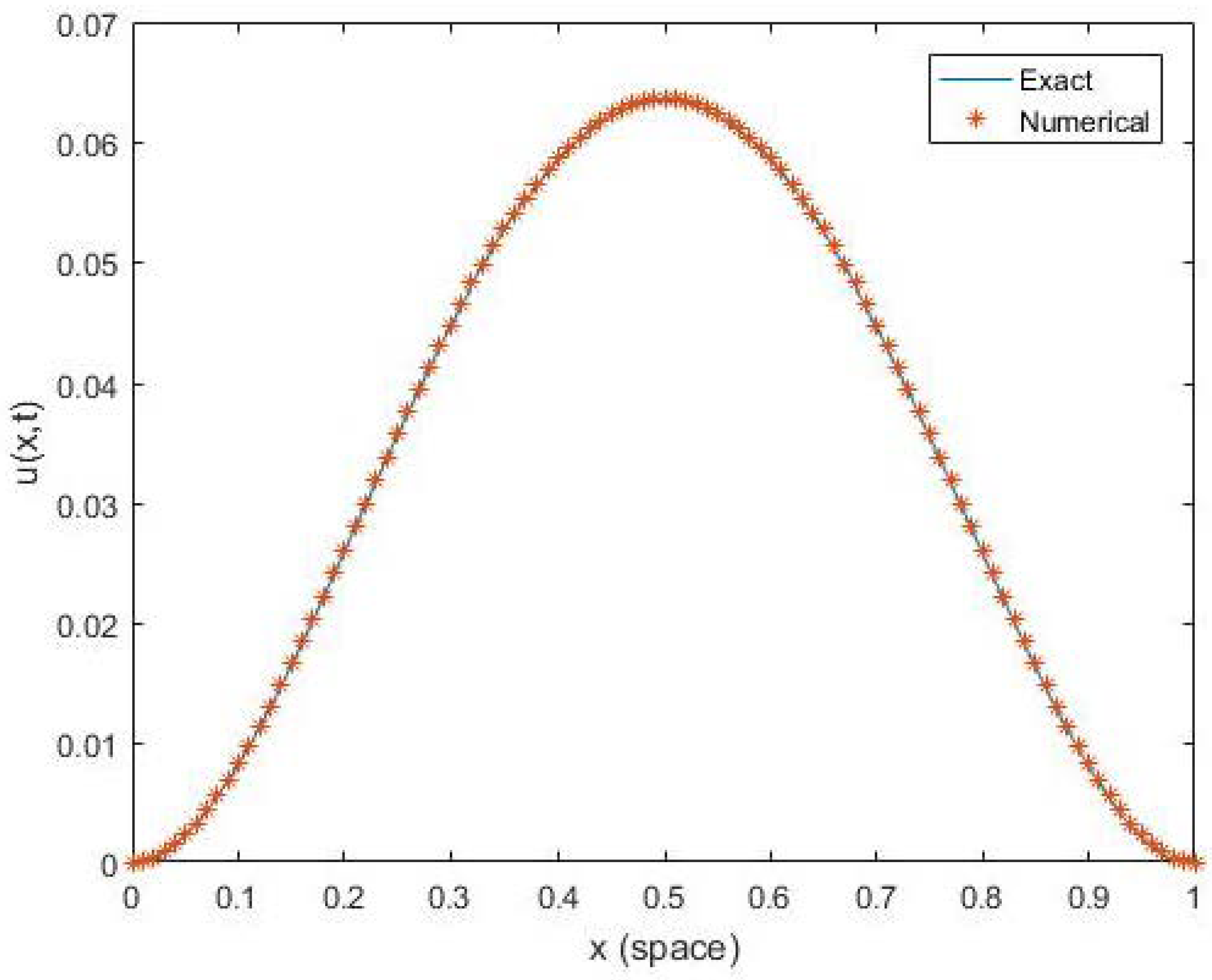
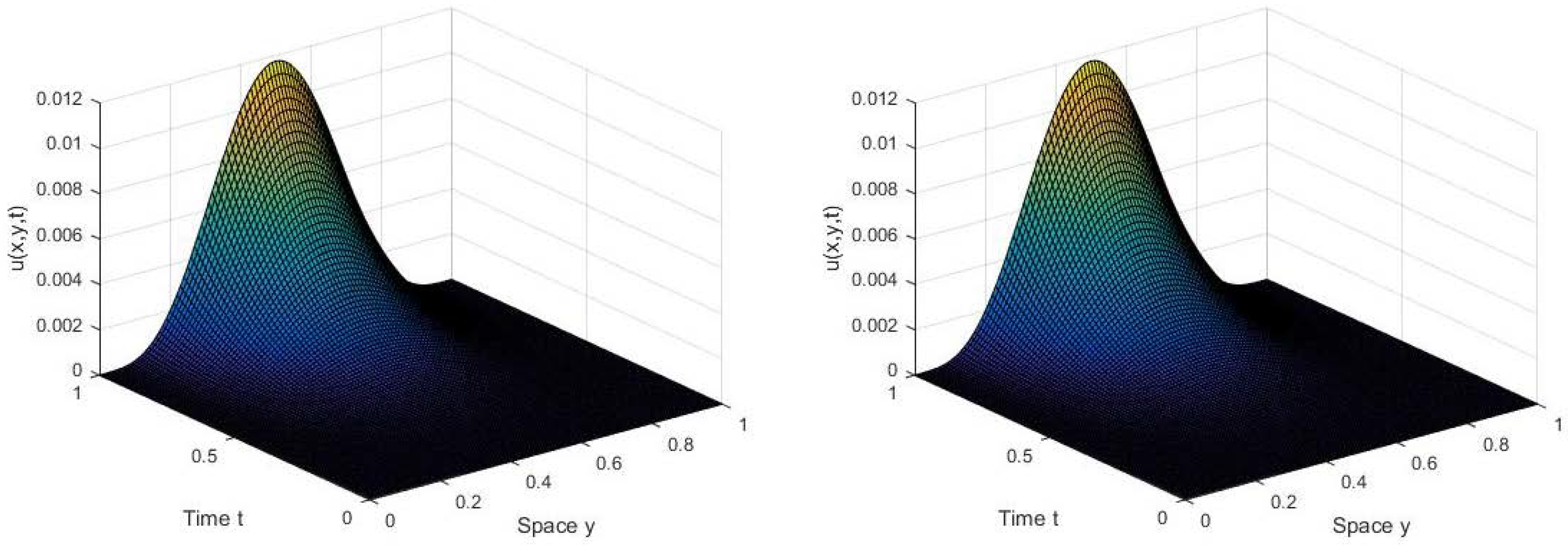
6. Numerical Simulations

1. Consider the one dimensional RSFCDEs over a bounded domain with initial and Dirichlet boundary conditions:

$$\left\{\begin{array}{c}{\displaystyle \frac{\partial u(x,y,t)}{\partial t}}=c_x{\displaystyle \frac{{\partial }^{\alpha }u(x,t}{{\partial \left|x\right|}^{\alpha }}}+d_x{\displaystyle \frac{{\partial }^{\beta }u(x,t}{{\partial \left|x\right|}^{\beta }}}+p(x,t),\hfill \\ u(x,0)=0,0<x\le 1,\hfill \\ u(0,t)=u(1,t)=0,0<t\le T,\hfill \end{array}\right.$$

with the source term:

$$\begin{array}{ccc}\hfill p(x,t)& =& t^{\beta -1}{e}^{\alpha t}(\beta +\alpha t)x^2{(1-x)}^2\hfill \\ & +& {\displaystyle \frac{c_x{t}^{\beta }{e}^{\alpha t}}{2cos(\alpha \pi /2}}[\frac{2}{\mathsf{\Gamma }(3-\alpha )}\left(x^{2-\alpha }+{(1-x)}^{2-\alpha }\right)\hfill \\ & -& \frac{12}{\mathsf{\Gamma }(4-\alpha }\left(x^{3-\alpha }+{(1-x)}^{3-\alpha }\right)+\frac{24}{\mathsf{\Gamma }(5-\alpha )}\left(x^{4-\alpha }+{(1-x)}^{4-\alpha }\right)]\hfill \\ & +& {\displaystyle \frac{d_x{t}^{\beta }{e}^{\alpha t}}{2cos(\beta \pi /2}}[\frac{2}{\mathsf{\Gamma }(3-\beta )}\left(x^{2-\beta }+{(1-x)}^{2-\beta }\right)\hfill \\ & -& \frac{12}{\mathsf{\Gamma }(4-\beta }\left(x^{3-\beta }+{(1-x)}^{3-\beta }\right)+\frac{24}{\mathsf{\Gamma }(5-\beta )}\left(x^{4-\beta }+{(1-x)}^{4-\beta }\right)].\hfill \end{array}$$

The exact solution is

$$u(x,t)=t^{\beta }{e}^{\alpha t}{x}^2{(1-x)}^2.$$

All the numerical simulations are done based on the finite space domain $\mathsf{\Omega }\times {\mathsf{\Omega }}_t$ where $\mathsf{\Omega }=[0,1]\times [0,1]$ and ${\mathsf{\Omega }}_t=[0,1]$. The order of convergence both in space and time are calculated using the formula:

$$\begin{array}{cc}\hfill Orde{r}_1& ={\displaystyle \frac{{\left|\right|E(h,\tau )\left|\right|}_{\infty }/{\left|\right|E(h/2,\tau /2)\left|\right|}_{\infty }}{log\left(2\right)}},\hfill \\ \hfill Orde{r}_2& ={\displaystyle \frac{\left|\right|E(h_x,h_y,\tau ){\left|\right|}_{\infty }/\left|\right|E(h_x/2,h_y/2,\tau /2){\left|\right|}_{\infty }}{log\left(2\right)}},\hfill \end{array}$$

(79)

where $orde{r}_1$ is the rate of convergence for one-dimensional two-sided space fractional convection–diffusion equation and $orde{r}_2$ is rate convergence of two dimensional two-sided space fractional equation. ${\left|\right|E(h,\tau )\left|\right|}_{\infty }$ is the maximum error for one dimensional space fractional problem and $\left|\right|E(h_x,h_y,\tau ){\left|\right|}_{\infty }$ for two dimensional space fractional problem, denoted as $Max-Error$. As we have seen in

Table 1. Convergence order and maximum error are produced with convection–dominance for example 1 at $T=1,c_x=2,d_x=0.25$.

		$\mathit{\alpha }=0.1$		$\mathit{\alpha }=0.45$		$\mathit{\alpha }=0.85$
	$\mathit{h}=\mathit{\tau }$	$\mathit{Max}-\mathit{Error}$	${\mathit{Order}}_{\mathbf{1}}$	$\mathit{Max}-\mathit{Error}$	${\mathit{Order}}_{\mathbf{1}}$	$\mathit{Max}-\mathit{Error}$	${\mathit{Order}}_{\mathbf{1}}$
	1/10	$8.3\times {10}^{-3}$	–	$1.21\times {10}^{-2}$	–	$1.70\times {10}^{-2}$	–
$\beta =1.25$	1/20	$2.2\times {10}^{-3}$	1.9156	$3.2\times {10}^{-3}$	1.9189	$4.4\times {10}^{-3}$	1.9500
	1/40	$5.5354\times {10}^{-4}$	1.9907	$8.0831\times {10}^{-4}$	1.9851	$1.1\times {10}^{-3}$	2.0000
	1/80	$1.3870\times {10}^{-4}$	2.0030	$2.0291\times {10}^{-4}$	1.9941	$2.7919\times {10}^{-4}$	1.9782
	1/160	$3.4320\times {10}^{-5}$	2.0086	$5.0701\times {10}^{-5}$	2.0008	$6.9932\times {10}^{-5}$	1.9972
	1/10	$8.8\times {10}^{-3}$	–	$1.24\times {10}^{-2}$	–	1.81$\times {10}^{-2}$	–
$\beta =1.85$	1/20	$2.4\times {10}^{-3}$	1.8745	$3.3\times {10}^{-3}$	1.9098	$4.8\times {10}^{-3}$	1.9149
	1/40	$6.0999\times {10}^{-4}$	1.9762	$8.5839\times {10}^{-4}$	1.9428	$1.2\times {10}^{-3}$	2.0000
	1/80	$1.5478\times {10}^{-4}$	1.9786	$2.1846\times {10}^{-4}$	1.9743	$3.1912\times {10}^{-4}$	1.9109
	1/160	$3.8968\times {10}^{-5}$	1.9899	$5.5120\times {10}^{-5}$	1.9867	$8.0991\times {10}^{-5}$	1.9783

, the second order convergence and the maximum error are confirmed at each grid size for convection-dominance (i.e., $c_x>d_x$) for one dimensional two-sided space fractional convection–diffusion equation with different space fractional order. As we have refined the grid size, the suitable maximum error is obtained. The convergence order and maximum error for a diffusion–dominance (i.e., $c_x<d_x)$ one dimensional two-sided space fractional convection–diffusion problem are shown in

Table 2. Convergence order and maximum error produced with diffusion-dominance for example 1 at $T=1,c_x=0.25,d_x=2$.

		$\mathit{\alpha }=0.1$		$\mathit{\alpha }=0.45$		$\mathit{\alpha }=0.85$
	$\mathit{h}=\mathit{\tau }$	$\mathit{Max}-\mathit{Error}$	${\mathit{Order}}_{\mathbf{1}}$	$\mathit{Max}-\mathit{Error}$	${\mathit{Order}}_{\mathbf{1}}$	$\mathit{Max}-\mathit{Error}$	${\mathit{Order}}_{\mathbf{1}}$
	1/10	$8.3\times {10}^{-3}$	–	$1.23\times {10}^{-2}$	–	$1.75\times {10}^{-2}$	–
$\beta =1.25$	1/20	$2.1\times {10}^{-3}$	1.9827	$3.2\times {10}^{-3}$	1.9425	$4.5\times {10}^{-3}$	1.9594
	1/40	$5.3416\times {10}^{-4}$	1.9750	$7.9693\times {10}^{-4}$	2.0055	$1.1\times {10}^{-3}$	2.0324
	1/80	$1.3389\times {10}^{-4}$	1.9962	$1.9979\times {10}^{-4}$	1.9960	$2.8337\times {10}^{-4}$	1.9567
	1/160	$3.3498\times {10}^{-5}$	1.9989	$4.9986\times {10}^{-5}$	1.9989	$7.0902\times {10}^{-5}$	1.9988
	1/10	$9.5\times {10}^{-3}$	–	$1.42\times {10}^{-2}$	–	$2.01\times {10}^{-2}$	–
$\beta =1.85$	1/20	$2.5\times {10}^{-3}$	1.9260	$3.7\times {10}^{-3}$	1.9403	$5.3\times {10}^{-3}$	1.9231
	1/40	$6.3804\times {10}^{-4}$	1.9702	$9.5140\times {10}^{-4}$	1.9594	$1.3\times {10}^{-3}$	2.0275
	1/80	$1.6126\times {10}^{-4}$	1.9843	$2.4052\times {10}^{-4}$	1.9839	$3.4116\times {10}^{-4}$	1.9300
	1/160	$4.0532\times {10}^{-5}$	1.9923	$6.0459\times {10}^{-5}$	1.9921	$8.5774\times {10}^{-5}$	1.9918

. Figure 1 shows the good agreement of exact and numerical solution of one-dimensional convection–diffusion equation with the coefficients $c_x=0.5,d_x=1.5$ and with fractional orders $\alpha =0.75,\beta =1.85$ at $N_x=N_t=100$ grid points.

2. Consider two-dimensional diffusion problem.($c_x=c_y=0$)

$$\left\{\begin{array}{c}{\displaystyle \frac{\partial u(x,y,t)}{\partial t}}=d_x{\displaystyle \frac{{\partial }^{{\beta }_1}u(x,y,t)}{{\partial \left|x\right|}^{{\beta }_2}}}+d_y{\displaystyle \frac{{\partial }^{{\beta }_2}u(x,y,t}{{\partial \left|y\right|}^{{\beta }_2}}}+p(x,y,t)\hfill \\ u(x,y,0)=x^2{(1-x)}^2{y}^2{(1-y)}^2,0<x\le 1,0<y\le 1,\hfill \\ {u(x,y,t)|}_{\partial \mathsf{\Omega }}=0,0<t\le T,1<{\beta }_1,{\beta }_2<2,\hfill \end{array}\right.$$

with the source term:

$$\begin{array}{ccc}\hfill p(x,y,t)& =& {\beta }_1{(t+1)}^{{\beta }_1-1}{x}^2{(1-x)}^2{\beta }_2{(t+1)}^{{\beta }_2-1}{y}^2{(1-y)}^2\hfill \\ & +& {\displaystyle \frac{d_x}{2cos({\beta }_1\pi /2}}{(t+1)}^{{\beta }_1}[\frac{2}{\mathsf{\Gamma }(3-{\beta }_1)}\left(x^{2-{\beta }_1}+{(1-x)}^{2-{\beta }_1}\right)\hfill \\ & -& \frac{12}{\mathsf{\Gamma }(4-{\beta }_1}\left(x^{3-{\beta }_1}+{(1-x)}^{3-{\beta }_1}\right)+\frac{24}{\mathsf{\Gamma }(5-{\beta }_1)}\left(x^{4-{\beta }_1}+{(1-x)}^{4-{\beta }_1}\right)]y^2{(1-y)}^2\hfill \\ & +& {\displaystyle \frac{d_y}{2cos({\beta }_2\pi /2}}{(t+1)}^{{\beta }_2}[\frac{2}{\mathsf{\Gamma }(3-{\beta }_2)}\left(y^{2-{\beta }_2}+{(1-y)}^{2-{\beta }_2}\right)\hfill \\ & -& \frac{12}{\mathsf{\Gamma }(4-{\beta }_2}\left(y^{3-{\beta }_2}+{(1-y)}^{3-{\beta }_2}\right)+\frac{24}{\mathsf{\Gamma }(5-{\beta }_2)}\left(y^{4-{\beta }_2}+{(1-y)}^{4-{\beta }_2}\right)]x^2{(1-x)}^2.\hfill \end{array}$$

(80)

Table 3. Convergence rate and maximum error produced for example 2 at $T=1,d_x=2=d_y,h_x=h_y=\tau$.

		${\mathit{\beta }}_1=1.25$		${\mathit{\beta }}_1=1.5$		${\mathit{\beta }}_1=1.95$
	${\mathit{h}}_{\mathit{x}},{\mathit{h}}_{\mathit{y}},\mathit{\tau }$	$\mathit{Max}-\mathit{Error}$	${\mathit{Order}}_{\mathbf{2}}$	$\mathit{Max}-\mathit{Error}$	${\mathit{Order}}_{\mathbf{2}}$	$\mathit{Max}-\mathit{Error}$	${\mathit{Order}}_{\mathbf{2}}$
	1/10	$2.57\times {10}^{-2}$	–	$2.75\times {10}^{-2}$	–	$1.56\times {10}^{-2}$	–
${\beta }_2=1.85$	1/20	$5.5\times {10}^{-3}$	2.2243	$6.3\times {10}^{-3}$	2.0283	$3.2\times {10}^{-3}$	2.2854
	1/40	$7.4176\times {10}^{-4}$	2.4894	$1.2\times {10}^{-3}$	2.3923	$7.9692\times {10}^{-4}$	2.0056
	1/80	$1.6630\times {10}^{-4}$	2.1565	$2.4526\times {10}^{-4}$	2.2907	$1.9977\times {10}^{-4}$	1.9961

shows that the maximum error and order of convergence for two-dimensional two-sided space fractional diffusion equation with different space fractional orders by taking $c_x=0=c_y$. For this numerical simulation, we have used same step-size for space and time (i.e., $h_x=h_y=\tau )$. The maximum time domain that used to obtain all the numerical results is $T=1$ and the diffusion coefficients are $d_x=2=d_y$. The surface plot of $u(x,y,t)$ with the diffusion coefficients $d_x=2.5$, $d_y=1.5,{\beta }_1=1.25,{\beta }_2=1.85$ at the mesh points $h_1=h_2=\tau =0.01$ is given in Figure 2.

3. Let us consider the two-dimensional Riesz space fractional convection–diffusion problem with bounded domain:

$$\left\{\begin{array}{c}{\displaystyle \frac{\partial u(x,y,t)}{\partial t}}=c_x{\displaystyle \frac{{\partial }^{{\alpha }_1}u(x,y,t}{{\partial \left|x\right|}^{{\alpha }_1}}}+c_y{\displaystyle \frac{{\partial }^{{\alpha }_2}u(x,y,t}{{\partial \left|y\right|}^{{\alpha }_2}}}+d_x{\displaystyle \frac{{\partial }^{{\beta }_1}u(x,y,t}{{\partial \left|x\right|}^{{\beta }_1}}}+d_y{\displaystyle \frac{{\partial }^{{\beta }_2}u(x,y,t}{{\partial \left|y\right|}^{{\beta }_2}}}+p(x,y,t)\hfill \\ u(x,y,0)=0,0<x\le 1,0<y\le 1,\hfill \\ {u(x,y,t)|}_{\partial \mathsf{\Omega }}=0,0\le t\le T,\hfill \end{array}\right.$$

with the source term:

$$\begin{array}{ccc}\hfill p(x,y,t)& =& t^{{\beta }_1-1}{e}^{{\alpha }_{1}t}({\beta }_1+{\alpha }_{1}t)x^2{(1-x)}^2{y}^2{(1-y)}^2\hfill \\ & +& {\displaystyle \frac{c_x{t}^{{\beta }_1}{e}^{{\alpha }_{1}t}}{2cos({\alpha }_1\pi /2)}}[\frac{2}{\mathsf{\Gamma }(2-{\alpha }_1)}\left(x^{2-{\alpha }_1}+{(1-x)}^{2-{\alpha }_1}\right)\hfill \\ & -& \frac{12}{\mathsf{\Gamma }(4-{\alpha }_1}\left(x^{3-{\alpha }_1}+{(1-x)}^{3-{\alpha }_1}\right)+\frac{24}{\mathsf{\Gamma }(5-{\alpha }_1)}\left(x^{4-{\alpha }_1}+{(1-x)}^{4-{\alpha }_1}\right)]y^2{(1-y)}^2\hfill \\ & +& {\displaystyle \frac{c_y{t}^{{\beta }_2}{e}^{{\alpha }_{2}t}}{2cos({\alpha }_2\pi /2)}}[\frac{2}{\mathsf{\Gamma }(2-{\alpha }_2)}\left(y^{2-{\alpha }_2}+{(1-y)}^{2-{\alpha }_2}\right)\hfill \\ & -& \frac{12}{\mathsf{\Gamma }(4-{\alpha }_2}\left(y^{3-{\alpha }_2}+{(1-y)}^{3-{\alpha }_2}\right)+\frac{24}{\mathsf{\Gamma }(5-{\alpha }_2)}\left(y^{4-{\alpha }_2}+{(1-y)}^{4-{\alpha }_2}\right)]x^2{(1-x)}^2\hfill \\ & +& {\displaystyle \frac{d_x{t}^{{\beta }_1}{e}^{{\alpha }_{1}t}}{2cos({\beta }_1\pi /2)}}[\frac{2}{\mathsf{\Gamma }(2-{\beta }_1)}\left(x^{2-{\beta }_1}+{(1-x)}^{2-{\beta }_1}\right)\hfill \\ & -& \frac{12}{\mathsf{\Gamma }(4-{\beta }_1}\left(x^{3-{\beta }_1}+{(1-x)}^{3-{\beta }_1}\right)+\frac{24}{\mathsf{\Gamma }(5-{\beta }_1)}\left(x^{4-{\beta }_1}+{(1-x)}^{4-{\beta }_1}\right)]y^2{(1-y)}^2\hfill \\ & +& {\displaystyle \frac{d_y{t}^{{\beta }_2}{e}^{{\alpha }_{2}t}}{2cos({\beta }_2\pi /2)}}[\frac{2}{\mathsf{\Gamma }(2-{\beta }_2)}\left(y^{2-{\beta }_2}+{(1-y)}^{2-{\beta }_2}\right)\hfill \\ & -& \frac{12}{\mathsf{\Gamma }(4-{\beta }_2}\left(y^{3-{\beta }_1}+{(1-y)}^{3-{\beta }_2}\right)+\frac{24}{\mathsf{\Gamma }(5-{\beta }_2)}\left(y^{4-{\beta }_2}+{(1-y)}^{4-{\beta }_2}\right)]x^2{(1-x)}^2\hfill \end{array}$$

The exact solution is,

$$u(x,y,t)=t^{\beta }{e}^{\alpha t}{x}^2{(1-x)}^2{y}^2{(1-y)}^2.$$

In

Table 4. Convergence order produced with diffusion-dominance for example 3 at $T=1,c_x=0.25=c_y,d_x=2=d_y,h_x=h_y=\tau$.

		${\mathit{\alpha }}_1=0.5$		${\mathit{\alpha }}_1=0.75$		${\mathit{\alpha }}_1=0.95$
	${\mathit{h}}_{\mathit{x}},{\mathit{h}}_{\mathit{y}},\mathit{\tau }$	$\mathit{Max}-\mathit{Error}$	${\mathit{Order}}_{\mathbf{2}}$	$\mathit{Max}-\mathit{Error}$	${\mathit{Order}}_{\mathbf{2}}$	$\mathit{Max}-\mathit{Error}$	${\mathit{Order}}_{\mathbf{2}}$
	1/10	$2.00\times {10}^{-2}$	–	$2.09\times {10}^{-2}$	–	$2.6\times {10}^{-3}$	–
${\beta }_1=1.25$	1/20	5.7$\times {10}^{-3}$	1.8110	$6.1\times {10}^{-3}$	1.7766	$6.4607\times {10}^{-4}$	2.0087
	1/40	$1.7\times {10}^{-3}$	1.7454	$1.9\times {10}^{-3}$	1.6828	$1.4898\times {10}^{-4}$	2.1166
	1/80	$2.8802\times {10}^{-4}$	1.9962	$6.6947\times {10}^{-4}$	1.7467	$2.9810\times {10}^{-5}$	2.3213
	1/10	$1.52\times {10}^{-2}$	–	$2.06\times {10}^{-2}$	–	$2.34\times {10}^{-2}$	–
${\beta }_1=1.85$	1/20	$3.6\times {10}^{-3}$	2.0780	$5.00\times {10}^{-3}$	2.0426	$5.5\times {10}^{-3}$	2.0890
	1/40	$7.6214\times {10}^{-4}$	2.2399	1.1$\times {10}^{-3}$	2.1844	$1.0001\times {10}^{-3}$	2.4595
	1/80	$1.0496\times {10}^{-4}$	2.4602	$1.7907\times {10}^{-4}$	2.6189	$1.8006\times {10}^{-4}$	2.4735
	1/160	$1.9729\times {10}^{-5}$	2.4114	$2.7175\times {10}^{-5}$	2.5202	$3.5515\times {10}^{-5}$	2.3420

, we have found a numerical results that produce second order convergence rate and maximum error for two sided two dimensional space fractional convection–diffusion equation with diffusion–dominance ($c_x=0.25=c_y,d_x=d_y=2$) phenomena. For this simulation we have taken a fixed value for ${\beta }_2({\beta }_2=1.75)$ and for ${\alpha }_2({\alpha }_2=0.5)$ with different values for ${\alpha }_1,{\beta }_1$. Similarly in

Table 5. Convergence order produced with convection-dominance for example 3 at $T=1,c_x=2=c_y,d_x=0.25=d_y,h_x=h_y=\tau$.

		${\mathit{\alpha }}_1=0.5$		${\mathit{\alpha }}_1=0.75$		${\mathit{\alpha }}_1=0.95$
	${\mathit{h}}_{\mathit{x}},{\mathit{h}}_{\mathit{y}},\mathit{\tau }$	$\mathit{Max}-\mathit{Error}$	${\mathit{Order}}_{\mathbf{2}}$	$\mathit{Max}-\mathit{Error}$	${\mathit{Order}}_{\mathbf{2}}$	$\mathit{Max}-\mathit{Error}$	${\mathit{Order}}_{\mathbf{2}}$
	1/10	$1.51\times {10}^{-2}$	–	$1.09\times {10}^{-2}$	–	$4.1\times {10}^{-3}$	–
${\beta }_1=1.25$	1/20	2.00$\times {10}^{-3}$	2.3163	1.9$\times {10}^{-3}$	2.5203	$1.4\times {10}^{-3}$	1.6502
	1/40	$5.8273\times {10}^{-4}$	1.7791	4.8275$\times {10}^{-4}$	1.9767	$2.7307\times {10}^{-4}$	2.3581
	1/80	$1.8883\times {10}^{-4}$	1.6257	$1.5338\times {10}^{-4}$	1.6542	$5.5304\times {10}^{-5}$	2.3038
	1/10	$1.80\times {10}^{-2}$	–	$1.75\times {10}^{-2}$	–	$1.39\times {10}^{-2}$	–
${\beta }_1=1.85$	1/20	$4.3\times {10}^{-3}$	2.0656	$4.1\times {10}^{-3}$	2.0937	$2.4\times {10}^{-3}$	2.5340
	1/40	$8.7170\times {10}^{-4}$	2.3024	$7.6626\times {10}^{-4}$	2.4197	$5.5154\times {10}^{-4}$	2.1215
	1/80	$1.7428\times {10}^{-4}$	2.3224	$1.3016\times {10}^{-4}$	2.5575	$1.29899\times {10}^{-4}$	2.0861

, we have considered the convection–dominance ($c_x=2=c_y,d_x=d_y=0.25$) two-sided two-dimensional space fractional convection–diffusion problem with fixed ${\beta }_2({\beta }_2=1.75)$ and for fixed ${\alpha }_2({\alpha }_2=0.5)$. The order of convergence and maximum errors are calculated using the formula expressed in Equation (79). In Figure 3 the surface plot of exact and numerical solutions for two-dimensional convection–diffusion equations are investigated by considering the coefficients $c_x=c_y=2.5,d_x=d_y=1.5$ with orders ${\alpha }_1=0.75,{\alpha }_2=0.75,{\beta }_1=1.85,{\beta }_2=1.85$ at $N_x=N_y=N_t=100$ mesh grid points.

7. Conclusions

In our study, we have developed an algorithm for two-dimensional two-sided space fractional convection–diffusion problem using the CNADI difference method for time discretization combined with WSGD scheme for the approximation of space fractional derivative. We have used a shifted category of standard Grünwald-Letnikov difference method and weighted version of the shifted Grünwald-Letnikov difference approximation with CNADI scheme to have unconditionally stable and second order convergence both in space and time without extrapolation. Moreover, unconditional stability and second order convergence is justified for convection-dominance two-sided two dimension space fractional convection–diffusion equation. Our theoretical study and analysis has been confirmed by our numerical simulation in Section 6. We will consider the space fractional reaction convection–diffusion equation in our near further research.

References

1. Podlubny, I. Fractional Differential Equations: An Introduction to Fractional Derivatives, Fractional Differential Equations, to Methods of Their Solution and Some of Their Applications; Elsevier: New York, NY, USA, 1998; Volume 198. [Google Scholar]
2. Li, C.; Zeng, F. Finite difference methods for fractional differential equations. Int. J. Bifurcat. Chaos 2012, 22, 1230014. [Google Scholar] [CrossRef]
3. Diethelm, K. The Analysis of Fractional Differential Equations; Springer Science & Business Media: Berlin/Heidelberg, Germany, 2010. [Google Scholar]
4. Fomin, S.; Chugunov, V.; Hashida, T. Application of fractional differential equations for modeling the anomalous diffusion of contaminant from fracture into porous rock matrix with bordering alteration zone. Trans. Porous Med. 2010, 81, 187–205. [Google Scholar] [CrossRef]
5. Salman, W.; Gavriilidis, A.; Angeli, P. A model for predicting axial mixing during gas–liquid Taylor flow in microchannels at low Bodenstein number. Chem. Eng. J. 2004, 101, 391–396. [Google Scholar] [CrossRef]
6. Berkowitz, B.; Cortis, A.; Dror, I.; Scher, H. Laboratory experiments on dispersive transport across interfaces. Water Resour. Res. 2009, 45. [Google Scholar] [CrossRef] [Green Version]
7. Cortis, A.; Berkowitz, B. Computing “anomalous” contaminant transport in porous media. Ground Water 2005, 43, 947–950. [Google Scholar] [CrossRef]
8. Wang, K.; Wang, H. A fast characteristic finite difference method for fractional advection–diffusion equations. Adv. Water. Resour. 2011, 34, 810–816. [Google Scholar] [CrossRef]
9. Singh, J.; Swroop, R.; Kumar, D. A computational approach for fractional convection–diffusion equation via integral transforms. Ain Shams Eng. J. 2016, 9, 1019–1028. [Google Scholar] [CrossRef] [Green Version]
10. Wang, Y.M. A compact finite difference method for a class of time fractional convection–diffusion-wave equations with variable coefficients. Numer. Algorithms 2015, 70, 625–651. [Google Scholar] [CrossRef]
11. Gu, X.M.; Huang, T.Z.; Ji, C.C.; Carpentieri, B.; Alikhanov, A.A. Fast iterative method with a second-order implicit difference scheme for time-space fractional convection–diffusion equation. J. Sci. Comput. 2017, 72, 957–985. [Google Scholar] [CrossRef]
12. Cui, M. Combined compact difference scheme for the time fractional convection–diffusion equation with variable coefficients. Appl. Math. Comput. 2014, 246, 464–473. [Google Scholar] [CrossRef]
13. Tian, W.; Deng, W.; Wu, Y. Polynomial spectral collocation method for space fractional advection–diffusion equation. Numer. Methods Partial Differ. Equ. 2014, 30, 514–535. [Google Scholar] [CrossRef] [Green Version]
14. Bhrawy, A.H.; Baleanu, D. A spectral Legendre–Gauss–Lobatto collocation method for a space-fractional advection–diffusion equations with variable coefficients. Rep. Math. Phys. 2013, 72, 219–233. [Google Scholar] [CrossRef]
15. Saadatmandi, A.; Dehghan, M.; Azizi, M.R. The Sinc-Legendre collocation method for a class of fractional convection–diffusion equations with variable coefficients. Commun. Nonlinear Sci. Numer. Simul. 2012, 17, 4125–4136. [Google Scholar] [CrossRef]
16. Parvizi, M.; Eslahchi, M.R.; Dehghan, M. Numerical solution of fractional advection-diffusion equation with a nonlinear source term. Numer. Algorithms 2015, 68, 601–629. [Google Scholar] [CrossRef]
17. Li, C.; Zeng, F. Numerical Methods for Fractional Calculus; Chapman and Hall/CRC: Boca Raton, FL, USA, 2015. [Google Scholar]
18. Jin, B.; Lazarov, R.; Zhou, Z. A Petrov–Galerkin finite element method for fractional convection–diffusion equations. SIAM J. Numer. Anal. 2016, 54, 481–503. [Google Scholar] [CrossRef] [Green Version]
19. Aboelenen, T. A direct discontinuous Galerkin method for fractional convection–diffusion and Schrödinger-type equations. Eur. Phys. J. Plus 2018, 133, 316. [Google Scholar] [CrossRef]
20. Xu, Q.; Hesthaven, J.S. Discontinuous Galerkin method for fractional convection–diffusion equations. SIAM J. Numer. Anal. 2014, 52, 405–423. [Google Scholar] [CrossRef] [Green Version]
21. Gao, F.; Yuan, Y.; Du, N. An upwind finite volume element method for nonlinear convection–diffusion problem. AJCM 2011, 1, 264. [Google Scholar] [CrossRef] [Green Version]
22. Badr, M.; Yazdani, A.; Jafari, H. Stability of a finite volume element method for the time-fractional advection-diffusion equation. Numer. Methods Partial Differ. Equ. 2018, 34, 1459–1471. [Google Scholar] [CrossRef]
23. Ding, H.F.; Zhang, Y.X. New numerical methods for the Riesz space fractional partial differential equations. Comput. Math. Appl. 2012, 63, 1135–1146. [Google Scholar]
24. Anley, E.F.; Zheng, Z. Finite Difference Approximation Method for a Space Fractional Convection–Diffusion Equation with Variable Coefficients. Symmetry 2020, 12, 485. [Google Scholar] [CrossRef] [Green Version]
25. Zhang, Y.N.; Sun, Z.Z. Alternating direction implicit schemes for the two-dimensional fractional sub-diffusion equation. J. Comput. Phys. 2011, 230, 8713–8728. [Google Scholar] [CrossRef]
26. Tadjeran, C.; Meerschaert, M.M. A second-order accurate numerical method for the two-dimensional fractional diffusion equation. J. Comput. Phys. 2007, 220, 813–823. [Google Scholar] [CrossRef]
27. Meerschaert, M.M.; Scheffler, H.P.; Tadjeran, C. Finite difference methods for two-dimensional fractional dispersion equation. J. Comput. Phys. 2006, 211, 249–261. [Google Scholar] [CrossRef]
28. Valizadeh, S.; Borhanifar, A.; Malek, A. Compact ADI method for solving two-dimensional Riesz space fractional diffusion equation. arXiv 2018, arXiv:1802.02015. [Google Scholar]
29. Wang, H.; Basu, T.S. A fast finite difference method for two-dimensional space-fractional diffusion equations. SIAM J. Sci. Comput. 2012, 34, A2444–A2458. [Google Scholar] [CrossRef]
30. Yin, X.; Fang, S.; Guo, C. Alternating-direction implicit finite difference methods for a new two-dimensional two-sided space-fractional diffusion equation. Adv. Diff. Equ. 2018, 2018, 389. [Google Scholar] [CrossRef]
31. Bu, W.; Tang, Y.; Yang, J. Galerkin finite element method for two-dimensional Riesz space fractional diffusion equations. J. Comput. Phys. 2014, 276, 26–38. [Google Scholar] [CrossRef]
32. Li, J.; Liu, F.; Feng, L.; Turner, I. A novel finite volume method for the Riesz space distributed-order diffusion equation. Comput. Appl. 2017, 74, 772–783. [Google Scholar] [CrossRef]
33. Chen, H.; Lv, W.; Zhang, T. A Kronecker product splitting preconditioner for two-dimensional space-fractional diffusion equations. J. Comput. Phys. 2018, 360, 1–14. [Google Scholar] [CrossRef]
34. Liu, F.; Chen, S.; Turner, I.; Burrage, K.; Anh, V. Numerical simulation for two-dimensional Riesz space fractional diffusion equations with a nonlinear reaction term. Cent. Eur. J. Phys. 2013, 11, 1221–1232. [Google Scholar] [CrossRef] [Green Version]
35. Zeng, F.; Liu, F.; Li, C.; Burrage, K.; Turner, I.; Anh, V. A Crank–Nicolson ADI spectral method for a two-dimensional Riesz space fractional nonlinear reaction-diffusion equation. SIAM J. Numer. Anal. 2014, 52, 2599–2622. [Google Scholar] [CrossRef] [Green Version]
36. Balasim, A.T.; Ali, N.H.M. New group iterative schemes in the numerical solution of the two-dimensional time fractional advection-diffusion equation. Cogent Math. 2017, 4, 1412241. [Google Scholar] [CrossRef]
37. Zhao, Y.; Bu, W.; Huang, J.; Liu, D.Y.; Tang, Y. Finite element method for two-dimensional space-fractional advection–dispersion equations. Appl. Math. Comput. 2015, 257, 553–565. [Google Scholar] [CrossRef]
38. Pang, G.; Chen, W.; Sze, K.Y. A comparative study of finite element and finite difference methods for two-dimensional space-fractional advection–dispersion equation. Adv. Appl. Math. Mech. 2016, 8, 166–186. [Google Scholar] [CrossRef]
39. Li, J.; Liu, F.; Feng, L.; Turner, I. A novel finite volume method for the Riesz space distributed-order advection–diffusion equation. Appl. Math. Model. 2017, 46, 536–553. [Google Scholar] [CrossRef] [Green Version]
40. Chen, M.; Deng, W. A second-order numerical method for two-dimensional two-sided space fractional convection- diffusion equation. Appl. Math. Model. 2014, 38, 3244–3259. [Google Scholar] [CrossRef]
41. Zhang, Y.N.; Sun, Z.Z.; Zhao, X. Compact alternating direction implicit scheme for the two-dimensional fractional diffusion-wave equation. SIAM J. Numer. Anal. 2012, 50, 1535–1555. [Google Scholar] [CrossRef]
42. Benson, D.A.; Wheatcraft, S.; Meerschaert, M.M. Application of a fractional advection–dispersion equation. Water Resour. Res. 2000, 36, 1403–1412. [Google Scholar] [CrossRef] [Green Version]
43. Zhang, Y.; Meerschaert, M.M.; Neupauer, R.M. Backward fractional advection dispersion model for contaminant source prediction. Water Resour. Res. 2016, 52, 2462–2473. [Google Scholar] [CrossRef] [Green Version]
44. Samko, S.G.; Kilbas, A.A.; Marichev, O.I. Fractional Integrals and Derivatives; Gordon and Breach Science Publisher: Yverdon, Switzerland, 1993; Volume 1. [Google Scholar]
45. Podlubny, I. Fractional Differential Equations Academic; Academic Press: New York, NY, USA, 1999. [Google Scholar]
46. Tian, W.; Zhou, H.; Deng, W. A class of second order difference approximations for solving space fractional diffusion equations. Math. Comp. 2015, 84, 1703–1727. [Google Scholar] [CrossRef] [Green Version]
47. Liu, F.; Zhuang, P.; Anh, V.; Turner, I.; Burrage, K. Stability and convergence of the difference methods for the space–time fractional advection–diffusion equation. Appl. Math. Comput. 2007, 191, 12–20. [Google Scholar] [CrossRef]
48. Feng, L.; Zhuang, P.; Liu, F.; Turner, I.; Li, J. High-order numerical methods for the Riesz space fractional advection-dispersion equations. arXiv 2020, arXiv:2003.13923. [Google Scholar] [CrossRef]
49. Yang, Q.; Liu, F.; Turner, I. Numerical methods for fractional partial differential equations with Riesz space fractional derivatives. Appl. Math. Model. 2010, 34, 200–218. [Google Scholar] [CrossRef] [Green Version]
50. Shen, S.; Liu, F.; Anh, V.; Turner, I. The fundamental solution and numerical solution of the Riesz fractional advection–dispersion equation. IMA J. Appl. Math. 2008, 73, 850–872. [Google Scholar] [CrossRef]
51. Laub, A.J. Matrix Analysis for Scientists and Engineers; SIAM: Philadelphia, PA, USA, 2005; Volume 91. [Google Scholar]
52. Isaacson, E.; Keller, H.B. Analysis of Numerical Methods; Courier Corporation: Chelmsford, MA, USA, 2012. [Google Scholar]
Figure 1. Comparison of exact and numerical solution for one-dimensional convection–diffusion equations (CDEs) at α = 0.75 , β = 1.85 for numerical example 1.
Mathematics 08 01878 g001
Figure 2. Surface of u ( x , y , t ) for two-dimensional diffusion equation with m a x e r r o r = 1.7563 × 10 4 , β 1 = 1.25 , β 2 = 1.85 for numerical example 2.
Mathematics 08 01878 g002
Figure 3. The surface of u(x,y,t) for α 1 = 0.75 , α 2 = 0.75 , β 1 = 1.85 , β 2 = 1.85 for numerical example 3.
Mathematics 08 01878 g003