High Dimensional Hyperbolic Geometry of Complex Networks

Abstract

High dimensional embeddings of graph data into hyperbolic space have recently been shown to have great value in encoding hierarchical structures, especially in the area of natural language processing, named entity recognition, and machine generation of ontologies. Given the striking success of these approaches, we extend the famous hyperbolic geometric random graph models of Krioukov et al. to arbitrary dimension, providing a detailed analysis of the degree distribution behavior of the model in an expanded portion of the parameter space, considering several regimes which have yet to be considered. Our analysis includes a study of the asymptotic correlations of degree in the network, revealing a non-trivial dependence on the dimension and power law exponent. These results pave the way to using hyperbolic geometric random graph models in high dimensional contexts, which may provide a new window into the internal states of network nodes, manifested only by their external interconnectivity.

1. Introduction

Many complex networks, which arise from extremely diverse areas of study, surprisingly share a number of common properties. They are sparse, in the sense that the number of edges scales only linearly with the number of nodes, they have small radius, connected nodes tend to have many of their neighbors in common (beyond what would be expected from, for example, random graphs drawn from a distribution with a fixed degree sequence), and their degree sequence has a power law tail, generally with an exponent less than 3 [1,2,3,4]. One of the major efforts of network science is to devise models which are able to simultaneously capture these common properties.

Many models of complex networks have been proposed which are able to capture some of the common properties above. Perhaps the most well known is the Barabási–Albert model of preferential attachment [5]. This model is described in terms of a growing network, in which nodes of high degree are more likely to attract connections from newly born nodes. It is effective in capturing the power law degree sequence, but fails to generate graphs in which connected nodes tend to have a large fraction of their neighbors in common (often called ‘strong clustering’). There are growing indications that the strong clustering, the tendency for affiliation of neighbors of connected nodes, is a manifestation of the network having a geometric structure [6], based upon the notion of a geometric random graph. However, geometric random graphs based upon a flat, Euclidean geometry do not give rise to power law degree distributions. Curved space, on the other hand, in particular the negatively curved space of hyperbolic geometry, does give rise to such heterogeneous distribution of degrees, as shown by Krioukov et al. [7]. Random geometric graphs in hyperbolic geometry therefore provide extremely promising models for the structure of complex networks. Besides curvature, an arguably even more fundamental aspect of a geometric space is its dimension. After all, a lot more possibilities open when one is attempting to navigate a space of higher dimension. Can random geometric graph models based on higher dimensional geometry account for structures in graphs which so far have eluded description within lower dimensional models?

Recent developments in machine learning for natural language processing suggest that this is likely the case, as higher dimensional hyperbolic geometries prove more effective at link prediction in author collaboration networks than do embeddings into lower dimensional hyperbolic space [8]. High dimensional hyperbolic embeddings are also proving fruitful in representing taxonomic information within machine generated knowledge bases [9,10]. It may be worth noting that, in these machine learning contexts, the hyperbolic geometry generally plays a slightly different role. There one often seeks an isometric embedding of some structured data, such as word proximity graphs in natural language texts, into hyperbolic space of some dimension. In our approach based upon random geometric graphs, we are taking the geometric description more fundamentally, as we seek an embedding which covers the entire space uniformly, rather than covering merely an isometric subset of the space. The idea, ultimately, is to associate data with a dynamical description of geometry, for example, as is done in gravitational physics [11].

We consider statistical mechanical models of complex networks as introduced in [12], and, in particular, their application to random geometric graphs in hyperbolic space [7]. Fountoulakis has computed the asymptotic distribution of the degree of an arbitrary vertex in the hyperbolic model, and shown that it gives rise to a degree sequence which follows a power law [13]. More generally, it is known that the hyperbolic models are effective in capturing all of the above properties, including the strong clustering behavior which typically evades non-geometric models. Fountoulakis also proves that the degrees of any finite collection of vertices are asymptotically independent, so that in this sense the correlations that one might expect from spatial proximity vanish in the $N\to \infty$ and $R\to \infty$ limit. Furthermore, it is possible to assign an effective meaning to the dimensions of the hyperbolic embedding space: the radial dimension can be regarded as a measure of popularity of a network node, while the angular dimension acts as a space in which the similarity of nodes can be represented, such that nearby nodes are similar to each other, while distant nodes are not [14].

As far as we are aware, to date, all attention on this model has been focused on two -dimensional hyperbolic space. Generalization to higher dimension does appear in an as yet unpublished manuscript [15], which extends the hyperbolic geometric models to arbitrary dimension, however, explicit proofs regarding the degree distribution are not provided. High dimensional hyperbolic embeddings have also been explored from the machine learning perspective, but not as an explicit model of random geometric graphs as considered here [8]. It is reasonable to expect that, in order to capture the behavior of real world complex networks, it will be necessary to allow for similarity spaces of larger than one dimension. We therefore construct a model of random geometric graphs in a ball of ${\mathbb{H}}^{d+1}$, in direct analogy to the $d=1$ construction of [7]. In this model, the radial coordinate retains its effective meaning as a measure of the popularity of a node, while the similarity space becomes a full d-sphere, allowing for a much richer characterization of the interests of a person in a social network, or the role of an entity in some complex organizational structure. We perform a careful asymptotic analysis, yielding precise results which help clarify various aspects of the model.

In particular, we compute the asymptotic degree distribution in five regions of the parameter space, for arbitrary dimension, only one region of which ($\tau <1$ and $2\sigma >1$) was considered in Fountoulakis’ treatment of $d=1$ [13]. For $d=1$, the angular probability distribution is simply a constant $\frac{1}{2\pi }$, while when $d>1$ it is a dimension-dependent power of the sine of the angular separation between two nodes, so that we cannot expect to straightforwardly generalize the prior results for $d=1$ to higher dimension. In fact, the angular integrals are tedious and not easy to compute. We use the series expansion to decompose the integrated function, to get a fine infinitesimal estimation of the angular integral, which is the key step to performing the high dimensional analysis.

For $d=1$ Fountoulakis also computes the correlation of node degrees in the model, and shows that it goes to zero in the asymptotic limit [13]. We generalize this result to arbitrary dimension, finding that the asymptotic independence of degree requires a steeper fall off for the degree distribution (governed by the parameter $\sigma$) at larger dimension d. This dimensional dependence is reasonable, in the sense that, in higher dimensions, there are more directions in which nodes can interact. When computing clustering for the high dimensional model, the non-trivial angular dependence will pose an even greater challenge, since for three nodes there is much less angular symmetry. Hence our present analysis paves the way for future research in high dimensional hyperbolic space.

Our model employs a random mapping of graph nodes to points in a hyperbolic ball, giving these nodes hyperbolic coordinates, and connecting pairs of nodes if they are nearby in the hyperbolic geometry. Based upon their close relationship with hyperbolic geometry, we might assume that they are therefore intrinsically hyperbolic, in the sense of Gromov’s notion of $\delta$-hyperbolicity. This may be an important question, in that it would connect to a number of important results on hyperbolicity of graphs [16], and may cast an important light on the relevance of these hyperbolic geometric models to real world networks [17]. We do not expect our model to generate $\delta$-hyperbolic networks for the entire range of the parameter space of our model because, for example, one can effectively send the curvature to zero by choosing $R\ll 1$ (with $\zeta \equiv 1$). However, we would expect it to be the case when the effect of curvature is large, such as when R grows rapidly with respect to N. We do not know for certain whether the particular ranges of parameters that we explore in this paper generate $\delta$-hyperbolic graphs for $\delta >0$, almost surely, but imagine it likely to be the case.

1.1. Model Introduction

We consider a class of exponential random graph models, which are Gibbs (or Boltzmann) distributions on random labeled graphs. [12,18] These models define a probability distribution on graphs which is defined in terms of a Hamiltonian ‘energy functional’, for which the probability of a graph G is $Pr(G)=\frac{e^{-H(G)/T}}{Z(T)}$. T is a ‘temperature’, which controls the relevance of the Hamiltonian $H(G)$, and $Z(T)={\sum }_G{e}^{-H(G)/T}$ is a normalizing factor, often called the ‘partition function’. Note that the probability distribution becomes uniform in the limit $T\to \infty$. The Hamiltonian, which encodes the ‘energy’ of the graph, consists of a sum of ‘observables’, each multiplied by a corresponding Lagrange multiplier, which controls the relevance of that observables’ value in the probability of a given graph. We begin with the most general model for which the probability of each edge is independent, wherein each probability is governed by its own Lagrange multiplier ${\omega }_{u,v}$. Thus, our Hamiltonian is $H(G)={\sum }_{u<v}{\omega }_{u,v}{a}_{u,v}$, where $a_{u,v}=1$ if u and v are connected by an edge in G, and 0 otherwise. The partition function $Z(T)={\prod }_{u<v}(1+e^{-{\omega }_{u,v}/T})$, and the therefore the probability of occurrence of an edge between vertices u and v is

$$p_{u,v}=\frac{1}{1+e^{{\omega }_{u,v}/T}}.$$

Following [7], we embed each of N nodes into a hyperbolic ball of finite radius R in ${\mathbb{H}}^{d+1}$, and set the ‘link energies’ ${\omega }_{u,v}$ to be based on the distances $d_{u,v}$ between the embedded locations of the vertices u and v, through here we allow all integer values of $d\ge 1$. In particular, we set

$${\omega }_{u,v}=d_{u,v}-\mu ,$$

(1)

where $\mu$ is a connectivity distance threshold. Note that each pair of vertices for which $d_{u,v}<\mu$ contribute negatively to the ‘total energy’ whenever a link between them is present, so that the ‘ground state’ (minimum energy, highest probability) graph will have links between every pair of vertices $u,v$ for which $d_{u,v}<\mu$, and no links with $d_{u,v}>\mu$. Note that in the limit as $T\to 0$, the probability of the ground state graph goes to 1, and that of every other graph vanishes. Thus

$$p_{u,v}=\frac{1}{1+e^{\frac{d_{u,v}-\mu }{T}}}.$$

In a real world network, we may expect the largest node degree to be comparable with N itself, and the lowest degree nodes to have degree of order 1. To maintain this behavior, following [7], we restrict attention to the submanifold of models for which $\mu \equiv R$ (If $\mu =R,$ then $\langle k(0)\rangle$, the expected degree of the origin node, satisfies $\frac{N-1}{2}\le \langle k(0)\rangle \le N-1;$ if $\mu ={\lambda }_{1}R,{\lambda }_1<1,$ then $\langle k(0)\rangle =o(N-1)$ from (10); if $\mu ={\lambda }_{2}R,{\lambda }_2>1,$ then $\langle k(0)\rangle \approx (N-1)$.) Thus

$$p_{u,v}=\frac{1}{1+e^{\frac{d_{u,v}-R}{T}}}.$$

(2)

Additionally, for ease of comparison with numerous results in the literature, and to keep track of ‘distance units’, we follow [7] in retaining the parameter $\zeta >0$ which governs the curvature $K=-{\zeta }^2$ of the hyperbolic geometry, even though modifying it adds nothing to the space of models which cannot be achieved through a tuning of R. (Changing $\zeta$ has the sole effect of scaling all radial coordinates, which can equivalently be achieved by scaling R.)

We will use spherical coordinates on ${\mathbb{H}}^{d+1}$, so that each point x has coordinates $\overrightarrow{x}=(r,\overrightarrow{\theta })$, with the usual coordinates $\overrightarrow{\theta }=({\theta }_1,{\theta }_2,\cdots ,{\theta }_d)$ on $S^d$, with $r\in [0,R)$, ${\theta }_k\in [0,\pi )$ for $k=1\dots d-1$, and ${\theta }_d\in [0,2\pi )$. In these coordinates the distance $d_{u,v}$ between two points $u=(r_u,\overrightarrow{{\theta }_u})$ and $v=(r_v,\overrightarrow{{\theta }_v})$ is given by the hyperbolic law of cosines

$$cosh\zeta d_{u,v}=cosh\zeta r_{u}cosh\zeta r_v-sinh\zeta r_{u}sinh\zeta r_{v}cos{\theta }_{u,v},$$

where ${\theta }_{u,v}$ is the angular distance between $\overrightarrow{{\theta }_u}$ and $\overrightarrow{{\theta }_v}$ on $S^d$. In these coordinates the uniform probability density function, from the volume element in ${\mathbb{H}}^{d+1}$, factorizes into a product of functions of the separate radial and spherical coordinates

$${\rho }_H(\overrightarrow{x})={\rho }_u(r){\rho }_{\theta }(\overrightarrow{\theta })=\rho (r){\rho }_1({\theta }_1)\cdots {\rho }_d({\theta }_d).$$

(3)

With the usual spherical coordinates on $S^d$, the uniform distribution arises from ${\rho }_n({\theta }_n)={sin}^{d-n}{\theta }_n/I_{d,n}$, with $I_{d,n}={\int }_0^{\pi }{sin}^{d-n}\theta d\theta$ for $n<d$ and $I_{d,d}=2\pi$. In place of a uniform distribution of points, we use a spherically symmetric distribution whose radial coordinates are sampled from the probability density

$$\rho (r)=\frac{{sinh}^d(\sigma \zeta r)}{C_d},$$

where $\sigma >0$ is a real parameter which controls the radial density profile, and the normalizing factor $C_d={\int }_0^R{sinh}^d(\sigma \zeta r)dr$. Note that $\sigma =1$ corresponds to a uniform density with respect to the hyperbolic geometry. 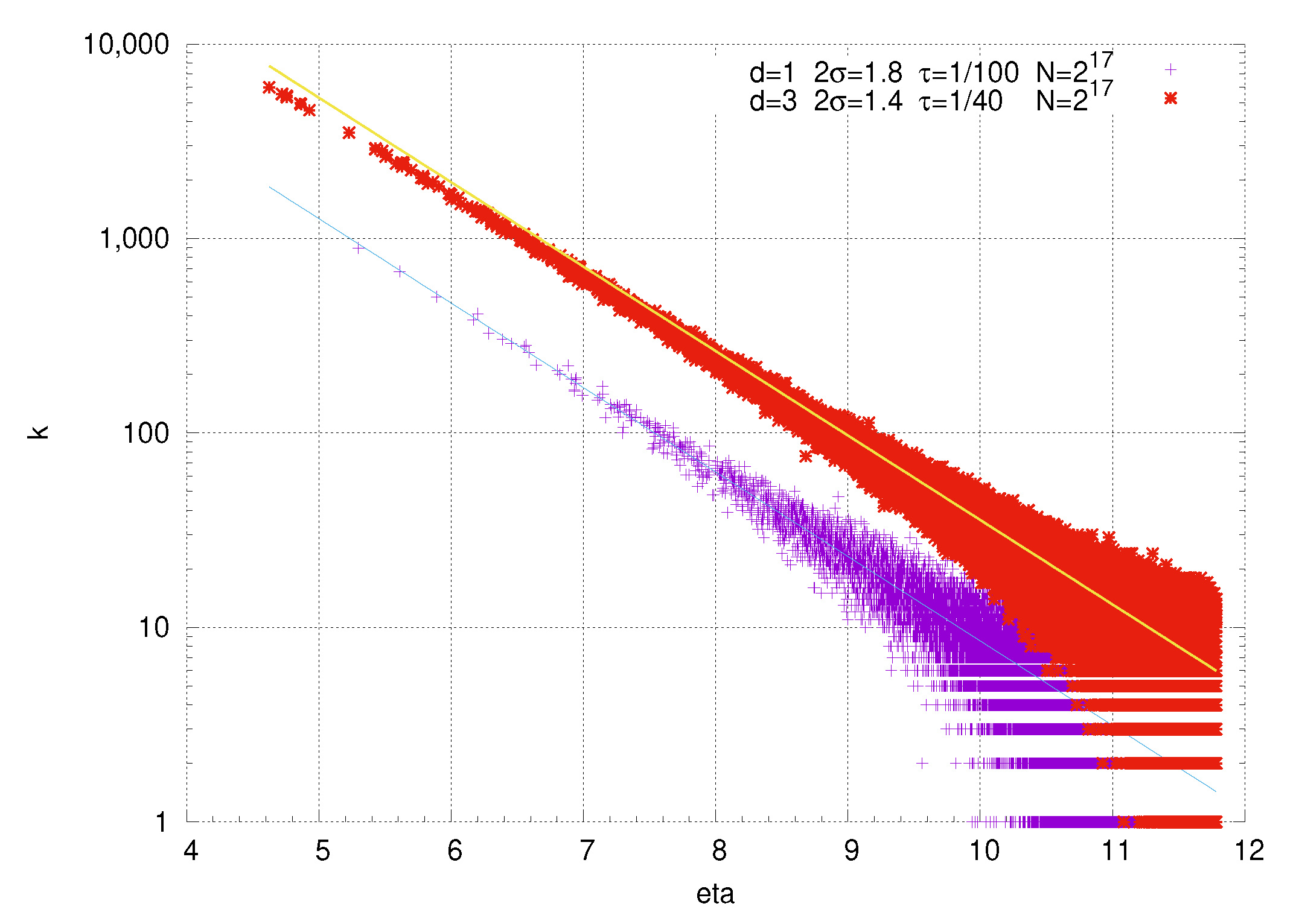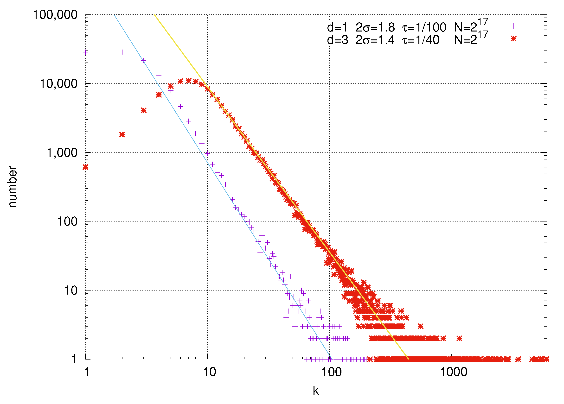Thus, when $\sigma >1$, the nodes are more likely to lie at large radius than they would with a uniform embedding in hyperbolic space, and when $\sigma <1$ they are more likely to lie nearer the origin than in hyperbolic geometry. We will see later that the degree of a node diminishes exponentially with its distance from the origin, and that with larger values of $\sigma$ the model tends to produce networks with a degree distribution which falls off more rapidly at large degree, while with smaller $\sigma$ it produces networks whose degree distribution possesses a ‘fatter tail’ at large degree.

We would like to compute the expected degree sequence of the model, in a limit with $N\to \infty$ and $R=R(N)\to \infty$ as $N\to \infty$. The model is label independent, meaning that, before embedding the vertices into ${\mathbb{H}}^{d+1}$, each vertex is equivalent. To determine the expected degree sequence, it is therefore sufficient to compute the degree distribution of a single vertex, as a function of its embedding coordinates, and then integrate over the hyperbolic ball.

Given that each of the other $N-1$ vertices are randomly distributed in ${\mathbb{H}}^{d+1}$ according to the probability density (3), the expected degree of u will be equal to the connection probability $p_{u,v}$, integrated over ${\mathbb{H}}^{d+1}$, for each of the other $N-1$ vertices. Thus,

$$\langle k_u\rangle =\langle k({\overrightarrow{x}}_u)\rangle =(N-1){\int }_0^R{\int }_0^{\pi }\cdots {\int }_0^{\pi }{\int }_0^{2\pi }\rho (r_v){\rho }_1({\theta }_1)\cdots {\rho }_d({\theta }_d)p_{u,v}d{\theta }_1\cdots d{\theta }_{d}d{r}_v.$$

Since the geometry is independent of angular position, without loss of generality, we can assume our vertex u is embedded at the ‘north pole’ ${\theta }_1=0$, so the relative angle ${\theta }_{u,v}$ between u and any other embedding vertex v is just the angle ${\theta }_1$ of v. (The full hyperbolic geometry is of course completely homogeneous, and thus independent of the radial coordinate as well; however, the presence of the boundary at $r=R$ breaks the radial homogeneity.) Thus,

$$\langle k_u\rangle =\langle k(r_u)\rangle =(N-1){\int }_0^R{\int }_0^{\pi }\rho (r_v){\rho }_1({\theta }_{u,v})p_{u,v}d{\theta }_{u,v}d{r}_v,$$

(4)

where $r_u,r_v$ are the radial coordinates of the vertices $u,v$; ${\theta }_{u,v}$ is the angle between them in the ${\theta }_1$ direction, and ${\rho }_1(\theta )={sin}^{d-1}\theta /I_{d,1}$, with

$$I_{d,1}={\int }_0^{\pi }{sin}^{d-1}\theta d\theta .$$

(5)

To simplify the notation below, we use $\theta$ in place of ${\theta }_{u,v}$.

In the case of $r_u=0$, we have $d_{u,v}=r_v$ and

$$\langle k(0)\rangle =(N-1){\int }_0^R{\int }_0^{\pi }\rho (r_v){\rho }_1({\theta }_{u,v})\frac{1}{1+e^{\frac{r_v-\mu }{T}}}d{\theta }_{u,v}d{r}_v=(N-1){\int }_0^R\rho (r_v)\frac{1}{1+e^{\frac{r_v-\mu }{T}}}d{r}_v.$$

(6)

1.2. Main Results

Let $V_N$ be the vertex set of a random graph G with N vertices, whose elements are randomly distributed with a radially dependent density into a ball of radius R in ${\mathbb{H}}^{d+1}$, $d\ge 1$. Let $D_u$ denote the degree of the vertex u. Throughout $o(1)\to 0$ as $N\to \infty$, unless otherwise indicated.

The main results of this paper are as follows:

Theorem 1.

Let $\tau <1$ and $2\sigma >1$, and k be a non-negative integer, then

$$Pr[D_u=k]=2\sigma {\left(\frac{2\sigma \nu }{2\sigma -1}\frac{c^{*}(\tau ,d)}{I_{d,1}}\right)}^{2\sigma }{k}^{-\gamma }+o(1),$$

where $\gamma =2\sigma +1$, the parameter $\nu >0$ (introduced in Section 2), $c^{*}(\tau ,d)$ is defined by (A3), and $I_{d,1}$ is defined by (5). Here, $o(1)\to 0$ as $k,N\to \infty$.

Theorem 2.

Let $\tau >1$ and $2\sigma >\frac{1}{\tau }$, and k be a non-negative integer, then

$$Pr[D_u=k]=\frac{{(2\sigma \tau )}^{2\sigma \tau +1}{\nu }^{2\sigma \tau }A{(\tau ,d)}^{2\sigma \tau }}{{((2\sigma \tau -1)I_{d,1})}^{\sigma \tau }}{k}^{-\gamma }+o(1),$$

where $\gamma =2\sigma \tau +1$, $\nu >0$, and $A(\tau ,d)$ are defined by (A5). Here, $o(1)\to 0$ as $k,N\to \infty$.

Theorem 3.

Let $\tau <1$, and $\left\{\begin{array}{cc}2\sigma >1\hfill & d=1\hfill \\ 2\sigma >1\hfill & d=2\hfill \\ \frac{4\sigma }{d}>1\hfill & d>2\hfill \end{array}\right.$, for dimension d, for any integer $m\ge 2$ and for any collection of m pairwise distinct vertices $v_i$, $i=1,\cdots m$, their degrees $D_{v_1},\cdots ,D_{v_m}$ are asymptotically independent in the sense that, for any non-negative integers $k_i,i=1,\cdots ,m$,

$$Pr[D_{v_1}=k_1,\cdots ,D_{v_m}=k_m]-\prod _{i=1}^{m}Pr[D_{v_i}=k_i]=o(1).$$

The paper is organized as follows. In Section 1.1 above, we introduce the model. Specifically, we explain the exponential random graph model in hyperbolic space, explain the roles of the parameters, and provide some basic formulas for mean degree. In Section 1.2 above, we state three main theorems. Theorems 1 and 2 state that the probability of degree taking value k for any node, in the limit of large N, takes the form of a power law. Theorem 4 states that the probability of several nodes taking respective k values is asymptotically independent as the number of nodes is growing. In Section 2, we provide some useful preliminary results; in particular, we give an explicit approximation of the hyperbolic distance formula for two points on some conditions, which is superior to previous such expressions. In Section 3, we compute the angular integral, which is the key obstacle that we need to overcome to extend the model to high dimensional hyperbolic space. We use analytic expansion to perform a fine infinitesimal estimation for the angular integral, which could not be done on a computer. We put these computations in Appendix A. Our main proof processes lie in Section 4, Section 5, Section 6 and Section 7. We compute the expected degree of a given vertex as a function of radial coordinate, the mean degree of the network, and the asymptotic distribution of degree for the cases $\tau <1$, $\tau =1$, and $\tau >1$, respectively, in Section 4, Section 5 and Section 6. The proof of Theorem 1 lies in Section 4.1 and the proof of Theorem 2 lies in Section 6.1. In Section 7, we analyze the asymptotic correlations of degree for $\tau <1$ and finally prove Theorem 4.

1.3. Simulations

The Cactus High Performance Computing Framework [19] defines a new paradigm in scientific computing, by defining software in terms of abstract APIs, which allows scientists to construct interoperable modules without having to know the details of function argument specifications from these modules at the outset. One can write toolkits within the framework, which are collections of modules which perform computations in some scientific domain. For the simulation results shown in this paper, we have used a ComplexNetworks toolkit within Cactus, which we hope to be available soon under a freely available open source license.

The ComplexNetworks toolkit is an extension of the CausalSets toolkit [20] which allows many computations involving complex networks to be easily run on distributed memory supercomputers, though the simulations we perform here are small enough to fit on a single 12 core Xeon workstation. The model is implemented by a module which allows direct control of a number of parameters, including $\sigma$, ${\mathcal{R}}_H$, and T, $\mu$ of (1), and N.

2. Preliminaries

We begin with some basic calculations, before attempting to directly evaluate (4).

2.1. Radial Density

Let $\rho (r)=\frac{{sinh}^d(\sigma \zeta r)}{C_d}$ with $C_d={\int }_0^R{sinh}^d(\sigma \zeta r)dr$, $\sigma >0$, $\zeta >0$, integer $d>0$, and $R\gg 1$. Below are some basic calculations which will be very useful in the sequel.

Let $0\le x<R$. Then,

$$\begin{array}{ccc}\hfill {\int }_x^R{sinh}^d(\sigma \zeta r)dr& =& \frac{1}{2^d}{\int }_x^R{(e^{\sigma \zeta r}-e^{-(\sigma \zeta r)})}^{d}dr\hfill \\ & =& \frac{1}{2^d}{\int }_x^R\sum _{i=0}^{d}di{(-1)}^{d-i}{e}^{(2i-d)\sigma \zeta r}dr\hfill \\ & =& \frac{e^{d\sigma \zeta R}}{\sigma \zeta d{2}^d}\left\{\begin{array}{cc}1-e^{-\sigma \zeta (R-x)}+O(e^{-\sigma \zeta (R+x)})\hfill & d=1\hfill \\ 1-e^{-\sigma \zeta d(R-x)}+O((R-x)e^{-2\sigma \zeta R})\hfill & d=2\hfill \\ 1-e^{-\sigma \zeta d(R-x)}+O(e^{-2\sigma \zeta R})\hfill & d>2\hfill \end{array}\right..\hfill \end{array}$$

($O(f(x))$, for some function $f(x)$, means control of growth, i.e., $|O(f(x))|\le C|f(x)|$, for some constant $C>0$, when the variable x is growing.) When $x=0$, we have

$$C_d={\int }_0^R{sinh}^d(\sigma \zeta r)dr=\frac{e^{d\sigma \zeta R}}{\sigma \zeta d{2}^d}\left\{\begin{array}{cc}1-e^{-\sigma \zeta R}+O(e^{-\sigma \zeta R})\hfill & d=1\hfill \\ 1-e^{-\sigma \zeta dR}+O(R{e}^{-2\sigma \zeta R})\hfill & d=2\hfill \\ 1-e^{-\sigma \zeta dR}+O(e^{-2\sigma \zeta R})\hfill & d>2\hfill \end{array}\right.,$$

i.e.,

$$C_d=(1+o_d(1))\frac{e^{d\sigma \zeta R}}{\sigma \zeta d{2}^d},$$

(7)

where

$$o_d(1)=\left\{\begin{array}{cc}O(e^{-\sigma \zeta R})\hfill & d=1\hfill \\ O(R{e}^{-2\sigma \zeta R})\hfill & d=2\hfill \\ O(e^{-2\sigma \zeta R})\hfill & d>2\hfill \end{array}\right..$$

Now, letting $x\gg 1$,

$$\begin{array}{ccc}\hfill {\int }_0^x{sinh}^d(\sigma \zeta r)dr& =& \frac{1}{2^d}{\int }_0^x{(e^{\sigma \zeta r}-e^{-(\sigma \zeta r)})}^{d}dr\hfill \\ & =& \frac{1}{2^d}{\int }_0^x\sum _{i=0}^{d}di{(-1)}^{d-i}{e}^{(2i-d)\sigma \zeta r}dr\hfill \\ & =& \frac{e^{d\sigma \zeta x}}{\sigma \zeta d{2}^d}\left\{\begin{array}{cc}1-2e^{-\sigma \zeta x}+e^{-2\sigma \zeta x}\hfill & d=1\hfill \\ 1+O(x{e}^{-2\sigma \zeta x})\hfill & d=2\hfill \\ 1-\frac{d^2}{d-2}{e}^{-2\sigma \zeta x}+O(e^{-3\sigma \zeta x})\hfill & d>2\hfill \end{array}\right.\hfill \end{array}$$

(8)

For $0\le x<R$, we have

$$\begin{array}{ccc}\hfill {\int }_x^R{sinh}^d(\sigma \zeta r)/C_{d}dr& =& (1+o_d(1))\left\{\begin{array}{cc}1-e^{-\sigma \zeta (R-x)}+O(e^{-\sigma \zeta (R+x)})\hfill & d=1\hfill \\ 1-e^{-2\sigma \zeta (R-x)}+O((R-x)e^{-2\sigma \zeta R})\hfill & d=2\hfill \\ 1-e^{-\sigma \zeta d(R-x)}+O(e^{-2\sigma \zeta R})\hfill & d>2\hfill \end{array}\right.\hfill \\ & =& \left\{\begin{array}{cc}1-e^{-\sigma \zeta (R-x)}+O(e^{-\sigma \zeta R})\hfill & d=1\hfill \\ 1-e^{-2\sigma \zeta (R-x)}+O(R{e}^{-2\sigma \zeta R})\hfill & d=2\hfill \\ 1-e^{-\sigma \zeta d(R-x)}+O(e^{-2\sigma \zeta R})\hfill & d>2\hfill \end{array}\right..\hfill \end{array}$$

(9)

If we set $R=\frac{2}{d\zeta }ln(N/\nu )$, for some $\nu >0$, then

$${\int }_x^R{sinh}^d(\sigma \zeta r)/C_{d}dr=\left\{\begin{array}{cc}1-e^{-\sigma \zeta (R-x)}+O(N^{-2\sigma })\hfill & d=1\hfill \\ 1-e^{-\sigma \zeta d(R-x)}+O(N^{-2\sigma }lnN)\hfill & d=2\hfill \\ 1-e^{-\sigma \zeta d(R-x)}+O(N^{-\frac{4\sigma }{d}})\hfill & d>2\hfill \end{array}\right.,$$

and

$$\rho (r)=(1+o_d(1))\frac{e^{\sigma \zeta dr}{(1-e^{-2\sigma \zeta r})}^d/2^d}{\frac{e^{d\sigma \zeta R}}{\sigma \zeta d{2}^d}}=(1+o_d(1))\sigma \zeta d{e}^{\sigma \zeta d(r-R)}{(1-e^{-2\sigma \zeta r})}^d.$$

(10)

Note that $\nu$ provides some control over the effective density of nodes with respect to the hyperbolic volume measure, though subject to the asymptotic constraint that $R\propto lnN$. Furthermore, we have

$$\rho (r)=\frac{{sinh}^d(\sigma \zeta r)}{C_d}=(1+o(1))\sigma \zeta d{e}^{\sigma \zeta d(r-R)}$$

(11)

uniformly for all r with $R>r>\omega (N)$, where the function $\omega (N)=o(R(N))\to \infty$ as $N\to \infty$. The following Lemma follows immediately from the above.

Lemma 1.

Let $r_v$ be the radial coordinate of the vertex $v\in V_N$. We have

$$\begin{array}{ccc}\hfill Pr[r_v\ge R-x]& =& {\int }_{R-x}^R{sinh}^d(\sigma \zeta r)/C_{d}dr\hfill \\ & =& \left\{\begin{array}{cc}1-e^{-\sigma \zeta x}+O(e^{-\sigma \zeta R})\hfill & d=1\hfill \\ 1-e^{-\sigma \zeta dx}+O(R{e}^{-2\sigma \zeta R})\hfill & d=2\hfill \\ 1-e^{-\sigma \zeta dx}+O(e^{-2\sigma \zeta R})\hfill & d>2\hfill \end{array}\right..\hfill \end{array}$$

If we choose $\frac{d\zeta }{2}R=ln\frac{N}{\nu }$, then

$$\begin{array}{ccc}\hfill Pr[r_v\ge R-x]& =& {\int }_{R-x}^R{sinh}^d(\sigma \zeta r)/C_{d}dr\hfill \\ & =& \left\{\begin{array}{cc}1-e^{-\sigma \zeta x}+O(N^{-2\sigma })\hfill & d=1\hfill \\ 1-e^{-\sigma \zeta dx}+O(N^{-2\sigma }lnN)\hfill & d=2\hfill \\ 1-e^{-\sigma \zeta dx}+O(N^{-\frac{4\sigma }{d}})\hfill & d>2\hfill \end{array}\right.\hfill \end{array}$$

uniformly for all $0\le x\le R.$

Furthermore, letting $r_0=\frac{1}{2\sigma }R+\omega (N)$ with $2\sigma >1$, then

$$\begin{array}{ccc}\hfill Pr[r_v\ge R-r_0]& =& {\int }_{R-r_0}^R{sinh}^d(\sigma \zeta r)/C_{d}dr\hfill \\ & =& \left\{\begin{array}{cc}1-e^{-\sigma \zeta r_0}+O(N^{-2\sigma })\hfill & d=1\hfill \\ 1-e^{-\sigma \zeta d{r}_0}+O(N^{-2\sigma }lnN)\hfill & d=2\hfill \\ 1-e^{-\sigma \zeta d{r}_0}+O(N^{-\frac{4\sigma }{d}})\hfill & d>2\hfill \end{array}\right.\hfill \\ & =& \left\{\begin{array}{cc}1-\frac{\nu }{N}{e}^{-\sigma \zeta \omega (N)}+O(N^{-2\sigma })\hfill & d=1\hfill \\ 1-\frac{\nu }{N}{e}^{-2\sigma \zeta \omega (N)}+O(N^{-2\sigma }lnN)\hfill & d=2\hfill \\ 1-\frac{\nu }{N}{e}^{-\sigma \zeta d\omega (N)}+O(N^{-\frac{4\sigma }{d}})\hfill & d>2\hfill \end{array}\right..\hfill \end{array}$$

Corollary 1.

If $\left\{\begin{array}{cc}2\sigma >1\hfill & d=1\hfill \\ 2\sigma >1\hfill & d=2\hfill \\ \frac{4\sigma }{d}>1\hfill & d>2\hfill \end{array}\right.$, a.a.s. all vertices $v\in V_N$ have $Pr[r_v<R-r_0]=o(\frac{1}{N})$ when $\frac{d\zeta }{2}R=ln\frac{N}{\nu }$.

(Throughout, a.a.s. stands for asymptotically almost surely, i.e., with a probability that tends to 1 as $N\to \infty$.)

Proof. 

$Pr[r_v<R-r_0]=o(\frac{1}{N})$. Thus, $Pr[r_v<R-r_0]={\sum }_{i=1}^{N}Pr[r_v<R-r_0]=o(1)$.  □

2.2. Distance

As mentioned in Section 1.1, the distance $d_{u,v}$ between two vertices u and v is given by the hyperbolic law of cosines

$$cosh\zeta d_{u,v}=cosh\zeta r_{u}cosh\zeta r_v-sinh\zeta r_{u}sinh\zeta r_{v}cos{\theta }_{u,v}.$$

(12)

This hyperbolic distance can be approximated according to the following lemma.

Lemma 2.

Let $h,h_1:\mathbb{N}\to {\mathbb{R}}^{+}$ such that $h(N),h_1(N)\to \infty$ as $N\to \infty$. Let $u,v$ be two distinct points in ${\mathbb{H}}^{d+1}$ with ${\theta }_{u,v}$ denoting their relative angle. Let also ${\hat{\theta }}_{u,v}:={(e^{-2\zeta r_v}+e^{-2\zeta r_u})}^{\frac{1}{2}}.$ If we assume $u,v$ with $r_u+r_v-R\ge h(N)$, then as

$$h_1(N){\hat{\theta }}_{u,v}\le {\theta }_{u,v}\le \pi ,$$

we have

$$d_{u,v}=r_u+r_v+\frac{2}{\zeta }lnsin\left(\frac{{\theta }_{u,v}}{2}\right)+O\left({(\frac{{\hat{\theta }}_{u,v}}{{\theta }_{u,v}})}^2\right),$$

(13)

here $|O\left({(\frac{{\hat{\theta }}_{u,v}}{{\theta }_{u,v}})}^2\right)|\le 3{\pi }^3{(\frac{{\hat{\theta }}_{u,v}}{{\theta }_{u,v}})}^2$ uniformly for all $u,v$ satisfying the above condition. Note that we can take $h_1(N)=h(N)$, for example.

Proof. 

For $r_u+r_v-R\ge h(N)$, we get $r_u,r_v\ge h(N)$, so ${\hat{\theta }}_{u,v}\le \sqrt{2}{e}^{-\zeta h(N)}$. Thus, we may choose $h_1(N)$ to make $h_1(N){\hat{\theta }}_{u,v}<\pi ,$ hence the condition $h_1(N){\hat{\theta }}_{u,v}\le {\theta }_{u,v}\le \pi$ is well defined. Obviously, we can take $h_1(N)=h(N)$ so that $h(N){\hat{\theta }}_{u,v}\ll \pi$.

Next, we prove (13). The right-hand side of (12)

$$\begin{array}{ccc}\hfill cosh\zeta r_{u}cosh\zeta r_v-sinh\zeta r_{u}sinh\zeta r_{v}cos{\theta }_{u,v}& =& \frac{e^{\zeta (r_u+r_v)}}{2}{sin}^2\frac{{\theta }_{u,v}}{2}\left(1+\frac{(1+cos{\theta }_{u,v}){\hat{\theta }}_{u,v}^2}{2{sin}^2\frac{{\theta }_{u,v}}{2}}+e^{-2\zeta (r_u+r_v)}\right)\hfill \\ & =& \frac{e^{\zeta (r_u+r_v)}}{2}{sin}^2\frac{{\theta }_{u,v}}{2}\left(1+O({(\frac{{\hat{\theta }}_{u,v}}{{\theta }_{u,v}})}^2)\right).\hfill \end{array}$$

(14)

Here, $0<O({(\frac{{\hat{\theta }}_{u,v}}{{\theta }_{u,v}})}^2)\le 2{\pi }^2{(\frac{{\hat{\theta }}_{u,v}}{{\theta }_{u,v}})}^2$, and we also make use of Young’s inequality to get

$$e^{-\zeta (r_u+r_v)}=e^{-2\zeta \frac{r_u+r_v}{2}}\le \frac{1}{2}(e^{-2\zeta r_u}+e^{-2\zeta r_v})\le {\hat{\theta }}_{u,v}^2.$$

Thus,

$$\begin{array}{ccc}\hfill cosh\zeta r_{u}cosh\zeta r_v-sinh\zeta r_{u}sinh\zeta r_{v}cos{\theta }_{u,v}& \ge & \frac{1}{{\pi }^2}{\left(\frac{{\theta }_{u,v}}{{\hat{\theta }}_{u,v}}\right)}^2\left(1+O({(\frac{{\hat{\theta }}_{u,v}}{{\theta }_{u,v}})}^2)\right),\hfill \end{array}$$

so from (12), we get

$$e^{\zeta d_{u,v}}\ge \frac{1}{{\pi }^2}{(\frac{{\theta }_{u,v}}{{\hat{\theta }}_{u,v}})}^2\ge \frac{1}{{\pi }^2}{h}_1^2(N).$$

(15)

Furthermore, from (12) and (14), we have

$$\zeta d_{u,v}+ln(1+e^{-2\zeta d_{u,v}})=\zeta (r_u+r_v)+ln{sin}^2\frac{{\theta }_{u,v}}{2}+ln\left(1+O({(\frac{{\hat{\theta }}_{u,v}}{{\theta }_{u,v}})}^2)\right),$$

and, from (15), we have

$$d_{u,v}=(r_u+r_v)+\frac{2}{\zeta }lnsin\frac{{\theta }_{u,v}}{2}+O\left({(\frac{{\hat{\theta }}_{u,v}}{{\theta }_{u,v}})}^2\right),$$

where $|O\left({(\frac{{\hat{\theta }}_{u,v}}{{\theta }_{u,v}})}^2\right)|\le 3{\pi }^2{(\frac{{\hat{\theta }}_{u,v}}{{\theta }_{u,v}})}^2$. Given that

$$h(N){\hat{\theta }}_{u,v}\le {\theta }_{u,v}\le \pi ,$$

(13) is achieved uniformly for all $u,v$ with $r_u+r_v-R\ge h(N)$. Notice that $h(N)$ should grow more slowly than R as $N\to \infty .$  □

3. Angular Integral

The conditional probability ${\hat{p}}_{u,v}$ that a node u at fixed radial coordinate $r_u$ connects to a node v at fixed radius $r_v$ is the connection probability (2) integrated over their possible relative angular separations ${\theta }_1$:

$${\hat{p}}_{u,v}={\int }_0^{\pi }{\rho }_1(\theta )p_{u,v}d\theta ={\int }_0^{\pi }\frac{{sin}^{d-1}\theta }{I_{d,1}}{p}_{u,v}d\theta .$$

(16)

We call this the angular integral, and, to simplify the notation, we will rescale variables as follows:

$$\left({\eta }_u,{\eta }_v,{\mathcal{R}}_H,\tau \right)=\frac{d\zeta }{2}\left(r_u,r_v,R,T\right),$$

and set

$$A_{u,v}:=e^{\frac{d\zeta }{2}(r_u+r_v-R)}=e^{{\eta }_u+{\eta }_v-{\mathcal{R}}_H},$$

so from Lemma 2, if $h_1(N){\hat{\theta }}_{u,v}\le {\theta }_{u,v}\le \pi$ and $r_u+r_v-R\ge h(N)$, then

$$\begin{array}{ccc}\hfill e^{\frac{d_{u,v}-R}{T}}& =& e^{\frac{r_u+r_v-R+\frac{2}{\zeta }lnsin(\frac{{\theta }_{u,v}}{2})+O({(\frac{{\hat{\theta }}_{u,v}}{{\theta }_{u,v}})}^2)}{T}}\hfill \\ & =& e^{\frac{r_u+r_v-R}{T}}{sin}^{\frac{d}{\tau }}(\frac{{\theta }_{u,v}}{2})e^{\frac{O({(\frac{{\hat{\theta }}_{u,v}}{{\theta }_{u,v}})}^2)}{T}}\hfill \\ & =& C_N{e}^{\frac{{\eta }_u+{\eta }_v-{\mathcal{R}}_H}{\tau }}{sin}^{\frac{d}{\tau }}(\frac{{\theta }_{u,v}}{2}),\hfill \end{array}$$

with

$$C_N=1+\frac{O({(\frac{{\hat{\theta }}_{u,v}}{{\theta }_{u,v}})}^2)}{T},$$

so

$$p_{u,v}=\frac{1}{1+e^{\frac{d_{u,v}-R}{T}}}=\frac{1}{1+C_N{e}^{\frac{{\eta }_u+{\eta }_v-{\mathcal{R}}_H}{\tau }}{sin}^{\frac{d}{\tau }}(\frac{\theta }{2})}.$$

Claim 1.

If $r_u+r_v-R\ge \omega (N)$, then $A_{u,v}^{-\frac{1}{d}}\ge \frac{\sqrt{2}}{2}{e}^{\frac{\zeta }{2}\omega (N)}{\hat{\theta }}_{u,v}$.

Proof. 

For ${\hat{\theta }}_{u,v}={(e^{-2\zeta r_v}+e^{-2\zeta r_u})}^{\frac{1}{2}}\le \sqrt{2}max\{e^{-\zeta r_u},e^{-\zeta r_v}\}\le \sqrt{2}{e}^{-\frac{\zeta }{2}\omega (N)}max\{e^{-\frac{\zeta }{2}{r}_u},e^{-\frac{\zeta }{2}{r}_v}\}\le \sqrt{2}{e}^{-\frac{\zeta }{2}\omega (N)}{A}_{u,v}^{-\frac{1}{d}}$, so we get $A_{u,v}^{-\frac{1}{d}}\ge \frac{\sqrt{2}}{2}{e}^{\frac{\zeta }{2}\omega (N)}{\hat{\theta }}_{u,v}.$  □

Now, we set

$${\tilde{\theta }}_{u,v}=\left\{\begin{array}{cc}\frac{A_{u,v}^{-\frac{1}{d}}}{\omega (N)},\hfill & \tau \le 1\hfill \\ \omega (N)A_{u,v}^{-\frac{1}{d}},\hfill & \tau >1\hfill \end{array}\right.,$$

(17)

which means ${\tilde{\theta }}_{u,v}\ge h_1(N){\hat{\theta }}_{u,v}$ as $r_u+r_v-R\ge \omega (N)$, where

$$h_1(N)=\left\{\begin{array}{cc}\frac{\frac{\sqrt{2}}{2}{e}^{\frac{\zeta }{2}\omega (N)}}{\omega (N)},\hfill & \tau \le 1\hfill \\ \frac{\sqrt{2}}{2}{e}^{\frac{\zeta }{2}\omega (N)}\omega (N),\hfill & \tau >1\hfill \end{array}\right..$$

Thus, for $r_u+r_v-R\ge \omega (N)$, we divide the integral (16) as follows:

$${\hat{p}}_{u,v}={\int }_0^{\pi }{\rho }_1(\theta )p_{u,v}d\theta ={\int }_0^{{\tilde{\theta }}_{u,v}}{\rho }_1(\theta )p_{u,v}d\theta +{\int }_{{\tilde{\theta }}_{u,v}}^{\pi }{\rho }_1(\theta )p_{u,v}d\theta .$$

We begin from the first part of the integral

$${\int }_0^{{\tilde{\theta }}_{u,v}}{\rho }_1(\theta )p_{u,v}d\theta \le {\int }_0^{{\tilde{\theta }}_{u,v}}{\rho }_1(\theta )d\theta \le \frac{{\tilde{\theta }}_{u,v}^d}{d{I}_{d,1}}=\left\{\begin{array}{cc}\frac{A_{u,v}^{-1}}{d{I}_{d,1}{\omega }^d(N)},\hfill & \tau \le 1\hfill \\ \frac{{\omega }^d(N)A_{u,v}^{-1}}{d{I}_{d,1}},\hfill & \tau >1\hfill \end{array}\right.=\left\{\begin{array}{cc}o(A_{u,v}^{-1}),\hfill & \tau \le 1\hfill \\ o(A_{u,v}^{-\frac{1}{\tau }}),\hfill & \tau >1\hfill \end{array}\right.$$

(18)

The second part of the integral

$${\int }_{{\tilde{\theta }}_{u,v}}^{\pi }{\rho }_1(\theta )p_{u,v}d\theta ={\int }_{{\tilde{\theta }}_{u,v}}^{\pi }\frac{{\rho }_1(\theta )}{C_N{A}_{u,v}^{\frac{1}{\tau }}{sin}^{\frac{d}{\tau }}(\frac{\theta }{2})+1}d\theta =\frac{1}{I_{d,1}{C}_N{A}_{u,v}^{\frac{1}{\tau }}}{\int }_{{\tilde{\theta }}_{u,v}}^{\pi }\frac{{sin}^{d-1}(\theta )}{{sin}^{\frac{d}{\tau }}(\frac{\theta }{2})+\frac{1}{C_N{A}_{u,v}^{\frac{1}{\tau }}}}d\theta .$$

(19)

Notice the estimation $I=\delta {\int }_0^{\pi }\frac{{sin}^{d-1}\theta d\theta }{\delta +{sin}^{\frac{d}{\tau }}(\frac{\theta }{2})}$ in Appendix A, for the integral

$$\frac{1}{C_N{A}_{u,v}^{\frac{1}{\tau }}}{\int }_{{\tilde{\theta }}_{u,v}}^{\pi }\frac{{sin}^{d-1}(\theta )}{{sin}^{\frac{d}{\tau }}(\frac{\theta }{2})+\frac{1}{C_N{A}_{u,v}^{\frac{1}{\tau }}}}d\theta =\frac{1}{C_N{A}_{u,v}^{\frac{1}{\tau }}}{\int }_0^{\pi }\frac{{sin}^{d-1}(\theta )}{{sin}^{\frac{d}{\tau }}(\frac{\theta }{2})+\frac{1}{C_N{A}_{u,v}^{\frac{1}{\tau }}}}d\theta -\frac{1}{C_N{A}_{u,v}^{\frac{1}{\tau }}}{\int }_0^{{\tilde{\theta }}_{u,v}}\frac{{sin}^{d-1}(\theta )}{{sin}^{\frac{d}{\tau }}(\frac{\theta }{2})+\frac{1}{C_N{A}_{u,v}^{\frac{1}{\tau }}}}d\theta .$$

Setting $\delta =\frac{1}{C_N{A}_{u,v}^{\frac{1}{\tau }}}$, and taking account of (18), we have

• for $\tau <1$,

  $$\frac{1}{C_N{A}_{u,v}^{\frac{1}{\tau }}}{\int }_0^{\pi }\frac{{sin}^{d-1}(\theta )}{{sin}^{\frac{d}{\tau }}(\frac{\theta }{2})+\frac{1}{C_N{A}_{u,v}^{\frac{1}{\tau }}}}d\theta =c^{*}(\tau ,d)C_N^{-\tau }{A}_{u,v}^{-1}+o(A_{u,v}^{-1})=c^{*}(\tau ,d)A_{u,v}^{-1}+o(A_{u,v}^{-1}),$$

  since $C_N=1+o(1)$,
• for $\tau =1$,

  $$\begin{array}{ccc}\hfill \frac{1}{C_N{A}_{u,v}^{\frac{1}{\tau }}}{\int }_0^{\pi }\frac{{sin}^{d-1}(\theta )}{{sin}^{\frac{d}{\tau }}(\frac{\theta }{2})+\frac{1}{C_N{A}_{u,v}^{\frac{1}{\tau }}}}d\theta & =& \frac{2^d}{d}{(C_N{A}_{u,v})}^{-1}ln(C_N{A}_{u,v})+o({(C_N{A}_{u,v})}^{-1}ln(C_N{A}_{u,v}))\hfill \\ & =& \frac{2^d}{d}{A}_{u,v}^{-1}ln{A}_{u,v}+o(A_{u,v}^{-1}ln{A}_{u,v}),\hfill \end{array}$$
• and for $\tau >1$,

  $$\frac{1}{C_N{A}_{u,v}^{\frac{1}{\tau }}}{\int }_0^{\pi }\frac{{sin}^{d-1}(\theta )}{{sin}^{\frac{d}{\tau }}(\frac{\theta }{2})+\frac{1}{C_N{A}_{u,v}^{\frac{1}{\tau }}}}d\theta =A(\tau ,d){(C_N{A}_{u,v}^{\frac{1}{\tau }})}^{-1}+o({(C_N{A}_{u,v}^{\frac{1}{\tau }})}^{-1})=A(\tau ,d)A_{u,v}^{-\frac{1}{\tau }}+o(A_{u,v}^{-\frac{1}{\tau }}).$$

Finally, we get the angular integral estimation:

Lemma 3.

$${\hat{p}}_{u,v}={\int }_0^{\pi }{\rho }_1(\theta )p_{u,v}d\theta =\left\{\begin{array}{cc}\frac{c^{*}(\tau ,d)}{I_{d,1}}{A}_{u,v}^{-1}+o(A_{u,v}^{-1})\hfill & \tau <1\hfill \\ \frac{2^d}{d{I}_{d,1}}{A}_{u,v}^{-1}ln{A}_{u,v}+o(A_{u,v}^{-1}ln{A}_{u,v})\hfill & \tau =1\hfill \\ \frac{A(\tau ,d)}{I_{d,1}}{A}_{u,v}^{-\frac{1}{\tau }}+o(A_{u,v}^{-\frac{1}{\tau }})\hfill & \tau >1\hfill \end{array}\right.=\left\{\begin{array}{cc}(1+o(1))\frac{c^{*}(\tau ,d)}{I_{d,1}}{A}_{u,v}^{-1}\hfill & \tau <1\hfill \\ (1+o(1))\frac{2^d}{d{I}_{d,1}}{A}_{u,v}^{-1}ln{A}_{u,v}\hfill & \tau =1\hfill \\ (1+o(1))\frac{A(\tau ,d)}{I_{d,1}}{A}_{u,v}^{-\frac{1}{\tau }}\hfill & \tau >1\hfill \end{array}\right.$$

assuming $r_u+r_v-R\ge \omega (N)$.

4. Expected Degree Distribution for $\tau <1$

We are now in a position to compute the expected degree of node u. Let $I_{u,v}$ be an indicator random variable which is 1 when there is an edge between nodes u and v in the graph, and 0, otherwise. Recall that the coordinates of u are $(r_u,{\overrightarrow{\theta }}_u)$. Below, we assume $r_u>\omega (N)$. Now,

$$\begin{array}{ccc}\hfill Pr[I_{u,v}=1|r_u,{\overrightarrow{\theta }}_u]& =& {\int }_0^R{\hat{p}}_{u,v}\rho (r_v)d{r}_v\hfill \\ & =& {\int }_0^{R-r_u+\omega (N)}{\hat{p}}_{u,v}\rho (r_v)d{r}_v+{\int }_{R-r_u+\omega (N)}^R{\hat{p}}_{u,v}\rho (r_v)d{r}_v.\hfill \end{array}$$

(20)

Notice that $Pr[I_{u,v}=1|r_u,{\overrightarrow{\theta }}_u]$ depends only on the radius $r_u$ (or rescaled radius coordinate ${\eta }_u$), as one would expect from spherical symmetry. We therefore omit the ${\overrightarrow{\theta }}_u$ in $Pr[I_{u,v}=1|r_u,{\overrightarrow{\theta }}_u]$ and write $\langle k(r_u)\rangle$ instead of $\langle k({\overrightarrow{x}}_u)\rangle$. From (4),

$$\langle k(r_u)\rangle =(N-1)Pr[I_{u,v}=1|r_u].$$

We estimate the first part of the integral (20). From (7), (8) and $R-r_u+\omega (N)\to \infty$ as $N\to \infty$, we have

$$\begin{array}{ccc}\hfill {\int }_0^{R-r_u+\omega (N)}{\hat{p}}_{u,v}\rho (r_v)d{r}_v& \le & {\int }_0^{R-r_u+\omega (N)}\frac{{sinh}^d(\sigma \zeta r_v)}{C_d}d{r}_v\hfill \\ & =& \frac{e^{d\sigma \zeta (R-r_u+\omega (N))}(1+o(1))}{e^{\sigma \zeta dR}(1+o_d(1))}\hfill \\ & =& e^{\sigma \zeta d\omega (N)}{e}^{-2\sigma {\eta }_u}(1+o(1)).\hfill \end{array}$$

(21)

Next, we estimate the second part of the integral (20). From Lemma 3 and (11), we have

$$\begin{array}{cc}\hfill {\int }_{R-r_u+\omega (N)}^R{\hat{p}}_{u,v}\rho (r_v)d{r}_v& =(1+o(1))\frac{c^{*}(\tau ,d)}{I_{d,1}}{\int }_{R-r_u+\omega (N)}^R{A}_{u,v}^{-1}\rho (r_v)d{r}_v\hfill \\ \hfill & =(1+o(1))\frac{c^{*}(\tau ,d)}{I_{d,1}}{e}^{-({\eta }_u-{\mathcal{R}}_H)}{\int }_{{\mathcal{R}}_H-{\eta }_u+\frac{d\zeta }{2}\omega (N)}^{{\mathcal{R}}_H}{e}^{-\eta }2\sigma e^{2\sigma (\eta -{\mathcal{R}}_H)}d\eta \hfill \\ \hfill & =(1+o(1))\frac{c^{*}(\tau ,d)}{I_{d,1}}{e}^{-{\eta }_u}·\left\{\begin{array}{cc}\frac{2\sigma }{2\sigma -1}(1-e^{(2\sigma -1)(\frac{d\zeta }{2}\omega (N)-{\eta }_u)})\hfill & 2\sigma \ne 1\hfill \\ ({\eta }_u-\frac{d\zeta }{2}\omega (N))\hfill & 2\sigma =1\hfill \end{array}\right.\hfill \end{array}$$

(22)

where $\overline{\rho }(\eta )=\frac{2}{d\zeta }\rho (\frac{2}{d\zeta }\eta )$.

4.1. $\tau <1$ and $2\sigma >1$

4.1.1. Mean Degree

We first compute the mean degree for $\tau <1$ and $2\sigma >1$, with ${\mathcal{R}}_H=ln\frac{N}{\nu }$.

$$\begin{array}{ccc}\hfill \langle k\rangle & =& {\int }_{\omega (N)}^R\rho (r)\langle k(r)\rangle dr+{\int }_0^{\omega (N)}\rho (r)\langle k(r)\rangle dr\hfill \\ & =& (N-1){\int }_{\omega (N)}^R\rho (r_u)\left[{\int }_0^{R-r_u+\omega (N)}{\hat{p}}_{u,v}\rho (r_v)d{r}_v+{\int }_{R-r_u+\omega (N)}^R{\hat{p}}_{u,v}\rho (r_v)d{r}_v\right]d{r}_u+{\int }_0^{\omega (N)}\rho (r)\langle k(r)\rangle dr.\hfill \end{array}$$

(23)

From (21),

$$\begin{array}{ccc}\hfill I_1& :=& (N-1){\int }_{\omega (N)}^R\rho (r_u){\int }_0^{R-r_u+\omega (N)}{\hat{p}}_{u,v}\rho (r_v)d{r}_{v}d{r}_u\hfill \\ & \le & (N-1){\int }_{\frac{d\zeta }{2}\omega (N)}^{{\mathcal{R}}_H}(1+o(1))2\sigma e^{2\sigma (\eta -{\mathcal{R}}_H)}{e}^{\sigma \zeta d\omega (N)}{e}^{-2\sigma \eta }(1+o(1))d\eta \hfill \\ & =& (N-1)(1+o(1))2\sigma ({\mathcal{R}}_H-\frac{d\zeta }{2}\omega (N))e^{-2\sigma {\mathcal{R}}_H}{e}^{\sigma \zeta d\omega (N)}\hfill \\ & =& o(1).\hfill \end{array}$$

(24)

From (22),

$$\begin{array}{ccc}\hfill I_2& :=& (N-1){\int }_{\omega (N)}^R\rho (r_u){\int }_{R-r_u+\omega (N)}^R{\hat{p}}_{u,v}\rho (r_v)d{r}_{v}d{r}_u\hfill \\ & =& (N-1){\int }_{\frac{d\zeta }{2}\omega (N)}^{{\mathcal{R}}_H}(1+o(1))2\sigma e^{2\sigma (\eta -{\mathcal{R}}_H)}(1+o(1))\frac{2\sigma }{2\sigma -1}\frac{c^{*}(\tau ,d)}{I_{d,1}}{e}^{-\eta }(1-e^{\frac{(2\sigma -1)d\zeta }{2}\omega (N)}{e}^{-(2\sigma -1)\eta })d\eta \hfill \\ & =& (1+o(1))\frac{{(2\sigma )}^2}{{(2\sigma -1)}^2}\frac{\nu c^{*}(\tau ,d)}{I_{d,1}}.\hfill \end{array}$$

(25)

From (7) and (8),

$$\begin{array}{ccc}\hfill I_3& :=& {\int }_0^{\omega (N)}\rho (r)\langle k(r)\rangle dr\hfill \\ & \le & (N-1){\int }_0^{\omega (N)}\rho (r)dr\hfill \\ & =& (N-1)(1+o(1))e^{2\sigma (\frac{d\zeta }{2}\omega (N)-{\mathcal{R}}_H)}\hfill \\ & =& o(1).\hfill \end{array}$$

(26)

Thus, we have

$$\langle k\rangle =I_1+I_2+I_3=\frac{{(2\sigma )}^2}{{(2\sigma -1)}^2}\frac{\nu c^{*}(\tau ,d)}{I_{d,1}}+o(1).$$

(27)

4.1.2. Asymptotic Degree Distribution

Now, we compute the asymptotic degree distribution. When $r_u\gg \omega (N)$, we have

$${\int }_0^{R-r_u+\omega (N)}{\hat{p}}_{u,v}\rho (r_v)d{r}_v\le o(1)e^{-{\eta }_u}$$

from (21) and ${\int }_{R-r_u+\omega (N)}^R{\hat{p}}_{u,v}\rho (r_v)d{r}_v=(1+o(1))\frac{2\sigma }{2\sigma -1}\frac{c^{*}(\tau ,d)}{I_{d,1}}{e}^{-{\eta }_u}$ from (22). Thus,

$$Pr[I_{u,v}=1|r_u]=(1+o(1))K{e}^{-{\eta }_u},$$

(28)

where $K=\frac{2\sigma }{2\sigma -1}\frac{c^{*}(\tau ,d)}{I_{d,1}}.$ When $r_u\ge \frac{R}{2}+\omega (N)$, we have $o(1)\to 0$ as $N\to \infty$ uniformly. Furthermore, we have

$$\langle k(r_u)\rangle =(N-1)Pr[I_{u,v}=1|r_u]=(N-1)(1+o(1))K{e}^{-{\eta }_u}.$$

(29)

Equation (29) is compared with simulation in Figure 1.

$D_u={\sum }_{v\in V_N^u}{I}_{u,v}$, where $V_N^u=V_N\backslash \left\{u\right\}$, is the number of connections to the vertex u, i.e., its degree. In general, it depends on the coordinates of u: $r_u$ and ${\overrightarrow{\theta }}_u$; however, due to the angular symmetry, only the $r_u$ dependence remains. The quantities ${\left\{I_{u,v}\right\}}_{v\in V_N^u}$ are a family of independent and identically distributed indicator random variables, whose expectation values are given by $()$. Let ${\hat{D}}_u$ be a Poisson random variable with parameter equal to $T_u:={\sum }_{v\in V_N^u}Pr[I_{u,v}=1|r_u]$, and $T_u=\langle k(r_u)\rangle$ from (29). Recall that the total variation distance $d_{TV}(X_1,X_2)$ between two non-negative discrete random variables is defined as $\frac{1}{2}{\sum }_{k=0}^{\infty }|Pr[X_1=k]-Pr[X_2=k]|$.

Claim 2.

If $\frac{d\zeta }{2}R=ln\frac{N}{\nu }$, then

$$d_{TV}(D_u,{\hat{D}}_u)=o(1),$$

uniformly for all $r_u\ge \frac{R}{2}+\omega (N)$.

Proof. 

From Theorem 2.10 in [21]

$$d_{TV}(D_u,{\hat{D}}_u)\le \sum _{v\in V_N^u}Pr{[I_{u,v}=1|r_u]}^2\le (N-1){((1+o(1))K{e}^{-{\eta }_u})}^2=o(1).$$

 □

Using the above claim, we have, for any $k>0$, the probability that the vertex u has k connections is

$$\begin{array}{ccc}\hfill Pr[D_u=k]& =& {\int }_0^R{\int }_{{\overrightarrow{\theta }}_u}Pr[D_u=k|r_u,{\overrightarrow{\theta }}_u]\rho (r_u){\rho }_{\theta }({\overrightarrow{\theta }}_u)d{r}_{u}d{\overrightarrow{\theta }}_u\hfill \\ & =& {\int }_0^R{\int }_{{\overrightarrow{\theta }}_u}Pr[D_u=k|r_u]\rho (r_u){\rho }_{\theta }({\overrightarrow{\theta }}_u)d{r}_{u}d{\overrightarrow{\theta }}_u\hfill \\ & =& {\int }_0^{\frac{R}{2}+\omega (N)}Pr[D_u=k|r_u]\rho (r_u)d{r}_u+{\int }_{\frac{R}{2}+\omega (N)}^{R}Pr[D_u=k|r_u]\rho (r_u)d{r}_u\hfill \\ & =& o(1)+{\int }_{\frac{R}{2}+\omega (N)}^{R}Pr[{\hat{D}}_u=k|r_u]\rho (r_u)d{r}_u\hfill \end{array}$$

(30)

since

$${\int }_0^{\frac{R}{2}+\omega (N)}Pr[D_u=k|r_u]\rho (r_u)d{r}_u\le {\int }_0^{\frac{R}{2}+\omega (N)}\rho (r_u)d{r}_u=(1+o(1))e^{\sigma \zeta d(\omega (N)-\frac{R}{2})}=o(1)$$

(31)

from (7) and (8). Taking the specific expression of the Poisson distribution into (30) and rescaling the integral, we have

$$Pr[D_u=k]={\int }_{\frac{{\mathcal{R}}_H}{2}+\frac{d\zeta }{2}\omega (N)}^{{\mathcal{R}}_H}\frac{1}{k!}{e}^{-(1+o(1))K(N-1)e^{-{\eta }_u}}{((1+o(1))K(N-1)e^{-{\eta }_u})}^k\overline{\rho }({\eta }_u)d{\eta }_u+o(1),$$

(32)

where $\overline{\rho }({\eta }_u)=(1+o(1))2\sigma e^{2\sigma ({\eta }_u-{\mathcal{R}}_H)}$ from (11). On the other hand,

$${\int }_0^{\frac{{\mathcal{R}}_H}{2}+\frac{d\zeta }{2}\omega (N)}\frac{1}{k!}{e}^{-(1+o(1))K(N-1)e^{-{\eta }_u}}{((1+o(1))K(N-1)e^{-{\eta }_u})}^k(1+o(1))2\sigma e^{2\sigma ({\eta }_u-{\mathcal{R}}_H)}d{\eta }_u=o(1).$$

(33)

Thus,

$$Pr[D_u=k]={\int }_0^{{\mathcal{R}}_H}\frac{1}{k!}{e}^{-(1+o(1))K(N-1)e^{-{\eta }_u}}{((1+o(1))K(N-1)e^{-{\eta }_u})}^k(1+o(1))2\sigma e^{2\sigma ({\eta }_u-{\mathcal{R}}_H)}d{\eta }_u+o(1).$$

(34)

Changing the integration variable to $x=K(N-1)e^{-{\eta }_u}$,

$$\begin{array}{ccc}\hfill Pr[D_u=k]& =& -(1+o(1))2\sigma {(K(N-1))}^{2\sigma }{e}^{-2\sigma {\mathcal{R}}_H}{\int }_{K(N-1)}^{K(N-1)e^{-{\mathcal{R}}_H}}\frac{1}{k!}{((1+o(1))x)}^k{x}^{-(2\sigma +1)}{e}^{-(1+o(1))x}dx+o(1)\hfill \\ & =& (1+o(1))2\sigma {(K(N-1))}^{2\sigma }{(\nu /N)}^{2\sigma }{\int }_{K(N-1)\nu /N}^{K(N-1)}\frac{1}{k!}{x}^{k-(2\sigma +1)}{e}^{-x}dx+o(1)\hfill \\ & =& (1+o(1))2\sigma {\nu }^{2\sigma }{(\frac{K(N-1)}{N})}^{2\sigma }\left\{{\int }_0^{\infty }-{\int }_0^{\frac{\nu K(N-1)}{N}}-{\int }_{K(N-1)}^{\infty }\right\}\frac{1}{k!}{x}^{k-(2\sigma +1)}{e}^{-x}dx+o(1)\hfill \\ & =& (1+o(1))\frac{{(\frac{2\sigma \nu }{2\sigma -1}\frac{c^{*}(\tau ,d)}{I_{d,1}})}^{2\sigma }{(\frac{N-1}{N})}^{2\sigma }\Gamma (k-2\sigma )}{k!}+O\left(\frac{{(\nu K)}^k}{k!}\right)+o(1)\hfill \\ & =& 2\sigma {\left(\frac{2\sigma \nu }{2\sigma -1}\frac{c^{*}(\tau ,d)}{I_{d,1}}\right)}^{2\sigma }{k}^{-\gamma }+o_{k,N}(1),\hfill \end{array}$$

(35)

where $o_{k,N}(1)\to 0,$ as $k,N\to \infty$, $\gamma =2\sigma +1,$ and we used that $\frac{\Gamma (k-2\sigma )}{k!}\to k^{-\gamma }$ as $k\to \infty$. Above, we made use of the mean value theorem to assert that

$$\left|\frac{{((1+o(1))x)}^k{e}^{-(1+o(1))x}}{k!}-\frac{x^k{e}^{-x}}{k!}\right|=\left|\frac{{\xi }^{k-1}{e}^{-\xi }(k-\xi )}{k!}o(1)x\right|\le 2\left|o(1)x\right|.$$

(36)

Theorem 1 follows from (35).

The power law distribution in (35) is compared with samples from the model’s degree distribution in Figure 2.

4.2. $\tau <1$ and $2\sigma =1$

4.2.1. Mean Degree

First, we analyze the mean degree when ${\mathcal{R}}_H=ln\frac{N}{\nu }$. From (23), we again compute the three parts below:

$$\begin{array}{ccc}\hfill I_1& =& (N-1){\int }_{\omega (N)}^R\rho (r_u){\int }_0^{R-r_u+\omega (N)}{\hat{p}}_{u,v}\rho (r_v)d{r}_{v}d{r}_u\hfill \\ & \le & (N-1){\int }_{\frac{d\zeta }{2}\omega (N)}^{{\mathcal{R}}_H}\overline{\rho }(\eta )e^{\sigma \zeta d\omega (N)}{e}^{-\eta }(1+o(1))d\eta \hfill \\ & =& (N-1){\int }_{\frac{d\zeta }{2}\omega (N)}^{{\mathcal{R}}_H}(1+o(1))e^{(\eta -{\mathcal{R}}_H)}{e}^{\sigma \zeta d\omega (N)}{e}^{-\eta }(1+o(1))d\eta \hfill \\ & =& (1+o(1))\nu ({\mathcal{R}}_H-\frac{d\zeta }{2}\omega (N))e^{\frac{d\zeta }{2}\omega (N)}.\hfill \end{array}$$

From (22),

$$\begin{array}{ccc}\hfill I_2& =& (N-1){\int }_{\omega (N)}^R\rho (r_u){\int }_{R-r_u+\omega (N)}^R{\hat{p}}_{u,v}\rho (r_v)d{r}_{v}d{r}_u\hfill \\ & =& (N-1){\int }_{\frac{d\zeta }{2}\omega (N)}^{{\mathcal{R}}_H}(1+o(1))e^{(\eta -{\mathcal{R}}_H)}(1+o(1))\frac{c^{*}(\tau ,d)}{I_{d,1}}{e}^{-\eta }(\eta -\frac{d\zeta }{2}\omega (N))d\eta \hfill \\ & =& (1+o(1))\frac{\nu c^{*}(\tau ,d)}{I_{d,1}}\frac{{({\mathcal{R}}_H-\frac{d\zeta }{2}\omega (N))}^2}{2}.\hfill \end{array}$$

From (7) and (8),

$$\begin{array}{ccc}\hfill I_3& =& {\int }_0^{\omega (N)}\rho (r)\langle k(r)\rangle dr\hfill \\ & \le & (N-1){\int }_0^{\omega (N)}\rho (r)dr\hfill \\ & =& (1+o(1))e^{\frac{d\zeta }{2}\omega (N)}.\hfill \end{array}$$

If we choose $\omega (N)$ satisfying $e^{\frac{d\zeta }{2}\omega (N)}=o(\mathcal{R})$, it is easy to see that mean degree $\langle k\rangle =(1+o(1))\frac{\nu c^{*}(\tau ,d)}{I_{d,1}}\frac{{({\mathcal{R}}_H-\frac{d\zeta }{2}\omega (N))}^2}{2}$ will go to infinity as $N\to \infty$.

4.2.2. Asymptotic Degree Distribution

Next, we compute the asymptotic degree distribution. When ${\eta }_u\ge \frac{2}{3}{\mathcal{R}}_H+\frac{d\zeta }{2}\omega (N)$, we have

$${\int }_0^{R-r_u+\omega (N)}{\hat{p}}_{u,v}\rho (r_v)d{r}_v\le e^{\frac{d\zeta }{2}\omega (N)}{e}^{-{\eta }_u}(1+o(1))=o({\eta }_u{e}^{-{\eta }_u})$$

from (21) when we choose $\omega (N)$ satisfying $e^{\frac{d\zeta }{2}\omega (N)}=o(\mathcal{R})$, and

$${\int }_{R-r_u+\omega (N)}^R{\hat{p}}_{u,v}\rho (r_v)d{r}_v=(1+o(1))\frac{c^{*}(\tau ,d)}{I_{d,1}}{e}^{-{\eta }_u}({\eta }_u-\frac{d\zeta }{2}\omega (N))=(1+o(1))\frac{c^{*}(\tau ,d)}{I_{d,1}}{\eta }_u{e}^{-{\eta }_u}$$

from (22). Thus,

$$Pr[I_{u,v}=1|r_u]=(1+o(1))\frac{c^{*}(\tau ,d)}{I_{d,1}}{\eta }_u{e}^{-{\eta }_u}$$

(37)

uniformly for all ${\eta }_u\ge \frac{2}{3}{\mathcal{R}}_H+\frac{d\zeta }{2}\omega (N)$. Similarly to Claim 2, we have

$$\begin{array}{ccc}\hfill d_{TV}(D_u,{\hat{D}}_u)& \le & \sum _{v\in V_N^u}Pr{[I_{u,v}=1|r_u]}^2\lesssim (N-1){({\eta }_u{e}^{-{\eta }_u})}^2\hfill \\ & \lesssim & (N-1)\frac{{\mathcal{R}}_H^2}{e^{\frac{4}{3}{\mathcal{R}}_H+d\zeta \omega (N)}}=o(1),\hfill \end{array}$$

if we choose ${\mathcal{R}}_H=ln\frac{N}{\nu }$. The degree distribution is

$$Pr[D_u=k]={\int }_{\frac{2}{3}{\mathcal{R}}_H+\frac{d\zeta }{2}\omega (N)}^{{\mathcal{R}}_H}\frac{1}{k!}{e}^{-(N-1)(1+o(1))\frac{c^{*}(\tau ,d)}{I_{d,1}}{\eta }_u{e}^{-{\eta }_u}}{((N-1)(1+o(1))\frac{c^{*}(\tau ,d)}{I_{d,1}}{\eta }_u{e}^{-{\eta }_u})}^k(1+o(1))e^{{\eta }_u-{\mathcal{R}}_H}d{\eta }_u+o(1).$$

Figure 3 gives the tendency of $Pr[D_u=k]$ as N is increasing. If we choose ${\mathcal{R}}_H=ln\frac{N}{\nu }$, then

$$(N-1)\frac{c^{*}(\tau ,d)}{I_{d,1}}{\eta }_u{e}^{-{\eta }_u}\gtrsim \frac{d\zeta }{2}\omega (N)$$

uniformly for all

$$\frac{2}{3}{\mathcal{R}}_H+\frac{d\zeta }{2}\omega (N)<\eta <{\mathcal{R}}_H.$$

Since $\frac{e^{-x}{x}^k}{k!}$ is decreasing to 0 when $x>k$, then for any $ϵ>0$, if N is large enough, then

$$\frac{1}{k!}{e}^{-(N-1)(1+o(1))\frac{c^{*}(\tau ,d)}{I_{d,1}}{\eta }_u{e}^{-{\eta }_u}}{\left((N-1)(1+o(1))\frac{c^{*}(\tau ,d)}{I_{d,1}}{\eta }_u{e}^{-{\eta }_u}\right)}^k<ϵ$$

uniformly about $(\frac{2}{3}{\mathcal{R}}_H+\frac{d\zeta }{2}\omega (N))<\eta <{\mathcal{R}}_H$. Therefore,

$$Pr[D_u=k]\le ϵ(1+o(1))+o(1),$$

which means that the k-degree probability $Pr[D_u=k]$ will be very small when N is large enough, for any fixed $k\ge 0$. Note that, comparing the k-degree probability with the mean degree, we see that the rates at which the k-degree probabilities go to zero as $N\to \infty$ cannot be uniform. It would be interesting to study the behavior of the limiting degree distribution as $k\to \infty$.

5. Expected Degree Distribution for $\mathit{\tau }\mathbf{=}\mathbf{1}$

Firstly, we compute

$${\int }_{R-r_u+\omega (N)}^R{\hat{p}}_{u,v}\rho (r_v)d{r}_v.$$

From (11) and Lemma 3, we take ${\hat{p}}_{u,v}=(1+o(1))\frac{2^d}{d{I}_{d,1}}{A}_{u,v}^{-1}ln{A}_{u,v}$ into the above integral, so that

$$\begin{array}{cc}\hfill {\int }_{R-r_u+\omega (N)}^R{\hat{p}}_{u,v}\rho (r_v)d{r}_v& =(1+o(1))\frac{2^d}{d{I}_{d,1}}{\int }_{R-r_u+\omega (N)}^R\sigma \zeta d{e}^{\sigma \zeta d(r-R)}{A}_{u,v}^{-1}ln{A}_{u,v}d{r}_v\hfill \\ \hfill & =(1+o(1))\frac{2\sigma 2^d}{d{I}_{d,1}}{\int }_{{\mathcal{R}}_H-{\eta }_u+\frac{d\zeta }{2}\omega (N)}^{{\mathcal{R}}_H}({\eta }_u+\eta -{\mathcal{R}}_H)e^{{\mathcal{R}}_H-{\eta }_u-\eta }{e}^{2\sigma (\eta -{\mathcal{R}}_H)}d\eta \hfill \\ \hfill & =(1+o(1))\frac{2\sigma 2^d}{d{I}_{d,1}}{e}^{(1-2\sigma ){\mathcal{R}}_H-{\eta }_u}{\int }_{{\mathcal{R}}_H-{\eta }_u+\frac{d\zeta }{2}\omega (N)}^{{\mathcal{R}}_H}({\eta }_u+\eta -{\mathcal{R}}_H)e^{(2\sigma -1)\eta }d\eta \hfill \\ \hfill & =\left\{\begin{array}{cc}(1+o(1))\frac{2\sigma 2^d}{d{I}_{d,1}}{e}^{-{\eta }_u}\left[\frac{{\eta }_u}{2\sigma -1}-\frac{\frac{d\zeta }{2}\omega (N)e^{(2\sigma -1)(\frac{d\zeta }{2}\omega (N)-{\eta }_u)}}{2\sigma -1}-\frac{1}{{(2\sigma -1)}^2}+\frac{e^{(2\sigma -1)(\frac{d\zeta }{2}\omega (N)-{\eta }_u)}}{{(2\sigma -1)}^2}\right]\hfill & 2\sigma \ne 1,\hfill \\ (1+o(1))\frac{2^d}{d{I}_{d,1}}{e}^{-{\eta }_u}\frac{{\eta }_u^2-{(\frac{d\zeta \omega (N)}{2})}^2}{2}\hfill & 2\sigma =1.\hfill \end{array}\right.\hfill \end{array}$$

(38)

5.1. $\tau =1$ and $2\sigma >1$

5.1.1. Asymptotic Degree Distribution

If $2\sigma >1$, when $r_u\gg \omega (N)$, we have ${\int }_0^{R-r_u+\omega (N)}{\hat{p}}_{u,v}\rho (r_v)d{r}_v\le o(1)e^{-{\eta }_u}$ from (21) and

$${\int }_{R-r_u+\omega (N)}^R{\hat{p}}_{u,v}\rho (r_v)d{r}_v=(1+o(1))\frac{2\sigma 2^d}{(2\sigma -1)d{I}_{d,1}}{\eta }_u{e}^{-{\eta }_u}$$

from (38), so

$$Pr[I_{u,v}=1|r_u]=(1+o(1))\frac{2\sigma 2^d}{(2\sigma -1)d{I}_{d,1}}{\eta }_u{e}^{-{\eta }_u}.$$

(39)

For all $r_u\ge \frac{R}{2}+\omega (N)$, we have $o(1)\to 0$ as $N\to \infty$ uniformly. From this, the mean degree

$$\langle k({\eta }_u)\rangle =(N-1)Pr[I_{u,v}=1|r_u]=(N-1)(1+o(1))\frac{2\sigma 2^d}{(2\sigma -1)d{I}_{d,1}}{\eta }_u{e}^{-{\eta }_u}.$$

As with Claim 2, we compute the asymptotic behavior of $D_u={\sum }_{v\in V_N^u}{I}_{u,v}$ and ${\hat{D}}_u$. By (39), we have

Claim 3.

If we choose ${\mathcal{R}}_H$ satisfying $N\frac{{\mathcal{R}}_H^2}{e^{{\mathcal{R}}_H}}={\nu }_1$, with constant ${\nu }_1>0$, then

$$d_{TV}(D_u,{\hat{D}}_u)=o(1),$$

uniformly for all $r_u\ge \frac{R}{2}+\omega (N)$.

Proof. 

$$\begin{array}{ccc}\hfill d_{TV}(D_u,{\hat{D}}_u)& \le & \sum _{v\in V_N^u}Pr{[I_{u,v}=1|r_u]}^2\hfill \\ & \lesssim & (N-1){({\eta }_u{e}^{-{\eta }_u})}^2\hfill \\ & =& o(1).\hfill \end{array}$$

 □

Thus, as with (34), we have

$$\begin{array}{c}Pr[D_u=k]\hfill \\ ={\int }_0^{{\mathcal{R}}_H}\frac{1}{k!}{e}^{-(1+o(1))(N-1)\frac{2\sigma 2^d}{(2\sigma -1)d{I}_{d,1}}{\eta }_u{e}^{-{\eta }_u}}{\left((1+o(1))(N-1)\frac{2\sigma 2^d}{(2\sigma -1)d{I}_{d,1}}{\eta }_u{e}^{-{\eta }_u}\right)}^k(1+o(1))2\sigma e^{2\sigma ({\eta }_u-{\mathcal{R}}_H)}d{\eta }_u+o(1)\hfill \end{array}$$

(40)

for any $k>0$. First, we compute

$$\begin{array}{c}{\int }_0^{{\mathcal{R}}_H-ln\sqrt{{\mathcal{R}}_H}}\frac{1}{k!}{e}^{-(1+o(1))(N-1)\frac{2\sigma 2^d}{(2\sigma -1)d{I}_{d,1}}{\eta }_u{e}^{-{\eta }_u}}{\left((1+o(1))(N-1)\frac{2\sigma 2^d}{(2\sigma -1)d{I}_{d,1}}{\eta }_u{e}^{-{\eta }_u}\right)}^k(1+o(1))2\sigma e^{2\sigma ({\eta }_u-{\mathcal{R}}_H)}d{\eta }_u\hfill \\ \lesssim {\int }_0^{{\mathcal{R}}_H-ln\sqrt{{\mathcal{R}}_H}}2\sigma e^{2\sigma (\eta -{\mathcal{R}}_H)}d\eta \le o(1),\hfill \end{array}$$

and notice that, for $N\frac{{\mathcal{R}}_H^2}{e^{{\mathcal{R}}_H}}={\nu }_1,$ we have $(1+o(1))(N-1)\frac{2\sigma 2^d}{(2\sigma -1)d{I}_{d,1}}{\eta }_u{e}^{-{\eta }_u}=o(1)$ for $({\mathcal{R}}_H-ln\sqrt{{\mathcal{R}}_H})\le \eta \le {\mathcal{R}}_H$, so

$$\begin{array}{c}\hfill {\int }_{{\mathcal{R}}_H-ln\sqrt{{\mathcal{R}}_H}}^{{\mathcal{R}}_H}\frac{1}{k!}{e}^{-(1+o(1))(N-1)\frac{2\sigma 2^d}{(2\sigma -1)d{I}_{d,1}}{\eta }_u{e}^{-{\eta }_u}}{\left((1+o(1))(N-1)\frac{2\sigma 2^d}{(2\sigma -1)d{I}_{d,1}}{\eta }_u{e}^{-{\eta }_u}\right)}^k(1+o(1))2\sigma e^{2\sigma ({\eta }_u-{\mathcal{R}}_H)}d\eta =o(1).\end{array}$$

Altogether, we have

$$Pr[D_u=k]=o(1)$$

for any $k>0.$ Figure 4 shows that $Pr[D_u=k]$ decreases as N increases for $k>0$.

5.1.2. Mean Degree

Choosing $N\frac{{\mathcal{R}}_H^2}{e^{{\mathcal{R}}_H}}={\nu }_1$, we compute the mean degree. From (23), (24) and (26), we still may achieve $I_1=o(1)$ and $I_3=o(1).$ For $I_2$, we compute

$$\begin{array}{cc}\hfill I_2& =(N-1){\int }_{\omega (N)}^R\rho (r_u){\int }_{R-r_u+\omega (N)}^R{\hat{p}}_{u,v}\rho (r_v)d{r}_{v}d{r}_u\hfill \\ \hfill & =(N-1)(1+o(1))\frac{{(2\sigma )}^2{2}^d}{d{I}_{d,1}}{e}^{-2\sigma {\mathcal{R}}_H}{\int }_{\frac{d\zeta }{2}\omega (N)}^{{\mathcal{R}}_H}{e}^{(2\sigma -1){\eta }_u}\left[\frac{{\eta }_u}{a-1}-\frac{\frac{d\zeta }{2}\omega (N)e^{(2\sigma -1)(\frac{d\zeta }{2}\omega (N)-{\eta }_u)}}{2\sigma -1}\right.\hfill \\ \hfill & -\left.\frac{1}{{(2\sigma -1)}^2}+\frac{e^{(2\sigma -1)(\frac{d\zeta }{2}\omega (N)-{\eta }_u)}}{{(2\sigma -1)}^2}\right]d{\eta }_u\hfill \\ \hfill & =o(1).\hfill \end{array}$$

Thus, we conclude that the mean degree $\langle k\rangle =o(1).$

6. Expected Degree Distribution for $\mathbf{\tau }>\mathbf{1}$

We again begin the calculation from

$${\int }_{R-r_u+\omega (N)}^R{\hat{p}}_{u,v}\rho (r_v)d{r}_v.$$

Taking ${\hat{p}}_{u,v}=(1+o(1))\frac{A(\tau ,d)}{I_{d,1}}{A}_{u,v}^{-\frac{1}{\tau }}$ for $\tau >1$ into the above integral, we have

$$\begin{array}{cc}\hfill {\int }_{R-r_u+\omega (N)}^R{\hat{p}}_{u,v}\rho (r_v)d{r}_v& =(1+o(1))\frac{A(\tau ,d)}{I_{d,1}}{\int }_{R-r_u+\omega (N)}^R{A}_{u,v}^{-\frac{1}{\tau }}\rho (r_v)d{r}_v\hfill \\ \hfill & =(1+o(1))\frac{2\sigma A(\tau ,d)}{I_{d,1}}{e}^{\frac{{\mathcal{R}}_H-{\eta }_u}{\tau }-2\sigma {\mathcal{R}}_H}{\int }_{{\mathcal{R}}_H-{\eta }_u+\frac{d\zeta }{2}\omega (N)}^{{\mathcal{R}}_H}{e}^{(2\sigma -\frac{1}{\tau })\eta }d\eta \hfill \\ \hfill & =(1+o(1))\frac{2\sigma A(\tau ,d)}{I_{d,1}}{e}^{-\frac{{\eta }_u}{\tau }}\left\{\begin{array}{cc}\frac{1}{2\sigma -\frac{1}{\tau }}\left(1-e^{(2\sigma -\frac{1}{\tau })(\frac{d\zeta }{2}\omega (N)-{\eta }_u)}\right)\hfill & 2\sigma \ne \frac{1}{\tau },\hfill \\ {\eta }_u-\frac{d\zeta }{2}\omega (N)\hfill & 2\sigma =\frac{1}{\tau }.\hfill \end{array}\right.\hfill \end{array}$$

(41)

6.1. $\tau >1$ and $2\sigma >1/\tau$

6.1.1. Asymptotic Degree Distribution

If $2\sigma >\frac{1}{\tau }$, when $r_u\gg \omega (N)$, we have ${\int }_0^{R-r_u+\omega (N)}{\hat{p}}_{u,v}\rho (r_v)d{r}_v\le o(1)e^{\frac{-{\eta }_u}{\tau }}$ from (21) and

$${\int }_{R-r_u+\omega (N)}^R{\hat{p}}_{u,v}\rho (r_v)d{r}_v=(1+o(1))\frac{2\sigma A(\tau ,d)}{I_{d,1}}\frac{1}{2\sigma -\frac{1}{\tau }}{e}^{\frac{-{\eta }_u}{\tau }}$$

from (41), so

$$Pr[I_{u,v}=1|r_u]=(1+o(1))\frac{2\sigma A(\tau ,d)}{(2\sigma -\frac{1}{\tau })I_{d,1}}{e}^{\frac{-{\eta }_u}{\tau }}.$$

(42)

For all $r_u\ge \frac{R}{2}+\omega (N)$, we have $o(1)\to 0$ as $N\to \infty$ uniformly.

Claim 4.

If we choose ${\mathcal{R}}_H=\tau ln\frac{N}{\nu }$,

$$d_{TV}(D_u,{\hat{D}}_u)=o(1),$$

uniformly for all $r_u\ge \frac{R}{2}+\omega (N)$.

Proof. 

$$\begin{array}{ccc}\hfill d_{TV}(D_u,{\hat{D}}_u)& \le & \sum _{v\in V_N^u}Pr{[I_{u,v}=1|r_u]}^2\hfill \\ & \lesssim & (N-1)e^{\frac{-2{\eta }_u}{\tau }}\hfill \\ & =& o(1).\hfill \end{array}$$

 □

Thus, as with (34), we have

$$Pr[D_u=k]={\int }_0^{{\mathcal{R}}_H}\frac{1}{k!}{e}^{-(1+o(1))\frac{2\sigma (N-1)A(\tau ,d)}{I_{d,1}(2\sigma -\frac{1}{\tau })}{e}^{\frac{-{\eta }_u}{\tau }}}{\left((1+o(1))\frac{2\sigma (N-1)A(\tau ,d)}{I_{d,1}(2\sigma -\frac{1}{\tau })}{e}^{\frac{-{\eta }_u}{\tau }}\right)}^k(1+o(1))2\sigma e^{2\sigma ({\eta }_u-{\mathcal{R}}_H)}d{\eta }_u+o(1).$$

(43)

Changing the integration variable to $x=\frac{2\sigma (N-1)A(\tau ,d)}{I_{d,1}(2\sigma -\frac{1}{\tau })}{e}^{\frac{-{\eta }_u}{\tau }}$ and using (36), we have

$$\begin{array}{ccc}\hfill Pr[D_u=k]& =& {\int }_0^{{\mathcal{R}}_H}\frac{1}{k!}{e}^{-(1+o(1))x}{((1+o(1))x)}^k(1+o(1))2\sigma e^{2\sigma ({\eta }_u-{\mathcal{R}}_H)}d{\eta }_u+o(1)\hfill \\ & =& (1+o(1))2\sigma \tau {\left(\frac{2\sigma \nu A(\tau ,d)}{I_{d,1}(2\sigma -\frac{1}{\tau })}\right)}^{2\sigma \tau }{\left(\frac{N-1}{N}\right)}^{2\sigma \tau }{\int }_{\frac{2\sigma \nu A(\tau ,d)(N-1)}{I_{d,1}(2\sigma -\frac{1}{\tau })N}}^{\frac{2\sigma A(\tau ,d)(N-1)}{I_{d,1}(2\sigma -\frac{1}{\tau })}}\frac{1}{k!}{e}^{-x}{x}^{k-(2\sigma \tau +1)}dx+o(1)\hfill \\ & =& 2\sigma \tau {\left(\frac{2\sigma \nu A(\tau ,d)}{I_{d,1}(2\sigma -\frac{1}{\tau })}\right)}^{2\sigma \tau }{\int }_{\frac{2\sigma \nu A(\tau ,d)(N-1)}{I_{d,1}(2\sigma -\frac{1}{\tau })N}}^{\frac{2\sigma A(\tau ,d)(N-1)}{I_{d,1}(2\sigma -\frac{1}{\tau })}}\frac{1}{k!}{e}^{-x}{x}^{k-(2\sigma \tau +1)}dx+o(1)\hfill \\ & =& 2\sigma \tau {\left(\frac{2\sigma \nu A(\tau ,d)}{I_{d,1}(2\sigma -\frac{1}{\tau })}\right)}^{2\sigma \tau }\left\{{\int }_0^{\infty }-{\int }_0^{\frac{2\sigma \nu A(\tau ,d)(N-1)}{I_{d,1}(2\sigma -\frac{1}{\tau })N}}-{\int }_{\frac{2\sigma A(\tau ,d)(N-1)}{I_{d,1}(2\sigma -\frac{1}{\tau })}}^{\infty }\right\}\frac{1}{k!}{e}^{-x}{x}^{k-(2\sigma \tau +1)}dx+o(1)\hfill \\ & =& 2\sigma \tau {\left(\frac{2\sigma \nu A(\tau ,d)}{I_{d,1}(2\sigma -\frac{1}{\tau })}\right)}^{2\sigma \tau }\frac{\Gamma (k-2\sigma \tau )}{k!}+O\left(\frac{{\left(\frac{2\sigma \nu A(\tau ,d)}{I_{d,1}(2\sigma -\frac{1}{\tau })}\right)}^k}{k!}\right)+o(1)\hfill \\ & =& 2\sigma \tau {\left(\frac{2\sigma \nu A(\tau ,d)}{I_{d,1}(2\sigma -\frac{1}{\tau })}\right)}^{2\sigma \tau }{k}^{-\gamma }+o_{k,N}(1),\hfill \end{array}$$

here $o_{k,N}(1)\to 0,$ as $k,N\to \infty$ and $\gamma =2\sigma \tau +1$. Theorem 2 follows from the above result.

6.1.2. Mean Degree

If we choose ${\mathcal{R}}_H=\tau ln\frac{N}{\nu },$ then, from (25) and (41),

$$\begin{array}{ccc}\hfill I_2& =& (N-1){\int }_{\omega (N)}^R\rho (r_u){\int }_{R-r_u+\omega (N)}^R{\hat{p}}_{u,v}\rho (r_v)d{r}_{v}d{r}_u\hfill \\ & =& (1+o(1))\frac{{(2\sigma )}^{2}A(\tau ,d)(N-1)}{(2\sigma -\frac{1}{\tau })I_{d,1}}{e}^{-2\sigma {\mathcal{R}}_H}{\int }_{\frac{d\zeta }{2}\omega (N)}^{{\mathcal{R}}_H}{e}^{(2\sigma -\frac{1}{\tau }){\eta }_u}(1-e^{(2\sigma -\frac{1}{\tau })(-{\eta }_u+\frac{d\zeta }{2}\omega (N))})d{\eta }_u\hfill \\ & =& (1+o(1))\frac{{(2\sigma )}^2\nu A(\tau ,d)}{{(2\sigma -\frac{1}{\tau })}^2{I}_{d,1}}.\hfill \end{array}$$

From (24) and (26), we still have $I_1=o(1)$ and $I_3=o(1),$ so, from (23),

$$\langle k\rangle =\frac{{(2\sigma )}^2\nu A(\tau ,d)}{{(2\sigma -\frac{1}{\tau })}^2{I}_{d,1}}+o(1).$$

(44)

6.2. $\tau >1$ and $2\sigma =\frac{1}{\tau }$

6.2.1. Asymptotic Degree Distribution

If $2\sigma =\frac{1}{\tau }$, we consider ${\eta }_u\ge \frac{2{\mathcal{R}}_H}{3}+\frac{d\zeta }{2}\omega (N).$ We still may achieve ${\int }_0^{R-r_u+\omega (N)}{\hat{p}}_{u,v}\rho (r_v)d{r}_v\le o(1){\eta }_u{e}^{\frac{-{\eta }_u}{\tau }}$ from (21) if $\omega (N)=o(R)$ is small enough, and ${\int }_{R-r_u+\omega (N)}^R{\hat{p}}_{u,v}\rho (r_v)d{r}_v=(1+o(1))\frac{2\sigma A(\tau ,d)}{I_{d,1}}{\eta }_u{e}^{-\frac{{\eta }_u}{\tau }}$ from (41), so

$$Pr[I_{u,v}=1|r_u]=(1+o(1))\frac{2\sigma A(\tau ,d)}{I_{d,1}}{\eta }_u{e}^{-\frac{{\eta }_u}{\tau }}$$

(45)

uniformly for all ${\eta }_u\ge \frac{2{\mathcal{R}}_H}{3}+\frac{d\zeta }{2}\omega (N).$ Then,

$$\begin{array}{ccc}\hfill d_{TV}(D_u,{\hat{D}}_u)& \le & \sum _{v\in V_N^u}Pr{[I_{u,v}=1|r_u]}^2\hfill \\ & \lesssim & (N-1){({\eta }_u{e}^{\frac{-{\eta }_u}{\tau }})}^2\hfill \\ & =& o(1),\hfill \end{array}$$

when ${\mathcal{R}}_H=\tau ln\frac{N}{\nu }.$ Furthermore, as with (30), we still have

$$\begin{array}{c}Pr[D_u=k]={\int }_{\frac{2}{3}{\mathcal{R}}_H+\frac{d\zeta }{2}\omega (N)}^{{\mathcal{R}}_H}\frac{1}{k!}{e}^{-(1+o(1))\frac{2\sigma (N-1)A(\tau ,d)}{I_{d,1}}{\eta }_u{e}^{-\frac{{\eta }_u}{\tau }}}{\left((1+o(1))\frac{2\sigma (N-1)A(\tau ,d)}{I_{d,1}}{\eta }_u{e}^{-\frac{{\eta }_u}{\tau }}\right)}^k\frac{(1+o(1))}{\tau }{e}^{\frac{{\eta }_u-{\mathcal{R}}_H}{\tau }}d{\eta }_u\hfill \\ \hfill +o(1).\end{array}$$

Notice that $\frac{2\sigma (N-1)A(\tau ,d)}{I_{d,1}}{\eta }_u{e}^{-\frac{{\eta }_u}{\tau }}\gtrsim \frac{d\zeta }{2}\omega (N)$ uniformly for all $(\frac{2}{3}{\mathcal{R}}_H+\frac{d\zeta }{2}\omega (N))<{\eta }_u<{\mathcal{R}}_H,$ and since the function $\frac{e^{-x}{x}^k}{k!}$ is decreasing to 0 when $x>k$, then, for any $ϵ>0$, when N is large enough,

$$\frac{1}{k!}{e}^{-(1+o(1))\frac{2\sigma (N-1)A(\tau ,d)}{I_{d,1}}{\eta }_u{e}^{-\frac{{\eta }_u}{\tau }}}{\left((1+o(1))\frac{2\sigma (N-1)A(\tau ,d)}{I_{d,1}}{\eta }_u{e}^{-\frac{{\eta }_u}{\tau }}\right)}^k<ϵ$$

uniformly for $(\frac{2}{3}{\mathcal{R}}_H+\frac{d\zeta }{2}\omega (N))<{\eta }_u<{\mathcal{R}}_H$. Thus,

$$Pr[D_u=k]\le ϵ(1+o(1))+o(1),$$

which means that the k-degree probability $Pr[D_u=k]$ will be very small when N is large enough, for any fixed $k\ge 0$.

6.2.2. Mean Degree

If we choose ${\mathcal{R}}_H=\tau ln\frac{N}{\nu },$ then, from (25) and (41),

$$\begin{array}{ccc}\hfill I_2& =& (N-1){\int }_{\omega (N)}^R\rho (r_u){\int }_{R-r_u+\omega (N)}^R{\hat{p}}_{u,v}\rho (r_v)d{r}_{v}d{r}_u\hfill \\ & =& (1+o(1))(N-1){\int }_{\frac{d\zeta }{2}\omega (N)}^{{\mathcal{R}}_H}\frac{2\sigma A(\tau ,d)}{I_{d,1}}{e}^{-\frac{{\eta }_u}{\tau }}({\eta }_u-\frac{d\zeta }{2}\omega (N))2\sigma e^{2\sigma ({\eta }_u-{\mathcal{R}}_H)}d{\eta }_u\hfill \\ & =& (1+o(1))\frac{\nu A(\tau ,d)}{2{\tau }^2{I}_{d,1}}{({\mathcal{R}}_H-\frac{d\zeta }{2}\omega (N))}^2.\hfill \end{array}$$

If we choose $\omega (N)$ satisfying $e^{\frac{d\zeta }{2\tau }\omega (N)}=o(\mathcal{R})$, from (24) and (26), we have the mean degree

$$\langle k\rangle =(1+o(1))\frac{\nu A(\tau ,d)}{2{\tau }^2{I}_{d,1}}{\left({\mathcal{R}}_H-\frac{d\zeta }{2}\omega (N)\right)}^2$$

which will go to infinity as $N\to \infty$. Similarly, comparing the probability of the degree being equal to k with the mean degree, we see that the rates at which the k-degree probabilities go to zero as $N\to \infty$ cannot be uniform.

Note: For the parameter regions $\tau <1$ and $2\sigma <1$; $\tau =1$ and $2\sigma \le 1$; $\tau >1$ and $2\sigma <\frac{1}{\tau }$, we can not perform similar asymptotic analyses of degree because, in those cases, we can not ignore (21) relative to (22), (38) and (41).

7. Asymptotic Correlations of Degree

We extend Theorem 4.1 of [13], governing the independence of degrees of vertices at separate angular positions in a hyperbolic ball in ${\mathbb{H}}^{d+1}$, to arbitrary dimension $d\ge 1$.

Theorem 4.

If $\tau <1$, and $\left\{\begin{array}{cc}2\sigma >1\hfill & d=1\hfill \\ 2\sigma >1\hfill & d=2\hfill \\ \frac{4\sigma }{d}>1\hfill & d>2\hfill \end{array}\right.$ for dimension d, and any fixed integer $m\ge 2$, and for any collection of m pairwise distinct vertices $v_i$, $i=1,\cdots ,m$, their degrees $D_{v_1},\cdots ,D_{v_m}$ are asymptotically independent in the sense that, for any non-negative integers $k_i$, $i=1,\cdots ,m$,

$$Pr[D_{v_1}=k_1,\cdots ,D_{v_m}=k_m]-\prod _{i=1}^{m}Pr[D_{v_i}=k_i]=o(1).$$

It is important to note that m is constant while $N\to \infty$, so the collection of m vertices of Theorem 4 forms a vanishingly small fraction of all vertices. Furthermore, since each of these m vertices has a finite degree, each of their neighbors will almost surely not be found among the other m vertices.

For the purposes of this section, we choose $\frac{d\zeta }{2}R=ln\frac{N}{\nu }$ and $2\sigma >1$.

Definition 1.

For a vertex $v\in V_N$, define $A_v$ to be the set of points $\{w\in {\mathbb{H}}^{d+1}:r_w\ge R-r_0,{\theta }_{v,w}\le min\{\pi ,{\tilde{\theta }}_{v,w}^{\prime }\}\},$ where ${\theta }_{v,w}$ is the angle between the points v and w in ${\mathbb{H}}^{d+1}$, and ${\tilde{\theta }}_{v,w}^{\prime }:=\omega {(N)}^{\frac{1}{d}}{A}_{v,w}^{-\frac{1}{d}}$. $A_v$ is called the vital region in [13] (Note that $A_v$ might not be a topological neighborhood for the vertex v because v might lie outside of its vital region). ($r_0$ is defined at the end of Section 2.1, and $A_{v,w}$ at the beginning of Section 3.) Similarly, we write $u\in A_v$ to indicate that the embedded location of vertex u lies in the vital region $A_v$.

We will prove that the vital regions $A_{v_i}$, $i=1,\cdots ,m$ are mutually disjoint with high probability. Let ${\mathcal{E}}_1$ be this event, i.e., that $A_{v_i}\cap A_{v_j}=\varnothing ,\forall i\ne j,i,j=1,\cdots ,m.$

Claim 5.

Let $m\ge 2$ be fixed. Then, $Pr\left[{\mathcal{E}}_1\right]=1-o(1)$.

Proof. 

Assume $r_{v_i}>\frac{R}{2\sigma }+2\omega (N)$. For any point $w\in A_{v_i},$ the parameter ${\tilde{\theta }}_{v_i,w}^{\prime }$ is maximized when $r_w=R-r_0=R-(\frac{1}{2\sigma }R+\omega (N))$, so let ${\tilde{\theta }}_{v_i}^{\prime }$ be this maximum, that is

$${\tilde{\theta }}_{v_i}^{\prime }=\omega {(N)}^{\frac{1}{d}}{A}_{v_i,w}^{-\frac{1}{d}}=\omega {(N)}^{\frac{1}{d}}{e}^{\frac{\zeta }{2}(r_0-r_{v_i})}\le \omega {(N)}^{\frac{1}{d}}{e}^{-\frac{\zeta }{2}\omega (N)}=o(1).$$

Thus, for $i\ne j,$ and $r_{v_i},r_{v_j}>\frac{R}{2\sigma }+2\omega (N)$, we have $A_{v_i}\cap A_{v_j}\ne \varnothing$ if

$${\theta }_{v_i,v_j}\le {\tilde{\theta }}_{v_i}^{\prime }+{\tilde{\theta }}_{v_j}^{\prime }=\omega {(N)}^{\frac{1}{d}}{e}^{\frac{\zeta }{2}{r}_0}(e^{-\frac{\zeta }{2}{r}_{v_i}}+e^{-\frac{\zeta }{2}{r}_{v_j}}).$$

The probability for this to occur is bounded as the following equation, for sufficiently large N. Making use of the angular symmetry, we have

$$\begin{array}{cc}\hfill Pr[r_{v_i},& r_{v_j}>\frac{R}{2\sigma }+2\omega (N),{\theta }_{v_i,v_j}\le {\tilde{\theta }}_{v_i}^{\prime }+{\tilde{\theta }}_{v_j}^{\prime }]\hfill \\ \hfill & ={\int }_{\frac{R}{2\sigma }+2\omega (N)}^R{\int }_{\frac{R}{2\sigma }+2\omega (N)}^R{\int }_{{\overrightarrow{\theta }}_{v_i}}{\int }_0^{{\tilde{\theta }}_{v_i}^{\prime }+{\tilde{\theta }}_{v_j}^{\prime }}\rho (r_{v_i})\rho (r_{v_j}){\rho }_{\theta }({\overrightarrow{\theta }}_{v_i}){\rho }_1({\theta }_{v_i,v_j})d{\overrightarrow{\theta }}_{v_i}d{\theta }_{v_i,v_j}d{r}_{v_i}d{r}_{v_j}\hfill \\ \hfill & \le {\int }_{\frac{R}{2\sigma }+2\omega (N)}^R{\int }_{\frac{R}{2\sigma }+2\omega (N)}^R{\int }_0^{{\tilde{\theta }}_{v_i}^{\prime }+{\tilde{\theta }}_{v_j}^{\prime }}\rho (r_{v_i})\rho (r_{v_j})\frac{{sin}^{d-1}{\theta }_{v_i,v_j}}{I_{d,1}}d{\theta }_{v_i,v_j}d{r}_{v_i}d{r}_{v_j}\hfill \\ \hfill & \le \frac{1}{d{I}_{d,1}}{\int }_{\frac{R}{2\sigma }+2\omega (N)}^R{\int }_{\frac{R}{2\sigma }+2\omega (N)}^R{({\tilde{\theta }}_{v_i}^{\prime }+{\tilde{\theta }}_{v_j}^{\prime })}^d\rho (r_{v_i})\rho (r_{v_j})d{r}_{v_i}d{r}_{v_j}\hfill \\ \hfill & \le \frac{2^d}{d{I}_{d,1}}\omega (N)e^{\frac{d\zeta }{2}{r}_0}{\int }_{\frac{R}{2\sigma }+2\omega (N)}^R{\int }_{\frac{R}{2\sigma }+2\omega (N)}^R(e^{-\frac{d\zeta }{2}{r}_{v_i}}+e^{-\frac{d\zeta }{2}{r}_{v_j}})\rho (r_{v_i})\rho (r_{v_j})d{r}_{v_i}d{r}_{v_j}\hfill \\ \hfill & \le (1+o(1))\frac{2^{d+1}}{d{I}_{d,1}}\omega (N)e^{\frac{d\zeta }{2}{r}_0}{\int }_{\frac{{\mathcal{R}}_H}{2\sigma }+d\zeta \omega (N)}^{{\mathcal{R}}_H}{e}^{-{\eta }_{v_i}}2\sigma e^{2\sigma ({\eta }_{v_i}-{\mathcal{R}}_H)}d{\eta }_{v_i}\hfill \\ \hfill & =(1+o(1))\frac{2\sigma }{2\sigma -1}\frac{2^{d+1}}{d{I}_{d,1}}\omega (N)e^{\frac{d\zeta }{2}\omega (N)}{\left(\frac{\nu }{N}\right)}^{1-\frac{1}{2\sigma }}.\hfill \end{array}$$

Additionally, for a vertex v, we have from (7) and (8)

$$\begin{array}{ccc}\hfill Pr\left[r_v\le \frac{R}{2\sigma }+2\omega (N)\right]& =& \left\{\begin{array}{cc}{e}^{-\sigma \zeta [R(1-\frac{1}{2\sigma })-2\omega (N)]}+O(N^{-2\sigma })\hfill & d=1\hfill \\ e^{-2\sigma \zeta [R(1-\frac{1}{2\sigma })-2\omega (N)]}+O(N^{-2\sigma }lnN)\hfill & d=2\hfill \\ e^{-\sigma \zeta d[R(1-\frac{1}{2\sigma })-2\omega (N)]}+O(N^{-\frac{4\sigma }{d}})\hfill & d>2\hfill \end{array}\right.\hfill \\ & =& \left\{\begin{array}{cc}{\left(\frac{N}{\nu }\right)}^{1-2\sigma }{e}^{2\sigma \zeta \omega (N)}+O(N^{-2\sigma })\hfill & d=1\hfill \\ {\left(\frac{N}{\nu }\right)}^{1-2\sigma }{e}^{4\sigma \zeta \omega (N)}+O(N^{-2\sigma }lnN)\hfill & d=2\hfill \\ {\left(\frac{N}{\nu }\right)}^{1-2\sigma }{e}^{2\sigma \zeta d\omega (N)}+O(N^{-\frac{4\sigma }{d}})\hfill & d>2\hfill \end{array}\right..\hfill \end{array}$$

Since $2\sigma >1$, and we may choose $\omega (N)=o(R)$ small enough to satisfy $\frac{e^{d\zeta \omega (N)}}{N^{1-\frac{1}{2\sigma }}}=o(1),$ then

$$m^{2}Pr\left[r_{v_i},r_{v_j}>\frac{R}{2\sigma }+2\omega (N),{\theta }_{v_i,v_j}\le {\tilde{\theta }}_{v_i}^{\prime }+{\tilde{\theta }}_{v_j}^{\prime }\right]+mPr\left[r_v\le \frac{R}{2\sigma }+2\omega (N)\right]=o(1),$$

so $Pr\left[{\mathcal{E}}_1\right]=1-o(1)$.  □

Definition 2.

Define by ${\mathcal{T}}_1$ the event that $R-r_{v_i}\le r_0$, $i=1,\cdots ,m$. For a given vertex $w\in V_N\backslash \{v_1,\cdots ,v_m\}$, define by ${\mathcal{A}}_{v_i}^w$ the event that w is connected to $v_i$ and $w\in A_{v_i}$. Define by ${\tilde{\mathcal{A}}}_{v_i}^w$ the event that the vertex w is outside of $A_{v_i}$ but is connected to $v_i$. Furthermore, define $\mathcal{A}(k_1,\cdots ,k_m)$ as the event that $k_i$ vertices satisfy the event ${\mathcal{A}}_{v_i}^w$, i.e., are vertices connected to vertex $v_i$ and lying within its vital region, for $i=1,\cdots ,m$, whereas all other vertices do not. In addition, lastly, let ${\mathcal{B}}_1={\cup }_{w\in V_N\backslash \{v_1,\cdots ,v_m\}}{\cup }_{i=1}^m{\tilde{\mathcal{A}}}_{v_i}^w$. Thus, ${\mathcal{B}}_1$ is the event that at least one of the vertices $v_i$ has a neighbor outside of its vital region.

Note that, from Corollary 1, $Pr\left[{\mathcal{T}}_1\right]=1-o(1)$. Assuming ${\mathcal{E}}_1\cap {\mathcal{T}}_1$, if ${\mathcal{B}}_1$ is not realized, then the event that vertex $v_i$ has degree $k_i$, for all $i=1,\cdots ,m$, is realized if and only if $\mathcal{A}(k_1,\cdots ,k_m)$ is realized.

Lemma 4.

For any $\tau <1$ and $\left\{\begin{array}{cc}2\sigma >1\hfill & d=1\hfill \\ 2\sigma >1\hfill & d=2\hfill \\ \frac{4\sigma }{d}>1\hfill & d>2\hfill \end{array}\right.,$ we have $Pr\left[{\mathcal{B}}_1\right]=o(1).$

Proof. 

The proof appears in Appendix B.  □

Thus, we have

$$\begin{array}{cc}\hfill Pr[D_{v_1}=k_1,\cdots ,D_{v_m}=k_m]& =Pr[D_{v_1}=k_1,\cdots ,D_{v_m}=k_m|{\mathcal{E}}_1,{\mathcal{T}}_1]+o\left(1\right)\hfill \\ \hfill & =Pr[D_{v_1}=k_1,\cdots ,D_{v_m}=k_m,{\mathcal{B}}_1|{\mathcal{E}}_1,{\mathcal{T}}_1]\hfill \\ \hfill & +Pr[D_{v_1}=k_1,\cdots ,D_{v_m}=k_m,\overline{{\mathcal{B}}_1}|{\mathcal{E}}_1,{\mathcal{T}}_1]+o\left(1\right)\hfill \\ \hfill & =Pr[D_{v_1}=k_1,\cdots ,D_{v_m}=k_m,\overline{{\mathcal{B}}_1}|{\mathcal{E}}_1,{\mathcal{T}}_1]+o\left(1\right)\hfill \\ \hfill & =Pr\left[\mathcal{A}(k_1,\cdots ,k_m)\right|{\mathcal{E}}_1,{\mathcal{T}}_1]+o\left(1\right).\hfill \end{array}$$

(46)

We first calculate the probability of event ${\mathcal{A}}_{v_i}^w$ that the vertex $w\in V_N\backslash \{v_1,\cdots ,v_m\}$ is located in $A_{v_i}$ and is linked to $v_i$. Notice that $p_{v_i,w}$ does not depend directly on ${\overrightarrow{\theta }}_{v_i}$, but only the angle between $v_i$ and w, and furthermore the volume element in ${\mathbb{H}}^{d+1}$ is rotationally invariant, so, when averaging over the position of w, $Pr\left[{\mathcal{A}}_{v_i}^w\right|(r_{v_i},{\overrightarrow{\theta }}_{v_i})]=Pr\left[{\mathcal{A}}_{v_i}^w\right|r_{v_i}]$ is independent of ${\overrightarrow{\theta }}_{v_i}$. Thus, by the angular symmetry, we have the below lemma.

Lemma 5.

For $\tau <1$ and $2\sigma >1$,

$$Pr\left[{\mathcal{A}}_{v_i}^w\right|r_{v_i}]={\int }_{R-r_0}^R{\int }_0^{min\{\pi ,{\tilde{\theta }}_{v_i,w}^{\prime }\}}{p}_{v_i,w}\rho (r_w){\rho }_1(\theta )d\theta d{r}_w=(1+o(1))K{e}^{-\frac{d\zeta }{2}{r}_{v_i}}=o\left(\frac{1}{N^{\frac{1}{2}}}\right),$$

uniformly for $r_{v_i}\ge \frac{R}{2}+\omega (N)$.

Proof. 

Set $r_0^{\prime }=min\{r_0,r_{v_i}-\omega (N)\}$. We have

$$\begin{array}{ccc}\hfill Pr\left[{\mathcal{A}}_{v_i}^w\right|r_{v_i}]& =& {\int }_{R-r_0}^R{\int }_0^{min\{\pi ,{\tilde{\theta }}_{v_i,w}^{\prime }\}}{p}_{v_i,w}\rho (r_w){\rho }_1(\theta )d\theta d{r}_w\hfill \\ & =& {\int }_{R-r_0^{\prime }}^R{\int }_0^{min\{\pi ,{\tilde{\theta }}_{v_i,w}^{\prime }\}}{p}_{v_i,w}\rho (r_w){\rho }_1(\theta )d\theta d{r}_w+{\int }_{R-r_0}^{R-r_0^{\prime }}{\int }_0^{min\{\pi ,{\tilde{\theta }}_{v_i,w}^{\prime }\}}{p}_{v_i,w}\rho (r_w){\rho }_1(\theta )d\theta d{r}_w.\hfill \end{array}$$

Firstly, we estimate the second part. Assuming $r_{v_i}\ge \frac{R}{2}+\omega (N),$ $2\sigma >1$, and making use of (21), we have

$${\int }_{R-r_0}^{R-r_0^{\prime }}{\int }_0^{min\{\pi ,{\tilde{\theta }}_{v_i,w}^{\prime }\}}{p}_{v_i,w}\rho (r_w){\rho }_1(\theta )d\theta d{r}_w\le {\int }_0^{R-r_{v_i}+\omega (N)}{p}_{v_i,w}\rho (r_w)d{r}_w\le {\int }_0^{R-r_{v_i}+\omega (N)}\rho (r_w)d{r}_w=o(1)e^{-\frac{d\zeta }{2}{r}_{v_i}}.$$

For the first part,

$${\int }_0^{min\{\pi ,{\tilde{\theta }}_{v_i,w}^{\prime }\}}{p}_{v_i,w}{\rho }_1(\theta )d\theta ={\int }_0^{{\tilde{\theta }}_{v_i,w}}{p}_{v_i,w}{\rho }_1(\theta )d\theta +{\int }_{{\tilde{\theta }}_{v_i,w}}^{min\{\pi ,{\tilde{\theta }}_{v_i,w}^{\prime }\}}{p}_{v_i,w}{\rho }_1(\theta )d\theta =\frac{c^{*}(\tau ,d)}{I_{d,1}}{A}_{v_i,w}^{-1}+o(A_{v_i,w}^{-1}),$$

where ${\tilde{\theta }}_{v_i,w}=\omega {(N)}^{-1}{A}_{v_i,w}^{-\frac{1}{d}}$ for $\tau <1$ from (17). The above estimation is because

$${\int }_0^{{\tilde{\theta }}_{v_i,w}}{p}_{v_i,w}{\rho }_1(\theta )d\theta =o(A_{v_i,w}^{-1})$$

and

$$\begin{array}{ccc}\hfill {\int }_{{\tilde{\theta }}_{v_i,w}}^{min\{\pi ,{\tilde{\theta }}_{v_i,w}^{\prime }\}}{p}_{v_i,w}{\rho }_1(\theta )d\theta & =& {\int }_0^{\pi }{p}_{v_i,w}{\rho }_1(\theta )d\theta -{\int }_0^{\omega {(N)}^{-1}{A}_{v_i,w}^{-\frac{1}{d}}}{p}_{v_i,w}{\rho }_1(\theta )d\theta -{\int }_{min\{\pi ,{\tilde{\theta }}_{v_i,w}^{\prime }\}}^{\pi }{p}_{v_i,w}{\rho }_1(\theta )d\theta \hfill \\ & =& \frac{c^{*}(\tau ,d)}{I_{d,1}}{A}_{v_i,w}^{-1}+o(A_{v_i,w}^{-1}),\hfill \end{array}$$

where

$$0\le {\int }_{min\{\pi ,{\tilde{\theta }}_{v_i,w}^{\prime }\}}^{\pi }{p}_{v_i,w}{\rho }_1(\theta )d\theta \le {\int }_{\omega {(N)}^{\frac{1}{d}}{A}_{v_i,w}^{-\frac{1}{d}}}^{\pi }{p}_{v_i,w}{\rho }_1(\theta )d\theta ={\int }_{\omega {(N)}^{\frac{1}{d}}{A}_{v_i,w}^{-\frac{1}{d}}}^{\pi }\frac{{\rho }_1(\theta )}{C_N{A}_{v_i,w}^{\frac{1}{\tau }}{sin}^{\frac{d}{\tau }}(\frac{\theta }{2})+1}d\theta \lesssim o(A_{v_i,w}^{-1}).$$

Thus, similar to the calculation process for the degree of a vertex with $\tau <1$ and $2\sigma >1,$ we have

$$\begin{array}{ccc}\hfill {\int }_{R-r_0^{\prime }}^R{\int }_0^{min\{\pi ,{\tilde{\theta }}_{v_i,w}^{\prime }\}}{p}_{v_i,w}\rho (r_w){\rho }_1(\theta )d\theta d{r}_w& =& {\int }_{R-r_0^{\prime }}^R\rho (r_w)\left(\frac{c^{*}(\tau ,d)}{I_{d,1}}{A}_{v_i,w}^{-1}+o(A_{v_i,w}^{-1})\right)d{r}_w\hfill \\ & =& (1+o(1))K{e}^{-\frac{d\zeta }{2}{r}_{v_i}}\hfill \end{array}$$

assuming $r_{v_i}\ge \frac{R}{2}+\omega (N).$ Finally we get

$$Pr\left[{\mathcal{A}}_{v_i}^w\right|r_{v_i}]={\int }_{R-r_0}^R{\int }_0^{min\{\pi ,{\tilde{\theta }}_{v_i,w}^{\prime }\}}{p}_{v_i,w}\rho (r_w){\rho }_1(\theta )d\theta d{r}_w=(1+o(1))K{e}^{-\frac{d\zeta }{2}{r}_{v_i}}=o\left(\frac{1}{N^{\frac{1}{2}}}\right)$$

(47)

uniformly for $r_{v_i}\ge \frac{R}{2}+\omega (N)$ when $\tau <1$ and $2\sigma >1$.  □

Comment: For $\tau <1$ and $2\sigma >1$, we found $Pr\left[{\mathcal{A}}_{v_i}^w\right|r_{v_i}]\approx {\int }_{R-r_0^{\prime }}^R{\int }_0^{min\{\pi ,{\tilde{\theta }}_{v_i,w}^{\prime }\}}{p}_{v_i,w}\rho (r_w){\rho }_1(\theta )d\theta d{r}_w$. This is important because we can see that, for the vertex w,

• the $Pr\left[{\mathcal{A}}_{v_i}^w\right|r_{v_i}]$ is asymptotically very close to $Pr[I_{v_i,w}=1|r_{v_i},{\overrightarrow{\theta }}_{v_i}]$ from (28);
• the radius $r_w$ of the vertex w is likely larger than $R-r_0^{\prime }$ when the event ${\mathcal{A}}_{v_i}^w$ occurs; and ${\tilde{\theta }}_{v_i,w}^{\prime }=\omega {(N)}^{\frac{1}{d}}{A}_{v_i,w}^{-\frac{1}{d}}\to 0$ as $N\to \infty$ uniformly about $r_w$ with $r_w\ge R-r_0^{\prime }$;

so we can expect that the vertex w has a very small relative angle with $v_i$, and lies only in $A_{v_i}$, and not in any other vital regions $A_{v_j}$, $j=1,\cdots ,m$, $j\ne i$. Thus, we expect that the events $D_{v_1}=k_1,\cdots ,D_{v_m}=k_m$ are asymptotically independent. For $\tau >1$ and $2\sigma >\frac{1}{\tau }$, we cannot get the above analysis, so the same result may not hold in that case.

Lemma 6.

Let $\tau <1$ and $2\sigma >1$. For fixed $m\ge 2$, $v_i,i=1,\cdots ,m$ are vertices in $V_N$, and $k_1,\cdots ,k_m\ge 0$ are integers; then, $Pr\left[\mathcal{A}(k_1,\cdots ,k_m)\right|{\mathcal{E}}_1,{\mathcal{T}}_1]\sim {\prod }_{i=1}^{m}Pr[D_{v_i}=k_i].$

Proof. 

The proof is lengthy so we put it in Appendix C.  □

Finally, together with (46), we get Theorem 4, i.e., for $\tau <1,$ and $\left\{\begin{array}{cc}2\sigma >1\hfill & d=1\hfill \\ 2\sigma >1\hfill & d=2\hfill \\ \frac{4\sigma }{d}>1\hfill & d>2\hfill \end{array}\right.$, then

$$Pr[D_{v_1}=k_1,\cdots ,D_{v_m}=k_m]-\prod _{i=1}^{m}Pr[D_{v_i}=k_i]=o(1).$$

8. Summary and Conclusions

Models of complex networks based upon hyperbolic geometry are proving to be effective in their ability to capture many important characteristics of real world complex networks, including a power law degree distribution and strong clustering. As explicated in Ref. [14], the radial dimension can be regarded as a measure of popularity of a network node, while the angular dimension provides a space to summarize internal characteristics of a network node. Prior to this work, all hyperbolic models that have been considered to date have been two-dimensional, thus allowing only a one-dimensional representation of these internal characteristics. However, it is reasonable to expect that, in order to capture the behavior of real world complex networks, one must allow for similarity spaces of larger than one dimension. One place to see this need is in networks embedded in space, such as transportation at intracity and intercity scales, or galaxies arranged in clusters and superclusters, each of which naturally live in two or three dimensions, respectively. However, the greater need may in fact be in information-based networks, such as those which represent how data are organized, for example in the realm of natural language processing. See, for example, the following references: [8,10,22,23,24,25]. We thus have generalized the hyperbolic model to allow for arbitrarily large dimensional similarity spaces.

Specifically, we have computed the exact asymptotic degree distribution for a generalization of hyperbolic geometric random graphs in arbitrary dimensional hyperbolic space. We considered five regions of the parameter space, as depicted in Figure 5: one for temperature $\tau <1$ and $2\sigma >1$, another at $\tau <1$ and $2\sigma =1$, a third at a critical temperature $\tau =1$ and $2\sigma >1$, and last two at high temperature regimes with $\tau >1$: one with $2\sigma >1/\tau$, and a second with $2\sigma =1/\tau$. For two of the regions, we found a power law expected degree distribution whose exponent is governed by the parameter $\sigma$, which controls the radial concentration of nodes in the geometric embedding. When $\tau =1$, we find that the degree distribution degenerates, such that only zero degree nodes have non-vanishing probability, i.e., almost every node is disconnected from the rest of the network. For the remaining two regions, with $2\sigma =1$ or $2\sigma =\frac{1}{\tau }$, we find that the degree distribution ‘runs off to infinity’, such that the probability of any node having finite degree goes to zero in the asymptotic limit.

We have also proved a generalization of Fountoulakis’s theorem governing correlations in degree to arbitrary dimension, and discovered a non-trivial dependence on the dimension and the exponent of the power law in these correlations.

It is important to be able to model somewhat denser complex networks with ‘fat tailed’ degree distributions, for example those whose degree sequence is still a power law $Pr(k)\sim 1/k^{\gamma }$, but with $\gamma \le 2$. We have made an important first step in this direction, by exploring three parameter regimes with $2\sigma \le 1$. One of them manifests a power law degree distribution, at $\tau >1$, while, for the two others, the degree distribution ‘runs off to infinity’, which is not necessarily unexpected in the context of a fat tailed distribution. It would be instructive to understand this denser regime of complex networks in more detail, and provide models which can help predict the behavior of these networks.

Another significant step is to explore the clustering behavior of these higher dimensional models. Krioukov has shown that clustering can be an important herald of geometric structure of networks, and is common in real-world complex networks. [6] Does the clustering behavior of the two-dimensional hyperbolic models generalize to arbitrary dimension?

One can also study more carefully the effect of the constraints we impose on the growth of R with N, such as the choice $R=ln\left(\frac{N}{\nu }\right)$. Might some other characterization of the ball radius as a function of network size be more effective, in a wider region of the parameter space? We have already seen hints to this effect in Section 5 and Section 6.

Another important step is to extend the model to allow for bipartite networks, by assigning to each node one of two possible ‘types’, and allowing only nodes of different types to connect. This would generalize the approach of [26] to arbitrary dimensional hyperbolic space.

Of course, it is arguably of greatest interest to apply the model to real world networks, by embedding such networks into higher dimensional hyperbolic space. To do so, one would need to estimate the model parameters which are most closely associated with a given network. The ideal process for doing so is Bayesian parameter estimation; however, there are a number of techniques, such as measuring the network’s degree sequence, which can serve as efficient proxies in place a full Bayesian statistical analysis. Some steps in this direction for a somewhat similar ($d=1$) model, along with some initial results for link prediction and soft community detection, are given in [27]. It will be of great interest to see if these higher dimensional models provide more effective predictions for many real world networks, such as the information-based networks mentioned above, or social or biological networks, where we may expect that a one-dimensional similarity space lacks the depth and sophistication necessary to effectively represent the behavior of these complicated entities.

References

1. Chung, F.; Lu, L. Complex Graphs and Networks; AMS: Providence, RI, USA, 2006; Available online: http://www.math.ucsd.edu/~fan/complex/ (accessed on 21 October 2020).
2. Dorogovtsev, S. Lectures on Complex Networks; Oxford University Press: Oxford, UK, 2010. [Google Scholar]
3. Newman, M. Networks, An Introduction; Oxford University Press: Oxford, UK, 2010. [Google Scholar]
4. Albert, R.; Barabási, A.L. Statistical mechanics of complex networks. Rev. Mod. Phys. 2002, 74, 47–97. [Google Scholar] [CrossRef] [Green Version]
5. Barabási, A.L.; Albert, R. Emergence of Scaling in Random Networks. Science 1999, 15, 509–512. [Google Scholar] [CrossRef] [PubMed] [Green Version]
6. Krioukov, D. Clustering implies geometry in networks. Phys. Rev. Lett. 2016, 116, 208302. [Google Scholar] [CrossRef] [PubMed]
7. Krioukov, D.; Papadopoulos, F.; Kitsak, M.; Vahdat, A.; Boguñá, M. Hyperbolic geometry of complex networks. Phys. Rev. E 2010, 82, 036106. [Google Scholar] [CrossRef] [PubMed] [Green Version]
8. Nickel, M.; Kiela, D. Poincaré Embeddings for Learning Hierarchical Representations. In Advances in Neural Information Processing Systems 30; Guyon, I., Luxburg, U.V., Bengio, S., Wallach, H., Fergus, R., Vishwanathan, S., Garnett, R., Eds.; Curran Associates, Inc.: New York, NY, USA, 2017; pp. 6338–6347. [Google Scholar]
9. Sarkar, R. Low distortion delaunay embedding of trees in hyperbolic plane. In International Symposium on Graph Drawing; Springer: Berlin/Heidelberg, Germany, 2011. [Google Scholar]
10. Ganea, O.E.; Bécigneul, G.; Hofmann, T. Hyperbolic entailment cones for learning hierarchical embeddings. arXiv 2018, arXiv:1804.01882. [Google Scholar]
11. Krioukov, D.; Kitsak, M.; Sinkovits, R.S.; Rideout, D.; Meyer, D.; Boguñá, M. Network Cosmology. Sci. Rep. 2012, 2, 793. [Google Scholar] [CrossRef] [PubMed] [Green Version]
12. Park, J.; Newman, M.E.J. The statistical mechanics of networks. Phys. Rev. E 2004, 70, 066117. [Google Scholar] [CrossRef] [PubMed] [Green Version]
13. Fountoulakis, N. On a geometrization of the Chung-Lu model for complex networks. J. Complex Netw. 2015, 3, 361–387. [Google Scholar] [CrossRef] [Green Version]
14. Papadopoulos, F.; Kitsak, M.; Serrano, M.A.; Ná, M.B.; Krioukov, D. Popularity versus similarity in growing networks. Nature 2012, 489, 537–540. [Google Scholar] [CrossRef] [PubMed] [Green Version]
15. Kitsak, M.; Aldecoa, R.; Zuev, K.; Krioukov, D. Lorentz-Invariant Maximum-Entropy Network Ensembles. Unpublished Manuscript: See also Chapter 3 of the Online Video. Available online: https://mediaserveur.u-bourgogne.fr/videos/technical-session-s8-economic-networks (accessed on 21 October 2020).
16. DasGupta, B.; Karpinski, M.; Mobasheri, N.; Yahyanejad, F. Effect of Gromov-hyperbolicity Parameter on Cuts and Expansions in Graphs and Some Algorithmic Implications. Algorithmica 2018, 80, 772–800. [Google Scholar] [CrossRef] [Green Version]
17. Alrasheed, H.; Dragan, F.F. Core–periphery models for graphs based on their δ-hyperbolicity: An example using biological networks. J. Algorithms Comput. Technol. 2017, 11, 40–57. [Google Scholar] [CrossRef] [Green Version]
18. Holland, P.W.; Leinhardt, S. An Exponential Family of Probability Distributions for Directed Graphs. J. Am. Stat. Assoc. 1981, 76, 33–50. [Google Scholar] [CrossRef]
19. Goodale, T.; Allen, G.; Lanfermann, G.; Massó, J.; Radke, T.; Seidel, E.; Shalf, J. The Cactus framework and toolkit: Design and applications. In VECPAR’02: Proceedings of the 5th International Conference on High Performance Computing for Computational Science; Springer: Berlin/Heidelberg, Germany, 2002; pp. 197–227. [Google Scholar]
20. Allen, G.; Goodale, T.; Löffler, F.; Rideout, D.; Schnetter, E.; Seidel, E.L. Component specification in the Cactus Framework: The Cactus Configuration Language. In Proceedings of the 11th IEEE/ACM International Conference on Grid Computing, Brussels, Belgium, 25–28 October 2010. [Google Scholar] [CrossRef] [Green Version]
21. Van der Hofstad, R. Random Graphs and Complex Networks: Volume 1; Cambridge Series in Statistical and Probabilistic Mathematics; Cambridge University Press: Cambridge, UK, 2017; Available online: http:/www.win.tue.nl/~rhofstad/ (accessed on 21 October 2020).
22. Nickel, M.; Kiela, D. Learning Continuous Hierarchies in the Lorentz Model of Hyperbolic Geometry. arXiv 2018, arXiv:1806.03417. [Google Scholar]
23. Tifrea, A.; Bécigneul, G.; Ganea, O. Poincaré GloVe: Hyperbolic Word Embeddings. arXiv 2018, arXiv:1810.06546. [Google Scholar]
24. Camacho-Collados, J.; Pilehvar, M.T. From Word To Sense Embeddings: A Survey on Vector Representations of Meaning. J. Artif. Intell. Res. 2018, 63, 743–788. [Google Scholar] [CrossRef] [Green Version]
25. Gulcehre, C.; Denil, M.; Malinowski, M.; Razavi, A.; Pascanu, R.; Hermann, K.M.; Battaglia, P.; Bapst, V.; Raposo, D.; Santoro, A.; et al. Hyperbolic Attention Networks. arXiv 2018, arXiv:1805.09786. [Google Scholar]
26. Kitsak, M.; Papadopolous, F.; Krioukov, D. Latent Geometry of Bipartite Networks. Phys. Rev. E 2017, 95, 032309. [Google Scholar] [CrossRef] [Green Version]
27. Papadopoulos, F.; Psomas, C.; Krioukov, D. Network Mapping by Replaying Hyperbolic Growth. IEEE/ACM Trans. Netw. 2015, 23, 198–211. [Google Scholar] [CrossRef] [Green Version]
Figure 1. Comparison of (the asymptotic approximation to) Equation (29) (the two straight lines) with two sample N = 2 17 node networks generated from the model. The degree of each node u is plotted as a function of its (rescaled) radial coordinate η u , for a network sprinkled into H d + 1 . The lower data points, in red, come from a network with parameters d = 1 , 2 σ = 9 / 5 and τ = 1 / 100 , while the upper data points, in black, arise from a sprinkling with d = 3 , 2 σ = 7 / 5 and τ = 1 / 40 . In each case, we sprinkle into a ball of radius R H = ln N 11.78 (i.e., ν 1 ). Note that the vertical axis is in logscale, so that the exponential decay of node degree with distance η appears as straight lines. The simulation results appear to be consistent with Equation (29).
Mathematics 08 01861 g001
Figure 2. Plot of the degree distribution of the two networks of Figure 1, compared with the corresponding power laws from Equation (35). Here, we are plotting histograms of the node degrees, in the log-log scale, so that the power laws appear as straight lines.
Mathematics 08 01861 g002
Figure 3. Plot of probabilities of node degrees having various values of k, against the network size N, for d = 2 , τ = 1 / 30 , 2 σ = 1 , and ν = 1 . Here, for the measured probabilities, we generate a single network for each N, and simply plot the number of nodes of degree k divided by N. Although we have not directly estimated the accuracy of these numbers, one can nevertheless see how Pr ( k ) 0 for fixed k as N .
Mathematics 08 01861 g003
Figure 4. Plot of probabilities of node degrees having various values of k, against the network size N, for d = 2 , τ = 1 , 2 σ = 9 / 5 , and ν = 1 . Here, for the measured probabilities, we generate a single network for each N, and simply plot the number of nodes of degree k divided by N. Although we have not directly estimated the accuracy of these numbers, one can nevertheless see how Pr ( k ) 0 for fixed k > 0 as N .
Mathematics 08 01861 g004
Figure 5. Regions of parameter space explored in this paper, with the respective subsections of the paper indicated for each. The temperature parameter τ = d ζ 2 T increases in the downward direction (as it generally does on the Earth), and the parameter which often controls the exponent of the power law degree distribution, 2 σ , increases to the right. Since larger σ generally means faster fall off of the degree distribution, we can imagine fat or long tails to the left, and more truncated tails to the right. We can think of increased temperature as promoting noise which shifts the model in the direction of a uniform distribution on graphs. The two ‘generic’ regions in blue both manifest power law degree distributions. The three other ‘measure zero’ regions do not yield non-trivial degree distributions at finite degree, using the growth rate of R H with N that we have chosen for them. Only the upper right region τ < 1 and 2 σ > 1 has appeared in the previous literature.
Mathematics 08 01861 g005
Publisher’s Note: MDPI stays neutral with regard to jurisdictional claims in published maps and institutional affiliations.