Article

Barrakuda: A Hybrid Evolutionary Algorithm for Minimum Capacitated Dominating Set Problem

by
Pedro Pinacho-Davidson
1 and
Christian Blum
2,*
1
Department of Computer Science, Faculty of Engineering, Universidad de Concepción, Concepción 4070409, Chile
2
Artificial Intelligence Research Institute (IIIA-CSIC), Campus of the UAB, 08193 Bellaterra, Spain
*
Author to whom correspondence should be addressed.
Mathematics 2020, 8(11), 1858; https://doi.org/10.3390/math8111858
Submission received: 14 September 2020 / Revised: 1 October 2020 / Accepted: 15 October 2020 / Published: 23 October 2020
(This article belongs to the Special Issue Fuzzy Sets and Soft Computing)

Abstract

:
The minimum capacitated dominating set problem is an NP-hard variant of the well-known minimum dominating set problem in undirected graphs. This problem finds applications in the context of clustering and routing in wireless networks. Two algorithms are presented in this work. The first one is an extended version of construct, merge, solve and adapt, while the main contribution is a hybrid between a biased random key genetic algorithm and an exact approach which we labeled Barrakuda. Both algorithms are evaluated on a large set of benchmark instances from the literature. In addition, they are tested on a new, more challenging benchmark set of larger problem instances. In the context of the problem instances from the literature, the performance of our algorithms is very similar. Moreover, both algorithms clearly outperform the best approach from the literature. In contrast, Barrakuda is clearly the best-performing algorithm for the new, more challenging problem instances.

1. Introduction

Dominating set problems are difficult combinatorial optimization problems from the family of set covering problems. Over the last two decades, they have attracted research interests due to their applications to both clustering and routing in wireless networks [1,2,3]. The most basic dominating set problem is the classical minimum dominating set (MDS) problem. Given an undirected graph G with vertex set V (where | V | = n ), a set D V is called a dominating set if and only if each vertex v V either forms part of D or has at least one neighbor v , which is a member of D. In the latter case, we say that v dominates v. Each dominating set is a feasible solution to the MDS problem. The optimization goal of the MDS problem is to find a smallest dominating set in G. In the case of the MDS problem, given a valid solution D, each vertex v D is said to dominate all its neighbors that do not form part of D themselves.

1.1. Literature Review for the CapMDS Problem

In this work, we focus on an NP-hard variant of the MDS problem known as the minimum capacitated dominating set (CapMDS) problem. The difference to the MDS problem is that the CapMDS problem restricts the number of vertices that each vertex from a solution D can dominate. The CapMDS problem is relevant in the field of wireless communications, and for this reason, several approaches have been found in the literature in recent years. Even though the CapMDS problem has been demonstrated to be NP-hard [4], some researchers have focused on the development of exact approaches. Cygan et al. [5] presented an algorithm based on maximum matching that runs in O ( 1 . 89 n ) time. The performance of the algorithm was further improved by considering dynamic programming over subsets [6] with a time complexity of O ( 1 . 8463 n ) . A distributed approximation scheme was developed in [7]. This algorithm achieves a O ( log ) -approximation in O ( log 3 n + log ( n ) / ϵ ) time, where n represents the number of vertices and Δ denotes their maximal degree. Finally, the CapMDS problem has been subject to a few research studies focused on heuristics and metaheuristic approaches. Potluri and Singh [8] carried out a performance comparison between three greedy heuristics. They showed that the best heuristic is the one that selects, at each step, the vertex that maximizes the minimum between the vertex capacity and the number of uncovered neighbors. The neighboring vertices dominated by this vertex (in case the neighborhood is larger than the capacity of the vertex) are chosen randomly. This greedy heuristic has been used as the basis for the design of two metaheuristic approaches: one based on ant colony optimization (named ACO) and the other one based on genetic algorithms (named SGA) [9]. Lately, Li et al. [10] developed an iterated local search approach labeled LS_PD, showing a significantly better performance than ACO and SGA when applied to general graphs with uniform and variable capacity. LS_PD adopts a penalization strategy in the context of the vertex-scoring scheme. Moreover, it makes use of a two-mode dominated vertex selection strategy taking into account both random and greedy decisions for the choice of the neighbors that a chosen vertex should dominate. This is done for the purpose of achieving a balance between the intensification and the diversification of the search process. Recently, Pinacho-Davidson et al. [11] developed a construct, merge, solve and adapt (CMSA) approach for the CapMDS. CMSA is a hybrid proposal that integrates a heuristic algorithm and an exact solver to accelerate the solution process, especially thought for the application to large-scale problem instances. Moreover, they applied—for the first time—a high-performance integer linear programming (ILP) solver, namely CPLEX, to all problem instances from the literature. They showed that both CMSA and CPLEX outperform LS_PD.

1.2. Literature Review on Related Problems

Apart from the CapMDS, various other computationally hard variants of the MDS problem can be found in the related literature. One of them is the so-called minimum connected dominating set (MCDS) problem, which has the additional restriction that a solution D must induce a connected sub-graph of the input graph. Recent algorithmic approaches for the MCDS problem include different local search algorithms [12,13] and a hybrid algorithm combining ant colony optimization with reduced variable neighborhood search [14]. Another example of an extension of the classical MDS problem is the minimum independent dominating set problem in which a solution D must be an independent set of the input graph in addition to being a dominating set. Recent algorithmic approaches tailored to this problem include a two-phase removing algorithm [15] and a memetic algorithm [16]. The node-weighted versions of these problems are also often considered. The latest algorithms for the minimum weight (vertex) independent dominating set problem include a local search approach that makes use of a reinforcement learning based repair procedure [17] and a memetic algorithm [18]. Next, it is worth mentioning the so-called minimum total dominating set problem, which was solved by means of a hybrid evolutionary algorithm in [19]. Finally, it is also worth mentioning that high-quality algorithms for the CapMDS problem can also be useful for solving problems, such as the capacitated vertex k-center problem; see [20].

1.3. Literature Review on Similar Techniques

In this paper we develop heuristic algorithms for the CapMDS problem that are based on solving a sequence of reduced sub-instances of the original problem instance. Historically, this general idea was first been exploited in the context of problem decomposition by techniques from the field of Operations Research, such as Dantzig–Wolfe decomposition (column generation) and Benders decomposition (row generation) [21]. However, more recently, these ideas have also been applied in the context of heuristic optimization algorithms that make use of mathematical programming techniques, known as matheuristics [22]. Large neighborhood search (LNS) [23], respectively, very large-scale neighborhood search [24], are among the most popular matheuristic techniques. These algorithms function as local searches. However, they make use of mathematical programming to find an improving solution of the incumbent solution at each iteration in a large-scale neighborhood of the incumbent solution. Many LNS approaches are based on the principle of ruin-and-recreate [25], also sometimes found as destroy-and-recreate or destroy-and-rebuild. Alternative ways of defining large neighborhoods are local branching [26], the corridor method [27], and POPMUSIC [28].
In this work we present two algorithms from the field of matheuristics for the CapMDS problem. The first one is a version of construct, merge, solve and adapt (CMSA) whose general idea was first presented in [29]. In CMSA, the sub-instance that is solved at each iteration by a mathematical programming technique is assembled from a set of heuristically constructed solution. In the second algorithm proposed in this work, Barrakuda, the intention is to enhance the idea of CMSA with the learning component present in evolutionary algorithms.

1.4. Organization of The Paper

The remainder of the paper is organized as follows. The considered optimization problem is introduced in Section 2, while the proposed algorithms are described in Section 3. Finally, a comprehensive experimental evaluation is provided in Section 4, and conclusions, as well as indications on future lines of work, are presented in Section 5.

2. The Capmds Problem

We recall some preliminary definitions before describing the CapMDS problem. Let G = ( V , E ) be an undirected graph on a set of n vertices V = { v 1 , v 2 , , v n } and a set of edges E. We assume that G neither contains edges from a vertex v V to itself (loops) nor multi-edges. Two vertices are neighbors (also called adjacent to each other) if and only if there exists an edge between them, that is, v V and u V are said to be neighbors if and only if ( v , u ) E . For a vertex v, let  N ( v ) : = { u V ( v , u ) E } denote the set of neighbors known as the open neighborhood (or simply neighborhood) of v in G. Furthermore, the closed neighborhood of a vertex v V , denoted by N [ v ] and contains the vertices adjacent to v in addition to v itself, that is, N [ v ] : = N ( v ) { v } . The degree deg ( v ) of v is the cardinality of the set of neighbors of v, that is, deg ( v ) = | N ( v ) | . As already mentioned above, a dominating set of G is a (sub)set S V such that each vertex v V \ S must be adjacent to at least one vertex in S. Each vertex in S is called a dominator. Otherwise, it is called dominated. A dominator dominates itself and some or all of its neighbors.
A problem instance of the CapMDS problem is a tuple ( G , C a p ) that consists of an undirected graph G = ( V , E ) —without loops nor multi-edges—and a capacity function C a p : V N . This function assigns a positive integer value C a p ( v ) to each vertex v V representing the maximum number of adjacent vertices this vertex is allowed to dominate. Any dominating set S V is a potential solution to the CapMDS problem. Such a dominating set S is a valid solution, if it is possible to identify a set { C ( v ) v S } ) that (1) contains for each dominator v S the (sub-)set C ( v ) N ( v ) \ S containing those neighbors of v that are chosen to be dominated by v, and (2) fulfills the following conditions:
  • S v S C ( v ) = V , that is, all vertices from V are either chosen to be a dominator, or are dominated by at least one dominator.
  • | C ( v ) | C a p ( v ) for all v D S , that is, all chosen dominators v D S dominate at most C a p ( v ) of their neighbors.
Finally, the objective function value (to be minimized) is defined as f ( S ) : = | S | .
Figure 1 presents an illustrative example of the CapMDS problem. While Figure 1a displays an example graph, Figure 1b shows an optimal solution (black vertices) considering a uniform capacity of 2 for each vertex. Notice that the sets of dominated neighbors of each node in S are indicted by bold edges. Vertices v 5 and v 9 , for example, form set C ( v 6 ) . More specifically, S = { v 2 , v 3 , v 6 , v 7 , v 12 } and C ( v 2 ) = { v 1 , v 4 } , C ( v 3 ) = { v 8 } , C ( v 6 ) = { v 5 , v 9 } , C ( v 7 ) = { v 14 , v 13 } , C ( v 12 ) = { v 11 , v 10 } .

An ILp Formulation for the Capmds Problem

The CapMDS can be modeled in terms of the following ILP model [11]:
minimize v i V x i
subject to v j N ( v i ) y j i 1 x i v i V
v j N ( v i ) y i j C a p ( v i ) v i V
y i j x i v i V , v j N ( v i )
x i , y i j { 0 , 1 }
This model can be seen as an improvement of the model originally presented in [10], because it has fewer binary variables. First, a binary variable x i is associated to each vertex v i V indicating whether or not v i is chosen to be included in the solution. Secondly, for each edge ( v i , v j ) E the model contains binary variables y i j and y j i . Hereby, variable y i j takes values one if vertex v i dominates vertex v j . Likewise, variable y j i takes value one if v j dominates v i .
In the above formulation, constraints (2) enforce that all vertices that are not part of the solution are dominated by at least one neighbor. Constraints (3) make sure that the total number of vertices dominated by a given particular vertex v i is limited by C a p ( v i ) . In this way, a vertex v i can dominate at most C a p ( v i ) vertices from its neighborhood. The constraints in (4) ensure that a vertex v i can dominate a neighbor v j if and only if v i is part of the solution.

3. Proposed Algorithms

In this paper, we present the application of two hybrid algorithms for the CapMDS problem. Both proposals can be seen as algorithms from the category ”Hybrid Algorithms Based on Problem Instance Reduction [30]”. The main goal of this type of hybridization is to allow the application of an exact solver to large problem instances for which the direct use of the exact solver would not be possible or efficient given the instance size. For this purpose, this class of algorithms provides functionalities for the intelligent reduction in instances of a problem in order to obtain smaller sub-instances.
The first algorithm, labeled Cmsa++, is a revised and extended version of the construct, merge, solve and adapt (CMSA) technique presented in prior work [11]. The second algorithm is a new proposal, called Barrakuda, which makes use of the algorithmic framework of a biased random key genetic algorithm (BRKGA) [31]. In Figure 2, we present a high-level overview of both techniques, especially for pointing out the two separated levels of operation. In the original problem instance level of operation, Cmsa++ and Barrakuda deal with the full-size problem instance and generate a set of solutions needed for the construction of sub-instances. In this context, Cmsa++ performs the generation of independent solutions through a constructive probabilistic heuristic. Meanwhile, Barrakuda makes use of BRKGA as a generator of solutions. In contrast to Cmsa++, Barrakuda makes use of learning for the generation of solutions. This is because it uses the natural learning mechanism of BRKGA, based on the selection of good solutions for acting as parents in order to produce offspring for the next iteration. This aspect will be explained in detail in Section 3.2.1. In the reduced problem instance level of operation, both algorithms make use of an ILP solver to deal with the incumbent sub-instance. If this sub-instance is small enough, the solver obtains good results providing over time high-quality solutions to the original problem instance.
The main difference between both proposals is the strategy for the creation and maintenance of the reduced sub-instances. Cmsa++ produces sub-instances by using solution components found in the solutions produced by the constructive probabilistic heuristic, keeping the sub-instance size small enough through a sub-instance maintenance process. This process uses information about the utility of solution components, which is used to eliminate seemingly useless solution components from the sub-instances. On the other hand, Barrakuda does not make use of such a maintenance mechanism. In contrast, it creates sub-instances from scratch at each iteration. For this purpose, Barrakuda uses the solution components from a set of solutions selected from a subset of the chromosomes of the incumbent BRKGA population. After the application of the ILP solver to the sub-instance, Barrakuda implements a solution encoding process in order to be able to add the high-quality solution produced by the ILP solver to the incumbent population of the BRKGA.
Finally, the main reason for choosing BRKGA—instead of another evolutionary algorithm from the literature—as the main algorithm framework of Barrakuda is the following one. A BRKGA is usually very easy to apply, as it only requires to find a clever way of translating the individuals of BRKGA (which are kept as random keys) into feasible solutions to the tackled problem. All other components, such as mutation and crossover, are the same for any BRKGA. In this way, it is possible to focus all efforts on the hybridization aspect.

3.1. Cmsa++: An Extension of Cmsa

As mentioned above, Cmsa++ is a revised and extended version of the CMSA algorithm from [11]. The extensions concern the following aspects:
  • Incorporation of a set of new features concerning successful variations used in other CMSA implementations.
  • Exploration of different constructive probabilistic heuristics for the probabilistic generation of solutions at each iteration.
  • Testing of two different sub-instance maintenance mechanisms, going beyond the original CMSA.
  • Making the algorithm more robust concerning the parameter values. Note that, in [11], we had to conduct a very fine-grained tuning process in order to achieve a good algorithm performance for all problem instances.
Nevertheless, keep in mind that the original CMSA from [11] can be obtained by setting the parameter values of Cmsa++ in a specific way. In other words, the parameter tuning process may choose this option, if it results better than the newly introduced variations.
A high-level description of 
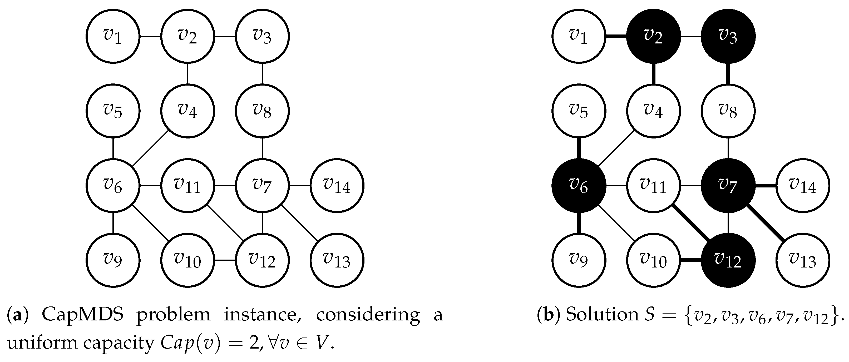
Cmsa++ for the CapMDS problem is provided in Algorithm 1. The algorithm maintains, at all times, an initially empty subset V of the set of vertices V of the input graph. This set is henceforth called the sub-instance. Vertices are added to sub-instance V by means of a probabilistic solution construction process, which is implemented in function ProbabilisticSolutionGeneration ( d rate , l size , g opt ) (see line 10 of Algorithm 1). In particular, all dominator vertices found in the solutions generated by this function are added to V —if not already in V —and their so-called “age value” age [ ] is initialized to zero (see lines 12 and 13 of Algorithm 1). Moreover, solving the sub-instance V refers to the application of the ILP solver CPLEX in order to find—if possible within the imposed time limit of t solver seconds—the optimal solution to sub-instance V ; that is, the optimal CapMDS solution in G that is limited to only contain dominators from V . This is achieved by adding the following set of constraints to the ILP model from the previous section:
x i = 0 x i V \ V
The process of solving the sub-instance V is done in function ApplyExactSolver( V , t solver ); see line 16 of Algorithm 1.
Algorithm 1Cmsa++ for the CapMDS problem
 1: input: a problem instance ( G , C a p )
 2: input: values for age max , n a , t solver , l size (original CMSA parameters)
 3: input: values for d rate L , d rate U , A type , g opt (additional parameters)
 4:  S bsf : =
 5:  V
 6:  age [ v ] : = 0 for all v V
 7: while CPU time limit not reached do
 8:   d rate : = DeterminismAdjustment ( d rate L , d rate U )
 9:  for i = 1 , , n a do
10:    S ProbabilisticSolutionGeneration ( d rate , l size , g opt )
11:   for all v S and v V do
12:     age [ v ] : = 0
13:     V V { v }
14:   end for
15:  end for
16:   S opt ApplyExactSolver( V , t solver )
17:  if f ( S opt ) < f ( S bsf ) then S bsf S opt
18:  Adapt( V , S opt , age max , A type )
19: end while
20: output: S bsf
The algorithm takes as input the tackled problem instance ( G , C a p ) , and values for eight required parameters. The first four of them—see line 2 of Algorithm 1—are inherited from the original CMSA proposal, while the remaining four parameters—see line 3 of Algorithm 1—are in the context of the extensions that lead to Cmsa++. The eight parameters can be described as follows:
  • age max : establishes the number of iterations that a vertex is allowed to form part of sub-instance V without forming part of the solution to V returned by the ILP solver ( S opt ).
  • n a : defines the number of solutions generated in the construction phase of the algorithm at each iteration; that is, the number of calls to function ProbabilisticSolutionGeneration().
  • t solver : establishes the time limit (in seconds) used for running the ILP solver at each iteration.
  • l size , d rate L , d rate U : these three parameters determine the greediness of the solution construction process in function ProbabilisticSolutionGeneration(), which we described in more detail in the following subsection.
  • g opt : indicates the variant of the solution construction process.
  • A type : chooses between two different behaviors implemented for the sub-instance maintenance mechanism implemented in function Adapt().
As mentioned above, Cmsa++ is—like any CMSA algorithm—equipped with a sub-instance maintenance mechanism for discarding seemingly useless solution components from the sub-instance V at each iteration. The original implementation of this mechanism works as follows. First, the age values of all vertices in V are incremented. Second, the age values of all vertices in S opt are re-initialized to zero. Third, the vertices with age values greater than age max are erased from V . In particular, this original implementation is used in case A type = 0 . In the other case—that is, when A type = 1 —a probability age [ v ] / age max for being removed from V is assigned to each vertex v V with age max > 0 . Note that these probabilities linearly increase until reaching probability 1 for all vertices with an age value greater than age max . Both mechanisms are implemented in function Adapt( V , S opt , age max , A type ) (see line 18 of Algorithm 1). Their aim is to maintain V small enough in order to be able to solve the sub-instance (if possible) optimally. If this is not possible in the allotted computation time, the output S opt of function ApplyExactSolver( V , t solver ) is simply the best solution found by CPLEX within the given time.
One of the new features of Cmsa++ (in comparison to the original version from [11]) is a dynamic mechanism for adjusting the determinism rate ( d rate ) used during the solution construction at each iteration. The mechanism is the same as that described in [32]. In the original CMSA, this determinism rate was a fixed value between 0 and 1, determined by algorithm tuning. In contrast, Cmsa++ chooses a value for d rate at each iteration in function DeterminismAdjustment ( d rate L , d rate U ) from the interval [ d rate L , d rate U ] where 0 d rate L d rate U 1 . This is done under the hypothesis that Cmsa++ can escape from local optima, increasing the randomness of the algorithm. Whenever an iteration improves S bsf , the value of d rate is set back to its upper bound ( d rate U ) . Otherwise, the value of d rate is decreased by a factor determined by subtracting the lower bound vale from the upper bound value ( d rate U ) and dividing the result by 3.0. Finally, whenever the value of d rate falls below the lower bound, it is set back to the upper bound value. Adequate values for d rate L and d rate U must be determined by algorithm tuning. Note that the behavior of the original CMSA algorithm is obtained by setting d rate U = d rate L .
Finally, note that Cmsa++ iterates while a predefined CPU time limit is not reached. Moreover, it provides the best solution found during the search, S bsf , as output.

Probabilistic Solution Generation

The function used for generating solutions in a probabilistic way (in line 10 of Algorithm 1) is presented in Algorithm 2. Note that there are three ways of generating solutions that are pseudo-coded in this algorithm. They are indicated in terms of three options: opt 1 , opt 2 , and  opt 3 . Line 18 of Algorithm 2, for example, is only executed for options opt 1 and opt 3 . Note that option opt 1 implements the solution construction mechanism of the original CMSA algorithm for the CapMDS problem from [11]. In the following section, first, the general solution construction procedure is described. Subsequently, we outline the differences between the three options mentioned above.
Algorithm 2 Function ProbabilisticSolutionGeneration( d rate , l size , g opt )
 1: input: a problem instance ( G , C a p )
 2: input: parameter values for l size , d rate , g opt
 3:  S : =
 4:  W : = V
 5:  V uncov : = V
 6: ComputeHeuristicValues(W)
 7: while V uncov do
 8:  Choose a random number δ [ 0 , 1 ]
 9:  if δ d rate then
10:   Choose v V such as h ( v ) h ( v ) for all v W
11:  else
12:   Let L W contain the min { l size , | W | } vertices from W with the highest heuristic values
13:   Choose v uniformly at random from L
14:  end if
15:   S : = S { v }
16:   V uncov : = V uncov \ ( C ( v ) { v } )
17:  if g opt = opt 1 or g opt = opt 3 then
18:    W : = W \ ( C ( v ) { v } )
19:  else
20:    W : = W \ { v }
21:  end if
22:  if g opt = opt 1 or g opt = opt 2 then
23:   ComputeHeuristicValues(W)
24:  end if
25: end while
26: output: S
The procedure takes as input the problem instance ( G , C a p ) , as well as values for the parameters l size , d rate and g opt . The two first parameters are used for controlling the degree of determinism of the solution construction process. Meanwhile, g opt indicates one of the three options. The process starts with an empty partial solution S : = . At each step, exactly one vertex from a set W V is added to S, until the set of uncovered vertices ( V uncov ) is empty. Note that both W and V uncov are initially set to V. Next we explain how to choose a vertex v from W at each step of the procedure. First of all, vertices from W are evaluated in function ComputeHeuristicValues(W) by a dynamic greedy function h ( ) , which depends on the current partial solution S. More specifically:
h ( v ) : = 1 + min { C a p ( v ) , deg S ( v ) } v W
Hereby, C a p ( v ) refers to the capacity of v and deg S ( v ) : = | N uncov ( v ) | , where  N uncov ( v ) : = N ( v ) V uncov is the set of currently uncovered neighbors of v. The  h ( ) -value of a vertex is henceforth called its heuristic value. The choice of a vertex v is then done as follows. First, a value δ [ 0 , 1 ] is chosen uniformly at random. In case δ d rate , v is chosen as the vertex that has the highest heuristic value among all vertices in W. Otherwise, a candidate list L containing the min { l size , | W | } vertices from W with the highest heuristic values is generated, and  v is chosen from L uniformly at random. Thus, the greediness of the solution construction procedure depends on the values of the determinism rate ( d rate ) and the candidate list size ( l size ). Note that, when deg S ( v ) is greater than C a p ( v ) , we have to choose which vertices from the N ( v ) V uncov vertex v is going to cover. In our current implementation, the set of C a p ( v ) vertices is simply chosen from N ( v ) V uncov uniformly at random and stored in C ( v ) . Finally, W and V uncov are updated at the end of each step.
When g opt = opt 1 , the solution construction procedure is the same as that used in the original CMSA algorithm for the CapMDS problem. In particular, W is updated after each choice of a vertex v in line 18 by removing the newly covered vertices. This concerns the chosen vertex v and the vertices from C ( v ) that were chosen to be covered by v . Moreover, the greedy function values are always updated according to the current partial solution S (see line 23 of Algorithm 2). In contrast, when  g opt = opt 2 the update of W (see line 20) is done by only removing the chosen vertex v 
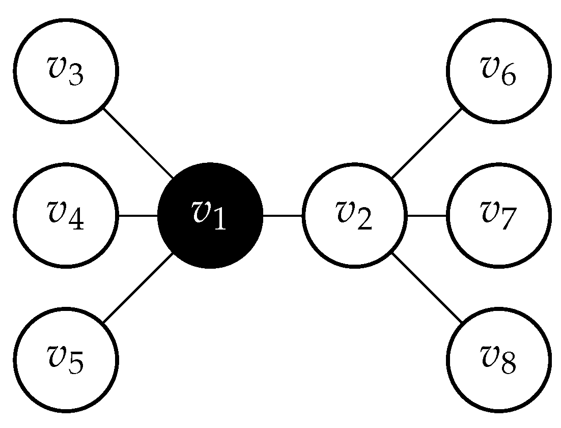
from the options. The rationale behind this is as follows. Consider the example in Figure 3. In case g opt = opt 1 , nodes v 1 and C v 1 = { v 2 , v 3 , v 4 , v 5 } are removed from W for the next construction step. This removes node v 2 from the set of selectable vertices, although choosing v 2 in the next step would lead to the construction of the optimal solution in this example.
Finally, with  g opt = opt 3 the solution construction is the same as with g opt = opt 1 , just that the greedy function values are not recalculated in line 23. The rationale behind this way of constructing solutions is to gain speed. On the negative side, this proposal possibly overestimates the heuristic values of the vertices and generally favors the hubs (vertices with a high degree) in the input graph.

3.2. Barrakuda: A Hybrid of Brkga with an ILp Solver

As mentioned before, the main algorithm proposed in this work is a hybrid between the well-known biased random key genetic algorithm (BRKGA) [31] and an ILP solver. Roughly, the solution components of (some of the solutions in the) population of the BRKGA are joined at the end of each iteration and the resulting sub-instance is passed to the ILP solver. Afterwards, the solution returned by the ILP solver is fed back into the population of BRKGA. As in CMSA, the main motivation for this proposal is to take profit from the ILP solver even in the context of problem instances that are too large in order to apply the ILP solver directly. The advantage of Barrakuda over CMSA is the learning component of BRKGA, which is not present in CMSA.

3.2.1. Main Algorithmic Framework

The main algorithm framework of Barrakuda, which is pseudo-coded in Algorithm 3, is that of the BRKGA. In fact, the lines that turn the BRKGA into Barrakuda are lines 12–15, which are marked by a different background colors. In the following section, we first outline all the BRKGA components of our algorithm before describing the additional Barrakuda components.
BRKGA is a steady-state genetic algorithm which consists of a problem-independent part and of a problem-dependent part. It takes as input the tackled problem instance ( G , C a p ) , and the values of four parameters ( p size , p e , p m and p r o b elite ) that are found in any BRKGA. The algorithm starts with the initialization of a population P composed of p size random individuals (line 4 of Algorithm 3). Each individual π P is a vector of length established by 2 | V | , where V is the set of vertices of G. In order to generate a random individual, for each position π ( i ) of π ( i = 1 , , 2 | V | ) a random value from [ 0 , 1 ] is generated. In this context, note that values π ( i ) and π ( i + | V | ) are associated to vertex v i of the input graph G. Then, the elements of the population are evaluated (see line 5 of Algorithm 3). This operation, which translates each individual π P into a solution S π (set of vertices) to the CapMDS problem, corresponds to the problem-dependent part described in the next subsection. Note that, after evaluation, each individual π P has assigned the objective function value f ( S π ) of corresponding CapMDS solution. Henceforth, f ( π ) will refer to f ( S π ) and vice versa.
Algorithm 3Barrakuda for the CapMDS problem
 1: input: a problem instance ( G , C a p )
 2: input: values for p size , p e , p m and p r o b elite (BRKGA parameters)
 3: input: values for n a , e x mode , t solver (additional Barrakuda parameters)
 4:  P GenerateInitialPopulation ( p size )
 5:  Evaluate ( P )
 6: while computation time limit not reached do
 7:   P e EliteSolutions ( P , p e )
 8:   P m Mutants ( P , p m )
 9:   P c Crossover ( P , P e , p r o b elite )
10:   Evaluate ( P m P c ) ▹ NOTE:  P e is already evaluated
11:   P : = P e P m P c
12:   P ilp ChooseSolutions ( P , e x mode , n a )
13:   V : = S P ilp S
14:   S opt ApplyExactSolver ( V , t solver )
15:   P IntegrateSolverSolution ( P , S opt )
16: end while
17: output: Best solution in P
Then, at each iteration of the algorithm, a set of genetic operators are executed in order to produce the population of the next iteration (see lines 7–11 in Algorithm 3). First, the best max { p e · p size , 1 } individuals are copied from P to P e in function EliteSolutions ( P , p e ) . Then, a set of max { p m · p size , 1 } mutant individuals are generated and stored in P m . These mutants are produced in the same way as individuals from the initial population. Next, a set of p size | P e | | P m | individuals are produced by crossover in function Crossover ( P , P e , p r o b elite ) and stored in P c . Each such individual is generated as follows: First, an elite parent π 1 is chosen uniformly at random from P e . Then, a second parent π 2 is chosen uniformly at random from P \ P e . Finally, an offspring individual π off is produced on the basis of π 1 and π 2 and stored in P c . In the context of the crossover operator, value π off ( i ) is set to π 1 ( i ) with probability p r o b elite , and to π 2 ( i ) otherwise. After generating all new offspring in P m and P c , these new individuals are evaluated in line 10. A standard BRKGA operation would now end after assembling the population of the next iteration (line 11).

3.2.2. Evaluation of an Individual

The problem-dependent part of the BRKGA concerns the evaluation of an individual, which consists of translating the individual into a valid CapMDS solution and calculating its objective function value. For this purpose, the solution generation procedure from Algorithm 2 is applied with option g opt = opt 2 . The only difference is in the choice of vertex v W at each step (lines 8–14 of Algorithm 2), and the choice of the set of neighbors C ( v ) to be covered by v . Both aspects are outlined in the following section. Moreover, the resulting pseudo-code is shown in Algorithm 4.
Instead of choosing a vertex v W at each iteration of the solution construction process in a semi-probabilistic way as shown in lines 8–14 of Algorithm 2, the choice is done deterministically based on combining the greedy function value h ( v i ) with its first corresponding value in individual π ( i ) . (Remember that function h ( ) is defined in Equation (7).) More specifically,
v : = argmax { h ( v i ) · π ( i ) v i W }
Algorithm 4 Evaluation of an individual in Barrakuda
 1: input: an individual π
 2:  S π : =
 3:  W : = V
 4:  V uncov : = V
 5: ComputeHeuristicValues(W)
 6: while V uncov do
 7:   v : = argmax { h ( v i ) · π ( i ) v i W }
 8:   S π : = S π { v }
 9:   C ( v ) =
10:   N : = N uncov ( v )
11:   r : = min { | N uncov ( v ) | , C a p ( v ) }
12:  while | C ( v ) | < r and v i N s.t.  π ( i + | V | ) > 0 do
13:    v : = argmax { | N uncov ( v i ) | · π ( i + | V | ) v i N }
14:    C ( v ) : = C ( v ) { v }
15:    N : = N \ { v }
16:  end while
17:   V uncov : = V uncov \ ( C ( v ) { v } )
18:   W : = W \ { v }
19:  ComputeHeuristicValues(W)
20: end while
21: output: S
This is also shown in line 7 of Algorithm 4. In this way, the BRKGA algorithm will produce—over time—individuals with high values π ( i ) for vertices v i that should form part of a solution, and vice versa. The greedy function h ( ) is only important for providing an initial bias towards an area in the search space that presumably contains good solutions. Finally, note that the first | V | values of an individual (corresponding, in the given order, to vertices v 1 , , v n } ) are used for deciding which vertices are chosen for the solution.
As mentioned above, the second aspect that differs when comparing the evaluation of an individual with the construction of a solution in Algorithm 2 is the choice of the set of neighbors C ( v ) to be covered by v at each step. Remember that, in Algorithm 2, min { | N uncov | , C a p ( v ) } , vertices are randomly chosen from N uncov ( v ) and stored in C ( v ) . In contrast, for the evaluation of a solution, vertices are sequentially picked from N uncov ( v ) and added to C ( v ) until either min { | N uncov | , C a p ( v ) } vertices are picked or no further uncovered neighbor v i of v exists with π ( i + | V | ) > 0 . Assuming that we denote the set of remaining (still unpicked) uncovered vertices of v by N, at each step the following vertex is picked from N:
v : = argmax { | N uncov ( v i ) | · π ( i + | V | ) v i N }
This is also shown in line 13 of Algorithm 4. Note that, as a greedy function for choosing from the uncovered neighbors of v , we make use of the number of uncovered neighbors of these vertices, preferring those with a large number of uncovered neighbors. Note also that, for selecting the vertices that are dominated by a chosen node v , the second half of an individual is used, that is, values  π ( | V | + 1 ) , , π ( 2 | V | ) . In other words, with the second half of an individual, the BRKGA learns by which node a non-chosen node should be covered.

3.2.3. From Brkga to Barrakuda

Finally, it remains to describe lines 12–15 of Algorithm 3 that are an addition to the standard BRKGA algorithm and that convert the algorithm into Barrakuda. This part makes use of three Barrakuda-specific parameters:
  • Parameter t solver is used for establishing the time limit given to the ILP solver in function ApplyExactSolver ( V , t solver ) .
  • Parameter e x m o d e is used for determining the way in which individuals/solutions are chosen from the current BRKGA population for building a sub-instance V . This is done in function ChooseSolutions ( P , e x mode , n a ) .
  • Parameter n a refers to the number of individuals that must be chosen from P for the construction of the sub-instance.
The Barrakuda-specific part of the algorithm starts by choosing exactly n a < p size individuals from the current population P and storing their corresponding solutions (which are known, because these individuals are already evaluated) in a set P ilp . Parameter e x mode indicates the way in which these n a solutions are chosen. In case e x mode = ELITIST , the  n a best individuals from P are chosen. Otherwise (when e x mode = RANDOM ), the best individual from P in addition to ( n a 1 ) randomly chosen solutions are added to P ilp . Subsequently, the vertices of all solutions from P ilp are merged into set V , and CPLEX is applied in function ApplyExactSolver ( V , t solver ) in the same way as in the case of Cmsa++. Finally, the solution S opt returned by the solver is fed back to BRKGA in function IntegrateSolverSolution ( P , S opt ) . More specifically, S opt is transformed into an individual π , which is then added to P. Finally, the worst individual is deleted from P in order to keep the population size constant. The integration process is quite straightforward, because it only considers information about the vertices (dominators) used in the solvers’ solution and not the domination relationships (edges). More specifically, Barrakuda creates a new individual π where π ( i ) : = 0.5 , i { | V | + 1 , | V | + 2 , , 2 | V | } . Moreover, for each dominating vertex v i in the solution of the solver π ( i ) : = 1.0 , whereas for each remaining vertex v j , the value of π ( j ) , is set to zero.

4. Experimental Evaluation

In this section, we present the comparison of our two algorithmic proposals: Cmsa++ and Barrakuda. For this purpose, we employ four different sets of problem instances. Two of them were presented in [9] and previously used in [11]. The remaining two instance sets are newly generated, because we noticed that most of the existing problem instances from the first two data sets are too small—respectively, too easy to solve—in order to be challenging. All four benchmark sets will be described in the following subsection.
We implemented all algorithms from scratch using ANSI C++ and compiled the code with GCC 8.3.0 (Ubuntu/Linux). Moreover, IBM ILOG CPLEX Optimization Studio V12.8.0 was executed in one-threaded mode, both as a standalone application (henceforth simply called Cplex) and within Cmsa++ and Barrakuda for solving the generated sub-instances. All experiments were conducted on the computing cluster of the Engineering Faculty of the University of Concepción (Luthier). Luthier is composed of 30 computing nodes, which all have the same hardware and software configuration. In particular, all nodes have an Intel CPU Xeon E3-1270 v6 at 3.8 GHz with 64 GB RAM. The cluster uses SLURM v17.11.2 for management and job scheduling purposes. The time limit for all experiments was 1000 CPU seconds per algorithm and per run, for all problem instances.

4.1. Benchmark Instances

The first two benchmark sets were taken from the literature. They were initially presented in [9] and later used for the experimental evaluation of the current state-of-the-art method in [10]. The first benchmark set contains 120 unit disk graphs (UDGs) created using the topology generator from [33]. In these instances, the vertices of each graph are randomly distributed over a Euclidean square of size 1000 × 1000 . Moreover, the graphs are generated with two different range values: 150 and 200 units. Note that with a range value of 150, for example, an undirected edge is introduced between each pair of vertices whose Euclidean distance is mostly 150 units. Accordingly, graphs on the same number of vertices become more dense with a growing range value used for generating them. The second benchmark set consists of 180 general graphs taken from the set of so-called type I instances originally proposed by Shyu et al. [34] in the context of the minimum weight vertex cover problem. For each graph size (in terms of the number of vertices) this benchmark set contains graphs from three different densities as indicted by their number of undirected edges. In both benchmark sets, the number of vertices of the graphs is from { 50 , 100 , 250 , 500 , 800 , 1000 } . Finally, graphs with vertices of two types of capacities—namely uniform capacities and variable capacities—can be found in these benchmark sets. In the case of uniform capacity, three different capacities of 2, 5 and α are tested, where α is graph-specific and is taken as the average degree of the corresponding graph. In the case of variable capacities, the vertex capacities are randomly chosen from the following three intervals: ( 2 , 5 ) , ( α / 5 , α / 2 ) and [ 1 , α ] . Note that the instance files come with the capacities already explicitly assigned. Note that for each combination of graph size (number of vertices), density (as determined by range values, respectively, number of edges) and capacity type/range, the benchmark sets consist of 10 randomly generated problem instances.
As we had already noticed in our preliminary work [11] that many of the problem instances from the above-mentioned benchmark sets are easily solved by Cplex, we decided generate more challenging instances, as follow. The first set is composed of general random graphs with 1000 or 5000 nodes. In this set, the number of edges depends on a parameter called edge probability ( e p ). This parameter is used in the construction of the graphs, where each possible edge is generated with probability e p . The probabilities that we considered are from { 0.05 , 0.15 , 0.25 } . Finally, we chose to generate instances with a uniform capacity of α , and others with a variable capacity for each vertex randomly chosen from [ 1 , α ] . The second one of the new benchmark sets is composed of random geometric graphs that are generated in a similar way as the unit disc graph instances mentioned above. All vertices are randomly distributed over the euclidean square—that is, a square of size 1.0 × 1.0 —and a connection radius r determines the edges. In particular, all vertices whose Euclidean distance is at most r are connected by an edge. Note that the radius r determines the density of the resulting graph. We used radius values from { 0.14 , 0.24 , 0.34 } . For this set we also considered instances with 1000 and 5000 vertices, as well as uniform capacity graphs with capacity α assigned to each node and variable capacity problems with a random capacity from [ 1 , α ] assigned to each vertex. In both cases (general random graphs and random geometric graphs) we generated 10 instances for each combination of graph size, density, and capacity type/size.

4.2. Tuning Process

As mentioned before, the reason for introducing Cmsa++, which is an extension of the Cmsa algorithm presented in preliminary work [11], was that Cmsa was not robust at all. Its parameters had to be tuned separately for many sub-groups of the set of available benchmark instances. Only in this way, the algorithm obtained very good results. In order to confirm that Cmsa++ and Barrakuda are sufficiently robust algorithms, a significantly lower number of algorithm configurations than those produced in [11] for Cmsa are produced for the final evaluation of Cmsa++ and Barrakuda. In particular, we produce different algorithm configurations only for 12 subsets of the instances from the literature. This is in contrast to 36 configurations that were produced for Cmsa in [11]. Remember in this context that Cmsa++ is—from an algorithmic point of view—a superset of Cmsa. This means that, if the proposed extensions are not found to be useful, the tuning process would choose the parameter settings, such that Cmsa++ is the same as Cmsa.
As outlined in the previous section, Cmsa++ requires well-working parameter values for parameters { age max , n a , t solver , l size , d rate L , d rate U , A type , g opt }, while Barrakuda required values for parameters { p size , p e , p m , p r o b elite , n a , e x m o d e , t solver }. Please refer to Section 3 for a comprehensive description of their function. We employ the scientific parameter tuning tool irace [35] for determining the values of these parameters. The parameters’ value domains for all the tuning runs were chosen as follows.
Cmsa++ parameter domains:
  • age max : { 1 , 2 , 3 , 5 , 10 , 1000 }
  • n a : { 1 , 2 , 5 , 10 , 30 , 50 }
  • t solver : { 3 , 5 , 10 , 50 , 75 , 100 , 250 , 500 }
  • l size : { 3 , 5 , 10 , 20 , 50 , 100 }
  • d rate L : [ 0 , 0.9 ]
  • d rate U : [ 0 , 0.9 ]
  • A type : { 0 , 1 }
  • g opt : { 1 , 210 , 2 }
Barrakuda parameter domains:
  • p size : { 10 , 20 , 50 , 100 , 200 , 500 }
  • p e : { 0.1 , 0.15 , 0.2 , 0.25 }
  • p m : { 0.1 , 0.15 , 0.2 , 0.25 , 0.3 }
  • p r o b elite : [ 0.5 , 0.9 ]
  • n a : { 1 , 3 , 5 , 10 , 30 , 50 }
  • e x mode : { 0 , 1 }
  • t solver : { 3 , 5 , 10 , 50 , 75 , 100 , 200 , 500 }
Hereby, real-valued parameters, such as d rate L , for example, are all treated with a precision of two positions behind the comma—that is, parameter d rate L whose domain is [ 0 , 0.9 ] can take values from { 0.0 , 0.01 , , 0.89 , 0.9 } .
Table 1 and Table 2 show the parameter value configurations of Cmsa++ and Barrakuda for the problem instances from the literature. Note that we distinguish between small problem instances (marked by S in the first table columns) and large problem instances (marked by L). Hereby, configuration S is for all instances with { 50 , 100 , 250 } vertices, and configuration L for the remaining (large) problem instances. Moreover, tuning is performed for three different capacity types; see the second table columns. Parameter values from the rows with { 2 , ( 2 , 5 ) } in the second column are, for example, for all instances with a uniform capacity of 2, and for all instances with a variable capacity from ( 2 , 5 ) .
Table 3 and Table 4 show the parameter values determined by irace for the instances from the new data set of large random graphs (RGs) and large random geometric graphs (RGGs) for Cmsa++ and Barrakuda, respectively. In these cases, the tuning for the uniform capacity problems was done separately from the variable capacity problems.
Finally, note that the original BRKGA algorithm can be obtained from Barrakuda by a setting of n a = 1 , which means that the sub-instance V is built from only one solution and that the ILP solver can therefore not find any better solution in the sub-instance. In fact, the setting of n a = 1 was determined by irace very few times, such as, for example, for the instances of the first row in Table 2a. In other words, in these cases the original BRKGA algorithm is better than Barrakuda. In the overwhelming majority of the cases, however, Barrakuda is significantly better than BRKGA.

4.3. Results

In addition to Cplex, Cmsa++ and Barrakuda were applied with the corresponding parameter values from above to all problem instances exactly once. The time limit for each run was set to 1000 CPU seconds for each algorithm. The results for the problem instances from the literature are presented in numerical form in Table 5, Table 6, Table 7 and Table 8. Each table row contains the solution quality (columns with heading q ¯ ) and the time at which this result was obtained (columns with heading t ¯ ) averaged over 10 problem instances for each of the three algorithms. Moreover, we show the results of LS_PD, which is an algorithm based on a local search that was the state-of-the-art approach for the CapMDS problem before the publication of Cmsa. In addition to solution quality and computation time, in the case of Cmsa++ and Barrakuda we also provide the average gap (in percent) over the respective 10 problem instances, either with respect to the optimal solutions obtained by Cplex, or—if not possible—with respect to the optimal MDS solutions of the respective problem instances. In the former case, the gaps are marked by a superscript ‘’a”, and in the latter one by a superscript ‘’b”. Those cases in which not even the optimal MDS solutions could be computed (due to excessive computation times) are marked with ‘’– –”. The best results per table row are indicated in bold font. Moreover, the result of Cplex is shown with a grey background in case the result is proven optimal. Finally, results with a preceding asterisk indicate new best-known results. In order to summarize these results, we additionally generated so-called critical difference (CD) plots for subsets of these problem instances (see the graphics in Figure 4). For their generation, first, the Friedman test was used to compare Cplex, Cmsa++ and Barrakuda simultaneously. (LS_PD was not included in the critical difference plots because, unfortunately, the detailed results per instance were not available. In any case, LS_PD is clearly worse than the other three techniques.) The hypothesis that the techniques perform equally was rejected. Subsequently, the algorithms were compared pairwise by the Nemenyi post-hoc test [36]. The obtained results can graphically be shown in the form of the above-mentioned CD plots in which each algorithm is placed on the horizontal axis according to its average ranking for the considered subset of problem instances. The performances of those algorithm variants that are below the critical difference threshold (computed with a significance level of 0.05) are considered as statistically equivalent. Such cases are shown by additional horizontal bars joining the average ranking markers of the respective algorithm variants. (The statistical evaluation was conducted using R’s scmamp package [37], available at https://github.com/b0rxa/scmamp.)
The following observations can be made:
  • First of all, Cplex as well as Cmsa++ and Barrakuda clearly outperform LS_PD on most problem instances.
  • However, most of the instances from the literature are no challenge, neither for the exact solver (Cplex), nor for the heuristic solvers proposed in this work (Cmsa++ and Barrakuda). In fact, Cplex is able to solve most problem instances to optimality; see the cases with a grey background. Interestingly, Cplex seems to have more problems with unit disk graphs than with random graphs. Moreover, instances with variable node capacities seem slightly harder as well. This is also indicated by the CD plots in Figure 4b–g. In particular, the CD plots in Figure 4b,d,f show that Cplex is not significantly worse than the best-performing algorithm. In the case of medium capacities (Figure 4d) Cplex even ranks best on average. In contrast, Figure 4c,e,g show that Barrakuda is (apart from the case of medium capacities) significantly better than Cplex and Cmsa++.
  • Even though we can only detect rather small differences between the three best-performing algorithms, when considering all problem instances from the literature together, Barrakuda performs significantly better than Cplex, which—in turn—performs significantly better than Cmsa.
The numerical results for the large problem instances from the new benchmark set are provided in Table 9 and Table 10. Note that the results for uniform capacity instances are shown in sub-tables (a) and for variable capacity instances in subtables (b). Finally, the corresponding critical difference plots are shown in Figure 5. Most notably, Cplex is now clearly worse than Cmsa++ and Barrakuda. In fact, in most cases, Cplex can only find the trivial solutions which contain all nodes of the input graph. Moreover, it is interesting to note that Barrakuda clearly outperforms Cmsa++ in the case of the random graph instances (see Table 9 and Figure 5b), while both methods perform statistically equivalent in the case of the random geometric graphs (see Table 10 and Figure 5c). Finally, it also worth mentioning that the MDS-based lower bound could be computed for nearly all random geometric graphs—apart from the cases with 5000 nodes and a low number of edges (S)—while this was not possible in the case of the random graphs (due to excessive computation times). Note that when the gap (see column with heading ”gap (%)”) is equal to zero, the algorithm’s result is equal to the MDS-based lower bound, which means that the optimal solutions are obtained in this these cases.

5. Conclusions and Future Work

In this paper we dealt with an NP-hard variant of the family of dominating set problems—the so-called minimum capacitated dominating set problem. Two algorithms were proposed to tackle this problem. The first one is an extended version of construct, merge, solved and adapt, of which a preliminary version was already published [11]. The aim of our extensions was to make the algorithm more robust with respect to the parameter value settings. The second algorithm that was proposed is a hybrid between a biased random key genetic algorithm and an exact solver. This solver was labeled Barrakuda. The main idea of Barrakuda is to use, at each iteration, the current population of individuals in order to generate a sub-instance of the tackled problem instances. This sub-instance is then solved by the exact solver (CPLEX) and the resulting solution is transformed into an individual and fed back into the population. The experimental results showed that both algorithms clearly outperform LS_PD, the currently best approach from the literature in the context of already published benchmark instances. However, the results also showed that these instances are not really a challenge for our algorithms. Therefore, we generated a new set of larger and more challenging benchmark instances. Barrakuda clearly outperformed the extended version of construct, merge, solve and adapt, especially in the context of general random graphs. In contrast, the performance of the two algorithms was shown to be quite similar for random geometric graphs.
Concerning future work, we want to study the reasons why Barrakuda performs (in relation to construct, merge and adapt) much better for general random graphs, while this difference does not show for random geometric graphs. Moreover, we believe that Barrakuda-type algorithms—that is, hybrid algorithms that (1) take profit from an exact solver and (2) incorporate a learning component—can be very successful for other types of combinatorial optimization problems, and this is something that we would like to study.

Author Contributions

Both authors contributed equally in all aspects of this research. All authors have read and agreed to the published version of the manuscript.

Funding

This work was supported by project CI-SUSTAIN funded by the Spanish Ministry of Science and Innovation (PID2019-104156GB-I00).

Acknowledgments

We acknowledge administrative and technical support by the Spanish National Research Council (CSIC) and the Universidad de Concepción, Chile.

Conflicts of Interest

The authors declare no conflict of interest. The funders had no role in the design of the study; in the collection, analyses, or interpretation of data; in the writing of the manuscript, or in the decision to publish the results.

References

  1. Yu, J.Y.; Chong, P.H.J. A survey of clustering schemes for mobile ad hoc networks. IEEE Commun. Surv. Tutor. 2005, 7, 32–48. [Google Scholar] [CrossRef]
  2. Rajaraman, R. Topology control and routing in ad hoc networks: A survey. ACM SIGACT News 2002, 33, 60–73. [Google Scholar] [CrossRef]
  3. Moscibroda, T. Clustering. In Algorithms for Sensor and Ad Hoc Networks: Advanced Lectures; Wagner, D., Wattenhofer, R., Eds.; Springer: Berlin/Heidelberg, Germany, 2007; pp. 37–61. [Google Scholar]
  4. Garey, M.R.; Johnson, D.S. Computers and Intractability: A Guide to the Theory of NP-Completeness; W. H. Freeman & Co.: New York, NY, USA, 1979. [Google Scholar]
  5. Cygan, M.; Pilipczuk, M.; Wojtaszczyk, J.O. Capacitated Domination Faster Than O(2n). In Algorithm Theory-SWAT 2010; Lecture Notes in Computer Science; Kaplan, H., Ed.; Springer: Berlin/Heidelberg, Germany, 2010; pp. 74–80. [Google Scholar]
  6. Liedloff, M.; Todinca, I.; Villanger, Y. Solving Capacitated Dominating Set by Using Covering by Subsets and Maximum Matching. In Graph Theoretic Concepts in Computer Science; Lecture Notes in Computer Science Thilikos, D.M., Ed.; Springer: Berlin/Heidelberg, Germany, 2010; pp. 88–99. [Google Scholar]
  7. Kuhn, F.; Moscibroda, T. Distributed approximation of capacitated dominating sets. Theory Comput. Syst. 2010, 47, 811–836. [Google Scholar] [CrossRef]
  8. Potluri, A.; Singh, A. A Greedy Heuristic and Its Variants for Minimum Capacitated Dominating Set. In Contemporary Computing; Communications in Computer and Information Science; Parashar, M.E.T., Ed.; Springer: Berlin/Heidelberg, Germany, 2012; pp. 28–39. [Google Scholar]
  9. Potluri, A.; Singh, A. Metaheuristic algorithms for computing capacitated dominating set with uniform and variable capacities. Swarm Evol. Comput. 2013, 13, 22–33. [Google Scholar] [CrossRef]
  10. Li, R.; Hu, S.; Zhao, P.; Zhou, Y.; Yin, M. A novel local search algorithm for the minimum capacitated dominating set. J. Oper. Res. Soc. 2018, 69, 849–863. [Google Scholar] [CrossRef]
  11. Pinacho-Davidson, P.; Bouamama, S.; Blum, C. Application of CMSA to the Minimum Capacitated Dominating Set Problem. In Proceedings of the Genetic and Evolutionary Computation Conference; ACM: New York, NY, USA, 2019; pp. 321–328. [Google Scholar] [CrossRef] [Green Version]
  12. Li, R.; Hu, S.; Liu, H.; Li, R.; Ouyang, D.; Yin, M. Multi-Start Local Search Algorithm for the Minimum Connected Dominating Set Problems. Mathematics 2019, 7, 1173. [Google Scholar] [CrossRef] [Green Version]
  13. Li, B.; Zhang, X.; Cai, S.; Lin, J.; Wang, Y.; Blum, C. NuCDS: An Efficient Local Search Algorithm for Minimum Connected Dominating Set. In Proceedings of the Twenty-Ninth International Joint Conference on Artificial Intelligence IJCAI-20, Yokohama, Japan, 11–17 July 2020; Bessiere, C., Ed.; International Joint Conferences on Artificial Intelligence Organization: Irvine, CA, USA, 2020; pp. 1503–1510. [Google Scholar]
  14. Bouamama, S.; Blum, C.; Fages, J.G. An algorithm based on ant colony optimization for the minimum connected dominating set problem. Appl. Soft Comput. 2019, 80, 672–686. [Google Scholar] [CrossRef]
  15. Wang, Y.; Li, C.; Yin, M. A two phase removing algorithm for minimum independent dominating set problem. Appl. Soft Comput. 2020, 88, 105949. [Google Scholar] [CrossRef]
  16. Wang, Y.; Chen, J.; Sun, H.; Yin, M. A memetic algorithm for minimum independent dominating set problem. Neural Comput. Appl. 2018, 30, 2519–2529. [Google Scholar] [CrossRef]
  17. Wang, Y.; Pan, S.; Li, C.; Yin, M. A local search algorithm with reinforcement learning based repair procedure for minimum weight independent dominating set. Inf. Sci. 2020, 512, 533–548. [Google Scholar] [CrossRef]
  18. Zhou, Y.; Li, J.; Liu, Y.; Lv, S.; Lai, Y.; Wang, J. Improved Memetic Algorithm for Solving the Minimum Weight Vertex Independent Dominating Set. Mathematics 2020, 8, 1155. [Google Scholar] [CrossRef]
  19. Yuan, F.; Li, C.; Gao, X.; Yin, M.; Wang, Y. A novel hybrid algorithm for minimum total dominating set problem. Mathematics 2019, 7, 222. [Google Scholar] [CrossRef] [Green Version]
  20. Cornejo Acosta, J.A.; García Díaz, J.; Menchaca-Méndez, R.; Menchaca-Méndez, R. Solving the Capacitated Vertex K-Center Problem through the Minimum Capacitated Dominating Set Problem. Mathematics 2020, 8, 1551. [Google Scholar] [CrossRef]
  21. Conejo, A.J.; Castillo, E.; Minguez, R.; Garcia-Bertrand, R. Decomposition Techniques in Mathematical Programming: Engineering and Science Applications; Springer Science & Business Media: New York, NY, USA, 2006. [Google Scholar]
  22. Boschetti, M.A.; Maniezzo, V.; Roffilli, M.; Bolufé Röhler, A. Matheuristics: Optimization, Simulation and Control. In Proceedings of HM 2009—6th International Workshop on Hybrid Metaheuristics; Lecture Notes in Computer Science; Blesa, M.J., Blum, C., Di Gaspero, L., Roli, A., Sampels, M., Schaerf, A., Eds.; Springer: Berlin/Heidelberg, Germany, 2009; pp. 171–177. [Google Scholar]
  23. Pisinger, D.; Røpke, S. Large Neighborhood Search. In Handbook of Metaheuristics; International Series in Operations Research & Management Science; Gendreau, M., Potvin, J.Y., Eds.; Springer: New York, NY, USA, 2010; pp. 399–419. [Google Scholar]
  24. Ahuja, R.K.; Orlin, J.B.; Sharma, D. Very large-scale neighborhood search. Int. Trans. Oper. Res. 2000, 7, 301–317. [Google Scholar] [CrossRef]
  25. Schrimpf, G.; Schneider, J.; Stamm-Wilbrandt, H.; Dueck, G. Record breaking optimization results using the ruin and recreate principle. J. Comput. Phys. 2000, 159, 139–171. [Google Scholar] [CrossRef] [Green Version]
  26. Fischetti, M.; Lodi, A. Local branching. Math. Program. 2003, 98, 23–47. [Google Scholar] [CrossRef]
  27. Caserta, M.; Voß, S. A corridor method based hybrid algorithm for redundancy allocation. J. Heuristics 2016, 22, 405–429. [Google Scholar] [CrossRef]
  28. Lalla-Ruiz, E.; Voß, S. POPMUSIC as a matheuristic for the berth allocation problem. Ann. Math. Artif. Intell. 2016, 76, 173–189. [Google Scholar] [CrossRef]
  29. Blum, C.; Pinacho, P.; López-Ibánez, M.; Lozano, J.A. Construct, Merge, Solve & Adapt: A new general algorithm for combinatorial optimization. Comput. Oper. Res. 2016, 68, 75–88. [Google Scholar] [CrossRef]
  30. Blum, C.; Raidl, G.R. Hybrid Metaheuristics, Powerful Tools for Optimization; Springer International Publishing: Cham, Switzerland, 2016. [Google Scholar]
  31. Gonçalves, J.F.; Resende, M.G.C. Biased random-key genetic algorithms for combinatorial optimization. J. Heuristics 2011, 17, 487–525. [Google Scholar] [CrossRef]
  32. Blum, C.; Gambini Santos, H. Generic CP-Supported CMSA for Binary Integer Linear Programs. In Hybrid Metaheuristics; Blesa Aguilera, M.J., Blum, C., Gambini Santos, H., Pinacho-Davidson, P., Godoy del Campo, J., Eds.; Springer International Publishing: Cham, Switzerland, 2019; pp. 1–15. [Google Scholar]
  33. Mastrogiovanni, M. The Clustering Simulation Framework: A Simple Manual. 2007. Available online: https://www.researchgate.net/publication/265429652_The_Clustering_Simulation_Framework_A_Simple_Manual (accessed on 11 March 2020).
  34. Shyu, S.J.; Yin, P.Y.; Lin, B.M. An ant colony optimization algorithm for the minimum weight vertex cover problem. Ann. Oper. Res. 2004, 131, 283–304. [Google Scholar] [CrossRef]
  35. López-Ibánez, M.; Dubois-Lacoste, J.; Cáceres, L.P.; Birattari, M.; Stützle, T. The irace package: Iterated racing for automatic algorithm configuration. Oper. Res. Perspect. 2016, 3, 43–58. [Google Scholar] [CrossRef]
  36. García, S.; Herrera, F. An Extension on “Statistical Comparisons of Classifiers over Multiple Data Sets” for all Pairwise Comparisons. J. Mach. Learn. Res. 2008, 9, 2677–2694. [Google Scholar]
  37. Calvo, B.; Santafé, G. Scmamp: Statistical Comparison of Multiple Algorithms in Multiple Problems. R J. 2016, 8, 2073–4859. [Google Scholar] [CrossRef] [Green Version]
Figure 1. An example of the CapMDS problem. Note that the bold edges in (b) indicate the domination relations. Vertices v 1 and v 4 , for example, are dominated by vertex v 2 which forms part of the solution.
Mathematics 08 01858 g001
Figure 2. High-level overview of the two proposed hybrid algorithms.
Mathematics 08 01858 g002
Figure 3. Example problem instance after the first step of generating a solution. Let us assume that the capacity of each node is 4. Vertex v 1 was chosen in the first step. As the capacity of v 1 is 4, all its neighbors are placed in C ( v 1 ) and covered by v 1 .
Mathematics 08 01858 g003
Figure 4. Critical difference plots concerning the problem instances from the literature.
Mathematics 08 01858 g004
Figure 5. Critical difference plots concerning the challenging large problem instances.
Mathematics 08 01858 g005
Table 1. Cmsa++ parameter values generated by irace for the instances from the literature.
SizeCapacity d rate L d rate U l size age max n a t solver A type g opt
{ 2 , ( 2 , 5 ) } 0.60.95513110
S { 5 , ( α / 5 , α / 2 ) } 0.10.71021100010
{ α , [ 1 , α ] } 0.60.7101250010
{ 2 , ( 2 , 5 ) } 0.20.25052100110
L { 5 , ( α / 5 , α / 2 ) } 0.60.95031250010
{ α , [ 1 , α ] } 0.20.31035100110
(a) Settings for unit disk graphs.
SizeCapacity d rate L d rate U l size age max n a t solver A type g opt
{ 2 , ( 2 , 5 ) } 0.30.450105101210
S { 5 , ( α / 5 , α / 2 ) } 0.50.8203305012
{ α , [ 1 , α ] } 0.10.250103010012
{ 2 , ( 2 , 5 ) } 0.40.7315100110
L { 5 , ( α / 5 , α / 2 ) } 0.80.9335250010
{ α , [ 1 , α ] } 0.50.92015250010
(b) Settings for general graphs.
Table 2. Barrakuda parameter values generated by irace for the instances from the literature.
SizeCapacity p size p e p m prob elite n a ex mode t solver
{ 2 , ( 2 , 5 ) } 1000.250.150.81010
S { 5 , ( α / 5 , α / 2 ) } 1000.250.30.830010
{ α , [ 1 , α ] } 2000.20.150.910075
{ 2 , ( 2 , 5 ) } 8000.250.20.821100
L { 5 , ( α / 5 , α / 2 ) } 200.20.150.52150
{ α , [ 1 , α ] } 5000.10.150.610075
(a) Settings for unit disk graphs.
SizeCapacity p size p e p m prob elite n a ex mode t solver
{ 2 , ( 2 , 5 ) } 5000.150.250.6501200
S { 5 , ( α / 5 , α / 2 ) } 8000.20.150.730010
{ α , [ 1 , α ] } 2000.150.150.9300100
{ 2 , ( 2 , 5 ) } 2000.20.150.950075
L { 5 , ( α / 5 , α / 2 ) } 5000.20.150.6301200
{ α , [ 1 , α ] } 8000.150.150.830010
(b) Settings for general graphs.
Table 3. Cmsa++ parameter values generated by irace for the new data set of large problem instances.
Typen ep / r Capacity d rate L d rate U l size age max n a t solver A type g opt
e p = 0.05 α 0.190.732010175110
RG1000 e p = 0.15 α 0.430.7333175110
e p = 0.25 α 0.10.52201175110
e p = 0.05 α 0.730.78532500010
RG5000 e p = 0.15 α 0.320.66551250110
e p = 0.25 α 0.320.68332500010
e p = 0.05 [ 1 , α ] 0.470.6131000175110
RG1000 e p = 0.15 [ 1 , α ] 0.020.56321100110
e p = 0.25 [ 1 , α ] 0.10.761031100110
e p = 0.05 [ 1 , α ] 0.090.21310001500110
RG5000 e p = 0.15 [ 1 , α ] 0.210.54511500010
e p = 0.25 [ 1 , α ] 0.260.83102250110
r = 0.14 α 0.110.55100355110
RGG1000 r = 0.24 α 0.480.8133575010
r = 0.34 α 0.470.910325012
r = 0.14 α 0.70.781025500110
RGG5000 r = 0.24 α 0.460.581035250110
r = 0.34 α 0.150.89100210500010
r = 0.14 [ 1 , α ] 0.050.6100102500110
RGG1000 r = 0.24 [ 1 , α ] 0.120.621001012501210
r = 0.34 [ 1 , α ] 0.360.73510501002
r = 0.14 [ 1 , α ] 0.110.162052500110
RGG5000 r = 0.24 [ 1 , α ] 0.550.625035500110
r = 0.34 [ 1 , α ] 0.650.892010550012
Table 4. Barrakuda parameter values generated by irace for the new data set of large problem instances.
Typen ep / r Capacity p size p e p m rhoe n a f mode t solver
e p = 0.05 α 5000.150.150.81003
RG1000 e p = 0.15 α 5000.10.150.821100
e p = 0.25 α 500.10.250.69215
e p = 0.05 α 5000.20.30.95005
RG5000 e p = 0.15 α 200.10.20.711075
e p = 0.25 α 200.10.150.822175
e p = 0.05 [ 1 , α ] 5000.150.150.81505
RG1000 e p = 0.15 [ 1 , α ] 5000.10.10.5320100
e p = 0.25 [ 1 , α ] 1000.20.20.6410500
e p = 0.05 [ 1 , α ] 5000.20.10.650110
RG5000 e p = 0.15 [ 1 , α ] 500.150.20.91075
e p = 0.25 [ 1 , α ] 1000.150.30.6810100
r = 0.14 α 500.250.30.56301100
RGG1000 r = 0.24 α 5000.20.10.682175
r = 0.34 α 500.250.10.715010
r = 0.14 α 500.150.10.8430175
RGG5000 r = 0.24 α 500.150.150.68501100
r = 0.34 α 500.150.20.68300500
r = 0.14 [ 1 , α ] 500.250.20.6950075
RGG1000 r = 0.24 [ 1 , α ] 2000.250.250.67100500
r = 0.34 [ 1 , α ] 500.10.10.565075
r = 0.14 [ 1 , α ] 5000.150.20.5850500
RGG5000 r = 0.24 [ 1 , α ] 1000.10.10.71100500
r = 0.34 [ 1 , α ] 500.250.150.54100500
Table 5. Results for general graphs with uniform capacity.
CapacitynRangeCplexLS_PDCmas++Barrakuda
q ¯ t ¯ q ¯ t ¯ q ¯ t ¯ gap (%) q ¯ t ¯ gap (%)
10017.0<0.117.0<0.117.0<0.1 0.0 a 17.00.1 0.0 a
25025017.0<0.117.0<0.117.00.1 0.0 a 17.00.1 0.0 a
50017.00.117.0<0.117.00.1 0.0 a 17.00.2 0.0 a
10034.00.234.0<0.134.00.1 0.0 a 34.00.1 0.0 a
210025034.00.134.0<0.134.00.1 0.0 a 34.00.2 0.0 a
50034.00.134.0<0.134.00.1 0.0 a 34.00.2 0.0 a
25084.01.784.03.684.00.2 0.0 a 84.00.4 0.0 a
225050084.00.484.05.784.00.3 0.0 a 84.00.6 0.0 a
100084.00.684.010.084.00.3 0.0 a 84.00.8 0.0 a
500167.010.8168.6<0.1167.06.9 0.0 a 167.00.7 0.0 a
25001000167.01.7170.255.5167.00.8 0.0 a 167.01.2 0.0 a
2000167.01.7167.538.4167.00.8 0.0 a 167.01.3 0.0 a
1000267.02.7274.2160.9267.01.3 0.0 a 267.02.2 0.0 a
28002000267.03.4272.7127.1267.02.0 0.0 a 267.03.2 0.0 a
5000267.04.6267.844.4267.01.8 0.0 a 267.03.5 0.0 a
1000334.0145.8338.4136.5334.058.4 0.0 a 334.02.7 0.0 a
210005000334.05.7336.0126.0334.02.9 0.0 a 334.04.9 0.0 a
10,000334.012.6334.04.2334.03.0 0.0 a 334.07.1 0.0 a
Avg. 150.512.0151.964.8150.54.4 150.51.6
10011.90.111.9<0.111.9<0.1 0.0 a 11.90.1 0.0 a
5502509.00.29.0<0.19.00.1 0.0 a 9.0<0.1 0.0 a
5009.00.29.0<0.19.00.1 0.0 a 9.0<0.1 0.0 a
10033.6<0.133.60.233.6<0.1 0.0 a 33.60.1 0.0 a
510025020.00.920.35.920.30.3 1.5 a 20.00.5 0.0 a
50017.00.617.00.117.00.2 0.0 a 17.00.4 0.0 a
25083.30.283.511.683.38.0 0.0 a 83.30.5 0.0 a
525050057.89.759.946.058.50.1 1.7 a 57.912.0 0.2 a
100042.015.745.032.642.01.6 0.0 a 42.012.3 0.0 a
500167.00.9168.310.7167.0371.7 0.0 a 167.01.5 0.0 a
55001000114.9821.4121.580.5115.6258.9 0.8 b 115.4540.9 0.6 b
200084.1254.192.271.384.00.8– –84.0136.7– –
1000242.55.8253.2101.8250.48.6 3.3 a 242.510.2 0.0 a
58002000164.81000.0176.2223.6167.5616.7– –166.2161.6– –
5000134.069.3140.4131.6134.015.4 0.0 a 134.025.1 0.0 a
1000333.73.1338.775.7333.73.8 0.0 a 333.74.5 0.0 a
510005000167.0205.6181.0140.3167.018.0 0.0 a 167.072.0 0.0 a
10,000167.0149.7171.062.7167.050.7 0.0 a 167.054.6 0.0 a
Avg. 103.3149.3107.366.3103.975.3 103.457.4
10012.00.212.0<0.112.00.2 0.0 a 12.00.1 0.0 a
α 502506.00.56.00.16.00.1 0.0 a 6.00.1 0.0 a
5003.80.93.8<0.13.80.2 0.0 a 3.8<0.1 0.0 a
10034.00.234.0<0.134.0<0.1 0.0 a 34.0<0.1 0.0 a
α 10025020.01.020.25.920.20.3 1.0 a 20.10.3 0.5 a
50012.25.512.22.612.22.8 0.0 a 12.23.0 0.0 a
25084.02.184.02.185.20.1 1.4 a 84.00.2 0.0 a
α 25050058.330.661.717.858.421.5 0.2 a 58.328.5 0.0 a
100036.7999.837.941.136.6326.6 1.4 b 36.5215.3 1.1 b
500167.015.8168.432.3167.00.9 0.0 a 167.01.7 0.0 a
α 5001000116.2966.2126.459.0117.0628.5 2.0 b 116.395.6 1.4 b
200075.31000.078.6101.075.7553.5– –74.3244.3– –
1000267.03.6274.0120.8267.01.4 0.0 a 267.04.8 0.0 a
α 8002000164.91001.0178.1159.2167.1589.1– – 162.6265.4– –
500091.1993.692.2329.491.2575.2– – 89.6569.7– –
1000334.0131.7338.434.7334.05.9 0.0 a 334.06.8 0.0 a
α 10005000132.5951.3137.4352.2133.6758.5– –134.2711.1– –
10,00087.6993.981.3604.883.2610.6– – 80.7663.6– –
Avg. 94.6394.397.0103.594.7226.4 94.0156.1
Total avg. 116.1185.2118.878.2116.4102.0 116.071.7
Table 6. Results for general graphs with variable capacity.
CapacitynRangeCplexLS_PDCmas++Barrakuda
q ¯ t ¯ q ¯ t ¯ q ¯ t ¯ gap (%) q ¯ t ¯ gap (%)
10013.00.113.00.213.00.1 0.0 a 13.00.1 0.0 a
( 2 , 5 ) 502509.00.19.0<0.19.0<0.1 0.0 a 9.00.1 0.0 a
5009.00.19.0<0.19.0<0.1 0.0 a 9.0<0.1 0.0 a
10033.70.133.70.133.7<0.1 0.0 a 33.70.1 0.0 a
( 2 , 5 ) 10025021.90.722.38.921.90.3 0.0 a 21.90.3 0.0 a
50017.00.417.26.517.00.2 0.0 a 17.00.3 0.0 a
25083.70.783.76.683.70.1 0.0 a 83.70.4 0.0 a
( 2 , 5 ) 25050063.211.966.520.763.21.9 0.0 a 63.21.9 0.0 a
100043.7177.148.420.643.9124.0 21.9 b 43.759.1 21.4 b
500167.04.5168.260.4167.29.2 0.1 a 167.00.8 0.0 a
( 2 , 5 ) 5001000125.5702.0135.2104.5125.8272.4 9.7 b 125.5302.0 9.4 b
200088.2725.398.963.287.9570.4– – 87.1603.4– –
1000248.123.1261.7180.3259.523.0 4.6 a 248.118.8 0.0 a
( 2 , 5 ) 8002000181.21000.0199.1174.9*180.7641.5– – 179.2643.9– –
5000134.134.9144.5161.5134.19.1 0.0 a 134.111.2 0.0 a
1000333.831.0338.6139.9334.082.8 0.06 a 333.82.9 0.0 a
( 2 , 5 ) 10005000169.0123.7189.4175.7169.050.6 0.0 a 169.046.2 0.0 a
10,000167.094.8172.2207.2167.08.6 0.0 a 167.023.7 0.0 a
Avg. 106.0162.8111.783.2106.699.7 105.895.3
10017.7<0.117.70.417.7<0.1 0.0 a 17.70.1 0.0 a
( α / 5 , α / 2 ) 502509.00.19.00.29.0<0.1 0.0 a 9.00.1 0.0 a
5005.00.45.0<0.15.00.1 0.0 a 5.0<0.1 0.0 a
10050.0<0.150.00.150.0<0.1 0.0 a 50.00.1 0.0 a
( α / 5 , α / 2 ) 10025034.30.134.96.734.3<0.1 0.0 a 34.30.2 0.0 a
50017.00.417.36.417.00.2 0.0 a 17.00.3 0.0 a
250125.00.2125.08.9125.00.1 0.0 a 125.00.5 0.0 a
( α / 5 , α / 2 ) 25050086.80.491.419.386.80.2 0.0 a 86.80.7 0.0 a
100051.41.054.920.251.40.5 0.0 a 51.41.1 0.0 a
500250.00.8251.161.2250.00.4 0.0 a 250.01.3 0.0 a
( α / 5 , α / 2 ) 5001000172.91.4183.536.5172.90.7 0.0 a 172.91.6 0.0 a
2000101.35.7110.859.8101.33.8 0.0 a 101.33.0 0.0 a
1000400.02.1401.685.9400.00.9 0.0 a 400.03.2 0.0 a
( α / 5 , α / 2 ) 8002000273.43.1292.2107.6273.42.5 0.0 a 273.43.9 0.0 a
5000115.074.3127.0101.8115.074.3 0.0 a 115.045.4 0.0 a
1000500.03.0505.6108.9500.01.4 0.0 a 500.05.0 0.0 a
( α / 5 , α / 2 ) 10005000168.1131.6188.0118.4168.159.5 0.0 a 168.139.3 0.0 a
10,000105.7841.6104.7123.0 102.0254.6– –109.8630.9– –
Avg. 137.966.6142.850.9137.722.2 138.240.9
10013.70.113.70.814.9<0.1 8.8 a 13.70.1 0.0 a
[ 1 , α ] 502507.20.47.20.68.4<0.1 16.7 a 7.20.1 0.0 a
5003.91.23.9<0.14.1<0.1 5.1 a 3.9<0.1 0.0 a
10040.10.140.1<0.140.1<0.1 0.0 a 40.1<0.1 0.0 a
[ 1 , α ] 10025023.30.723.77.426.4<0.1 13.3 a 23.30.2 0.0 a
50013.55.714.15.915.70.2 16.3 a 13.51.9 0.0 a
25098.90.399.06.698.90.1 0.0 a 98.90.2 0.0 a
[ 1 , α ] 25050067.33.471.518.772.10.2 7.1 a 67.31.0 0.0 a
100040.5948.844.627.346.82.2 30.0 b 40.3376.2 11.9 b
500202.70.9203.228.3202.70.6 0.0 a 202.71.8 0.0 a
[ 1 , α ] 5001000135.951.8147.755.0137.892.8 1.4 a 136.025.1 0.07 a
200083.11000.092.699.883.5527.2– –81.8164.1– –
1000300.22.1310.590.1300.22.2 0.0 a 300.24.6 0.0 a
[ 1 , α ] 8002000186.61000.0208.2124.8190.2554.6– – 185.8163.6– –
5000100.3985.7104.8227.2101.6608.0– – 97.3590.1– –
1000400.83.6405.0146.0400.83.5 0.0 a 400.86.8 0.0 a
[ 1 , α ] 10005000149.5949.9156.4335.5147.3730.8– – 142.7619.9– –
10,000132.91000.092.4387.091.6644.9– – 85.6670.4– –
Avg. 111.1330.8113.386.7110.2176.0 107.8145.9
Total avg. 118.4186.8122.673.6118.299.3 117.394.0
Table 7. Results for Unit Disk Graphs with uniform capacity.
CapacitynRangeCplexLS_PDCmas++Barrakuda
q ¯ t ¯ q ¯ t ¯ q ¯ t ¯ gap (%) q ¯ t ¯ gap (%)
25015017.2<0.117.20.117.20.1 0.0 a 17.21.8 0.0 a
25020017.00.117.0<0.117.0<0.1 0.0 a 17.0<0.1 0.0 a
210015034.00.134.50.134.00.1 0.0 a 34.00.1 0.0 a
210020034.00.234.1<0.134.0<0.1 0.0 a 34.00.1 0.0 a
225015084.00.886.0<0.184.00.2 0.0 a 84.00.3 0.0 a
225020084.00.985.4<0.184.00.2 0.0 a 84.00.4 0.0 a
2500150167.03.1171.60.2167.00.8 0.0 a 167.06.2 0.0 a
2500200167.04.4170.30.1167.00.9 0.0 a 167.012.1 0.0 a
2800150267.08.0273.90.2267.02.2 0.0 a 267.025.2 0.0 a
2800200267.011.7272.40.1267.02.2 0.0 a 267.046.3 0.0 a
21000150334.013.9342.6<0.1334.03.0 0.0 a 334.045.7 0.0 a
21000200334.019.1340.4<0.1334.03.7 0.0 a 334.082.4 0.0 a
Avg. 150.55.7153.80.1150.51.1 150.518.4
55015012.9<0.112.90.113.1<0.1 1.6 a 12.9<0.1 0.0 a
55020010.00.110.0<0.110.10.1 1.0 a 10.0<0.1 0.0 a
510015018.70.318.8<0.118.70.4 0.0 a 18.70.2 0.0 a
510020017.40.417.40.117.40.1 0.0 a 17.40.2 0.0 a
525015042.03.543.70.442.00.2 0.0 a 42.01.1 0.0 a
525020042.03.543.0<0.142.00.2 0.0 a 42.01.1 0.0 a
550015084.025.786.20.284.00.6 0.0 a 84.00.9 0.0 a
550020084.050.785.0<0.184.00.5 0.0 a 84.01.1 0.0 a
5800150134.0215.9137.01.0134.01.3 0.0 a 134.02.3 0.0 a
5800200134.0387.9135.70.1134.01.8 0.0 a 134.03.2 0.0 a
51000150167.0459.6171.02.7167.02.1 0.0 a 167.03.8 0.0 a
51000200173.3787.6169.6<0.1167.02.3– –167.05.3– –
Avg. 76.6175.977.50.776.10.8 76.11.6
α 5015014.4<0.114.479.414.4<0.1 0.0 a 14.4<0.1 0.0 a
α 5020010.00.110.022.510.1<0.1 1.0 a 10.0<0.1 0.0 a
α 10015018.70.318.9<0.118.70.3 0.0 a 18.70.2 0.0 a
α 10020011.00.411.0<0.111.00.1 0.0 a 11.00.2 0.0 a
α 25015018.54.519.48.318.52.9 0.0 a 18.61.5 0.5 a
α 25020011.36.311.51.711.32.0 0.0 a 11.40.9 0.9 a
α 50015018.6164.120.7250.118.772.3 0.5 a 19.114.2 2.7 a
α 50020011.390.912.1129.511.331.9 0.0 a 11.616.0 2.7 a
α 80015019.4906.221.3319.7 19.2239.2 1.6 b 19.480.7 2.1 b
α 80020012.3733.412.621.4 11.934.6 1.7 b 12.030.5 2.6 b
α 100015025.8942.421.52.6 19.4259.7 1.6 b 19.6143.0 2.6 b
α 100020014.7953.412.9<0.112.0104.9 0.0 b 12.099.1 0.0 b
Avg. 15.5345.615.592.814.762.3 14.832.2
Total avg. 80.9175.782.331.280.421.4 80.517.4
Table 8. Results for Unit Disk Graphs with variable capacity.
CapacitynRangeCplexLS_PDCmas++Barrakuda
q ¯ t ¯ q ¯ t ¯ q ¯ t ¯ gap (%) q ¯ t ¯ gap (%)
( 2 , 5 ) 5015014.5<0.114.5<0.114.9<0.1 2.8 a 14.50.4 0.0 a
( 2 , 5 ) 50200l11.10.111.1<0.111.2<0.1 0.9 a 11.10.1 0.0 a
( 2 , 5 ) 10015021.81.121.83.522.00.1 0.9 a 21.944.7 0.5 a
( 2 , 5 ) 10020017.60.417.83.717.60.9 0.0 a 17.60.3 0.0 a
( 2 , 5 ) 25015042.12.643.018.442.10.4 0.0 a 42.10.9 0.0 a
( 2 , 5 ) 25020042.02.342.036.042.00.2 0.0 a 42.00.3 0.0 a
( 2 , 5 ) 50015084.011.784.935.784.00.8 0.0 a 84.05.3 0.0 a
( 2 , 5 ) 50020084.015.284.033.484.00.8 0.0 a 84.09.6 0.0 a
( 2 , 5 ) 800150134.055.4134.9251.8134.01.7 0.0 a 134.020.5 0.0 a
( 2 , 5 ) 800200134.071.1134.1595.3134.02.0 0.0 a 134.040.0 0.0 a
( 2 , 5 ) 1000150167.0105.1168.6235.4167.02.9 0.0 a 167.037.2 0.0 a
( 2 , 5 ) 1000200167.0119.0167.5408.1167.03.3 0.0 a 167.070.6 0.0 a
Avg. 76.632.077.0135.176.71.1 76.619.2
( α / 5 , α / 2 ) 5015025.40.125.4<0.125.4<0.1 0.0 a 25.4<0.1 0.0 a
( α / 5 , α / 2 ) 5020017.3<0.117.30.117.3<0.1 0.0 a 17.3<0.1 0.0 a
( α / 5 , α / 2 ) 10015029.90.230.36.729.90.6 0.0 a 29.90.1 0.0 a
( α / 5 , α / 2 ) 10020017.80.417.83.417.80.1 0.0 a 17.80.1 0.0 a
( α / 5 , α / 2 ) 25015031.64.432.425.231.60.5 0.0 a 31.60.9 0.0 a
( α / 5 , α / 2 ) 25020018.926.319.213.318.90.5 0.0 a 18.93.6 0.0 a
( α / 5 , α / 2 ) 50015032.0661.532.935.932.02.5 0.0 a 32.02.4 0.0 a
( α / 5 , α / 2 ) 50020079.6602.319.4116.319.43.1 73.2 b 19.41.6 73.2 b
( α / 5 , α / 2 ) 800150732.0636.533.391.831.728.5 66.8 b 31.729.0 66.8 b
( α / 5 , α / 2 ) 800200796.61000.019.8100.119.64.7 67.5 b 19.64.6 67.5 b
( α / 5 , α / 2 ) 1000150997.81000.033.5173.632.513.3 70.2 b 32.57.2 70.2 b
( α / 5 , α / 2 ) 1000200996.01000.020.088.219.215.2 60.0 b 19.29.5 60.0 b
Avg. 314.6411.025.154.624.65.8 24.64.9
[ 1 , α ] 5015016.7<0.116.70.117.1<0.1 2.4 a 16.7<0.1 0.0 a
[ 1 , α ] 5020012.10.112.10.512.6<0.1 4.1 a 12.1<0.1 0.0 a
[ 1 , α ] 10015021.40.321.44.322.0<0.1 2.8 a 21.40.1 0.0 a
[ 1 , α ] 10020012.81.513.00.813.11.1 2.3 a 12.80.2 0.0 a
[ 1 , α ] 25015020.838.021.96.122.14.9 1.4 a 20.817.4 0.0 a
[ 1 , α ] 25020012.858.213.05.513.91.0 8.6 a 12.81.9 0.0 a
[ 1 , α ] 50015021.9940.622.655.722.812.2 18.9 b 21.1161.3 14.1 b
[ 1 , α ] 50020013.2926.113.053.013.511.6 20.5 b 12.731.5 13.4 b
[ 1 , α ] 80015022.7973.222.7163.023.0173.8 21.1 b 21.0324.4 10.5 b
[ 1 , α ] 800200726.9997.413.276.514.070.9 19.7 b 12.594.3 6.8 b
[ 1 , α ] 1000150909.21000.022.6500.422.5191.3 17.8 b 21.0495.9 9.9 b
[ 1 , α ] 10002001000.01000.013.0319.313.926.4 15.8 b 12.6162.8 5.0 b
Avg. 232.5494.617.198.817.541.1 16.5107.5
Total avg. 207.9312.539.796.139.616.0 39.243.9
Table 9. Experimental results for the random graphs from the new set of large problem instances.
Capacityn#EdgesCplexCmas++Barrakuda
q ¯ t ¯ g ¯ t ¯ q ¯ gap (%) q ¯ t ¯ gap (%)
S10001000.710048.3552.4– –46.1675.8– –
α 1000M10001000.810020.1392.2– –19.9302.8– –
L10001000.910012.9241.1– –12.9146.6– –
S50001018.210079.2227.7– –70.7777.4– –
α 5000M50001021.410031.1569.7– –28.4328.9– –
L50001024.810019.1167.6– –17.9190.6– –
Avg. 3000.01011.110035.1358.5 32.65403.7
(a) Uniform capacity problems.
Capacityn#EdgesCplexCmas++Barrakuda
q ¯ t ¯ g ¯ q ¯ t ¯ gap (%) q ¯ t ¯ gap (%)
S6030830.550.8565.4– –49.3690.3– –
[ 1 , α ] 1000M10001000.810020.5438.7– –20.0444.1– –
L1000100110012.9252.9– –12.8294.6– –
S50001018.210084.4481.2– –72.3700.0– –
[ 1 , α ] 5000M50001022.610031.8635.8– –28.8197.5– –
L50001025.610020.2236.5– –18.0171.6– –
Avg. 2843.3896.088.436.8435.1 33.5416.3
(b) Variable capacity problems.
Table 10. Experimental results for the random geometric graphs from the new set of large problem instances.
Capacityn#EdgesCplexCmas++Barrakuda
q ¯ t ¯ g ¯ q ¯ t ¯ gap (%) q ¯ t ¯ gap (%)
S22.7287.810.122.1200.3 0.9 b 22.2357.2 1.4 b
α 1000M10.6689.311.99.014.0 0.0 b 9.091.8 0.0 b
L10.1449.441.04.969.0 4.3 b 5.08.6 6.4 b
S4084.91018.810026.5720.3– –27.5736.3– –
α 5000M3926.01022.110010.0298.8 11.1 b 9.1690.3 1.1 b
L50001032.21005.2350.6 16.0 b 5.0477.1 0.0 b
Avg. 2175.7749.960.513.0275.5 13.0393.6
(a) Uniform capacity problems.
Capacityn#EdgesCplexCmas++Barrakuda
q ¯ t ¯ g ¯ q ¯ t ¯ gap (%) q ¯ t ¯ gap (%)
S26.7321.216.724.5225.6 12.4 b 24.5452.7 12.4 b
[ 1 , α ] 1000M334.5875.981.79.0120.6 0.0 b 9.055.3 0.0 b
L958.6951.91007.27.3 44.0 b 5.051.6 0.0 b
S50001018.210029.4646.6– –32.0818.5– –
[ 1 , α ] 5000M50001022.610010.5598.8 16.7 b 10.81229.9 20.0 b
L50001025.61005.8551.9 16.0 b 5.01138.2 0.0 b
Avg. 2720.0869.283.114.4358.5 14.4624.4
(b) Variable capacity problems.
Publisher’s Note: MDPI stays neutral with regard to jurisdictional claims in published maps and institutional affiliations.

