Hydrodynamical Study of Creeping Maxwell Fluid Flow through a Porous Slit with Uniform Reabsorption and Wall Slip

Abstract

The present theoretical study investigates the influence of velocity slip characteristics on the plane steady two-dimensional incompressible creeping Maxwell fluid flow passing through a porous slit with uniform reabsorption. This two-dimensional flow phenomenon is governed by the mathematical model having nonlinear partial differential equations together with non-homogeneous boundary conditions. An analytical technique, namely the recursive approach, is used successfully to find the solutions of the problem. The explicit expressions for stream function, velocity components, pressure distribution, wall shear stress and normal stress difference have been derived. The axial flow rate, leakage flux and fractional reabsorption are also found out. The points of maximum velocity are identified. Non-dimensionalization is carried out and graphs are portrayed at different positions of the channel to show the impact of pertinent parameters: slip parameter, Maxwell fluid parameter and absorption parameter, on flow variables and found that the fluid velocity is affected significantly due to these parameters. This study provides a mathematical basis to understand the physical phenomenon for fluid flows through permeable boundaries which exists in different problems like gaseous diffusion, filtration and biological mechanisms.

1. Introduction

Flow-through permeable boundaries have enormous importance from many decades due to their tremendous applications in bio-sciences and engineering, such as processes like membrane filtration, desalination processes using reverse osmosis, transpiration cooling, blood flow, renal proximal tubule flow within a kidney and filtration of blood in hemodialysis of an artificial kidney are the key examples related to flows in permeable boundaries [1,2,3,4,5,6]. Berman [7] presented the complete description of the Newtonian fluid flow through a channel with permeable walls and the perturbation method is employed to elaborate the wall permeability impact on velocity and pressure distribution. Sellars [8] and Yuan [9] extended this work to discuss the channel flow problem for high suction Reynolds number and for small and large seepage rates, respectively. Afterward, many researchers [10,11,12] further investigated the flow-through channel with permeable walls.

Due to the practical applications of creeping flow, many researchers studied the slow flow of Newtonian as well as non-Newtonian fluids. Macey [4] considered blood as an incompressible Newtonian fluid through the renal tubule and assumed creeping flow. Marshall [6] investigated the slow flow through a porous channel and discussed the obtained approximate solutions for ultrafiltration rate in flat plate hemodialyzer. Siddiqui and Haroon [13,14,15,16] considered different absorption rates on walls of the permeable slit to analyze the creeping flow of a Newtonian fluid. Rajagopal [17] considered the second order fluid to discuss the creeping flow. Ullah et al. [18,19] discussed the slow flow by considering the slightly viscoelastic fluid with uniform reabsorption using a recursive approach. Khashan et al. [20,21,22] also considered the creeping flow of micro-polar and Jeffrey fluids through a porous channel. Motivated with this, we have considered the Maxwell fluid to investigate the slow flow through permeable slit having wall slip with uniform reabsorption and present the solutions using the recursive approach proposed by Langlois [23,24].

For many decades, authors have been interested with slip condition due to its practical implications in the polymer industry (polymer melts) [25,26], which shows a macroscopic wall slip and also it extends from technological applications to medical applications as it used in polishing artificial heart valves. Beavers and Joseph [27] experimentally confirmed that the slip condition exists at the porous boundary. Saffman [28] gave the mathematical justification to the study presented by Beavers [27] and later, Beavers and Kohler [29,30] revealed that the already presented analytical results and their experimental outcomes are in good agreement. Mikelic and Jager [31] presented the statistical and mathematical analysis to discuss the slip above the porous surface. Rao et al. [32] discussed the slippage effects on viscous fluid flow in the channel. Elshahed [33] considered the velocity slip on membrane surface for blood flow in microcirculation. Singh et al. [34] showed the importance of velocity slip on ultra-filtration. Makinde and Osalusi [35] has explained the slip effects on the magnetohydrodynamic Newtonian fluid flow in a channel with porous walls. Eldesoky et al. [36] investigated the magnetohydrodynamics and slip effects on pulsatile blood flow through a porous medium having permeable walls and Elshehawy et al. [37] also discussed the velocity slip impact on peristaltic flow of Maxwellian fluid. Ellahi et al. [38] considered the channel flow of non-Newtonian fluid along with slip condition. Hron et al. [39] also considered the Naviers slip conditions at the boundary and discussed its impact on non-Newtonian fluids. Hayat et al. [40] discussed the Oldroyd 6-constant fluid flowing between parallel plates under the influenced of slip condition.

The significant importance of non-Newtonian fluid arises in plastic manufacturing, lubrication theory, paint industry and in food processing. Most of the biologically important fluids are considered as non-Newtonian due to their higher molecular weight. There are three categories of non-Newtonian fluids, namely: differential, rate and integral type fluids. The models of rate type fluids [41] has its importance and exhibits the stress relaxation aspects of polymer solutions. The expressions for stresses in terms of velocity components can be easily found out due to the existence of their explicit expressions in constitutive equations of differential type fluids, whether in the case of rate type fluids, there exits an implicit relationship in constitutive equation and its difficult to express stresses in terms of velocity components. This fact is the key reason for the lack of literature on the flow of rate type fluids through the permeable slit in the two dimensional case. To contribute with this, we consider the slow flow of Maxwell fluid in the two dimensional case through a permeable slit. An effort has been put by different researchers to investigate the flow of an upper convected Maxwell fluid. Choi et al. [42] investigated the combined effects of inertia, suction and viscoelasticity in a porous channel. Sadeghy et al. [43] studied Sakiadis flow and showed that wall skin friction decreases when increasing the value of Deborah’s number. Abbas et al. [44] also discussed the boundary layer magnetohydrodynamic Maxwell fluid flow in a permeable channel.

We consider the creeping flow of Maxwell fluid through the permeable slit in accordance with slip condition at porous walls and uniform reabsorption. The modeled nonlinear PDEs in accordance with non-homogeneous boundary conditions are solved with the recursive approach proposed by Langlois [23,24], who successfully implemented this approach for one-dimensional slow non-Newtonian fluid flows. Ullah et al. [18,19] used this technique for the first time to study two-dimensional creeping flow of a slightly viscoelastic fluid through a permeable slit. Recently, Bhatti et al. [45] used this approach to investigate the slow flow of a second order fluid through a uniformly permeable circular tube and now we implement this approach to get solutions of creeping flow of a Maxwell fluid and discuss combined effects of absorption parameter, viscoelasticity and slip parameter on flow variables involved at different positions of the channel and also obtain the explicit expressions for axial and radial velocity components, total pressure difference, mean pressure drop, normal stresses difference, wall shear stress, leakage flux and fractional reabsorption.

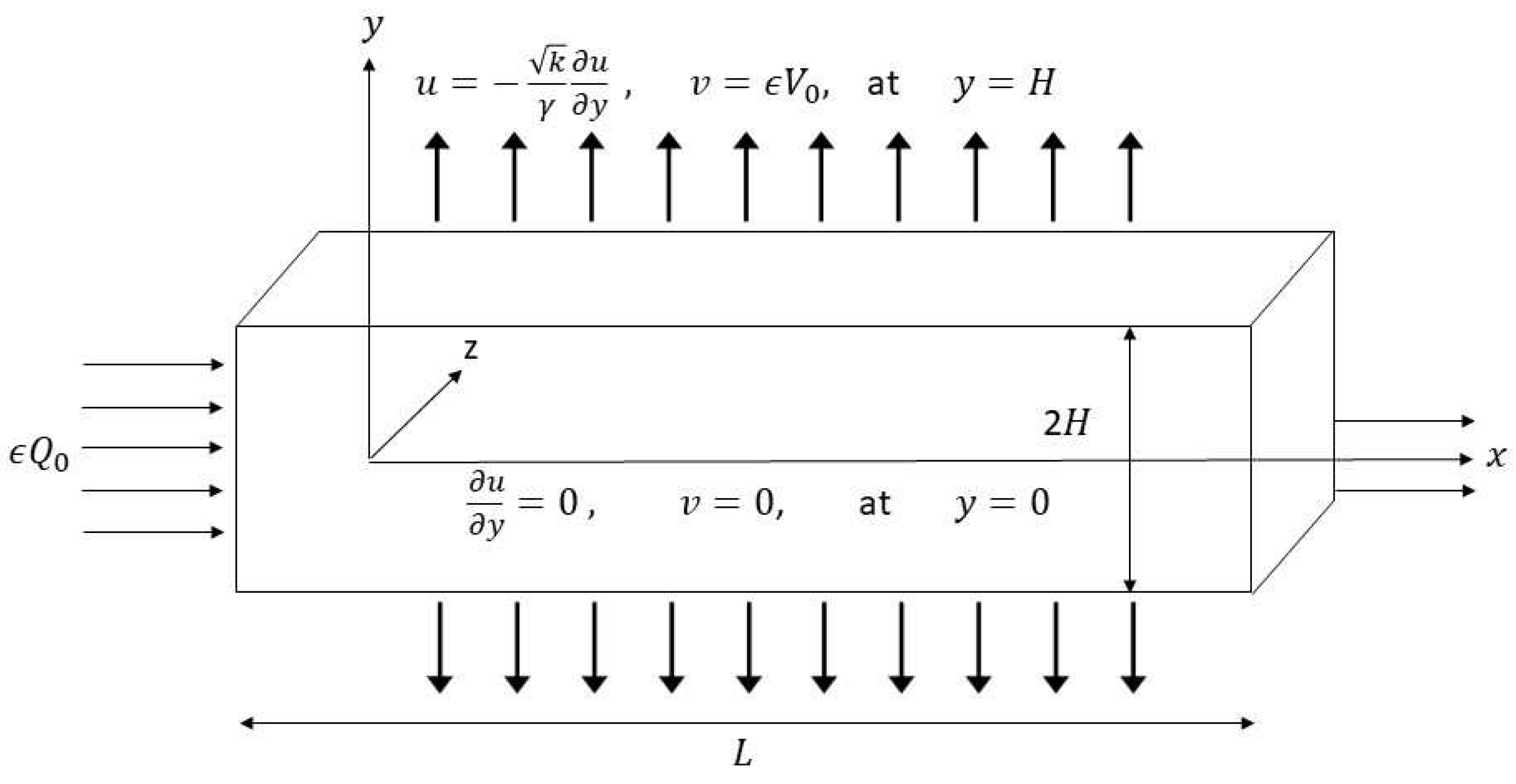
2. Formulation of the Problem

A two-dimensional isothermal, steady, incompressible creeping Maxwell fluid flow through a rectangular slit of length L, breadth W and width $2H$ is considered, with the x-axis taken along the centerline of the rectangular slit and y-axis taken normal to it. The walls of the slit are porous with a constant velocity of $ϵV_0$ along the slit length, where $ϵ$ is a small dimensionless parameter. A slip condition is also considered at porous walls of the slit and we assumed a constant flow rate $ϵQ_0$, at $x=0$, (see Figure 1).

In the proposed problem, the two-dimensional flow through the slit has the following velocity profile,

$$\begin{array}{c}\mathbf{V}=\left(u\right(x,y),v(x,y\left)\right)\hfill \end{array}$$

(1)

The conservation of mass and momentum equations for a creeping two-dimensional Maxwell fluid takes the form

$$\begin{array}{ccc}& & \frac{\partial u}{\partial x}+\frac{\partial v}{\partial y}=0,\hfill \end{array}$$

(2)

$$\begin{array}{ccc}& & \frac{\partial p}{\partial x}=\frac{\partial {\tau }_{xx}}{\partial x}+\frac{\partial {\tau }_{xy}}{\partial y},\hfill \end{array}$$

(3)

$$\begin{array}{ccc}& & \frac{\partial p}{\partial y}=\frac{\partial {\tau }_{xy}}{\partial x}+\frac{\partial {\tau }_{yy}}{\partial y},\hfill \end{array}$$

(4)

$$\begin{array}{ccc}& & {\tau }_{xx}+\lambda (u\frac{\partial {\tau }_{xx}}{\partial x}+v\frac{\partial {\tau }_{xx}}{\partial y}-2{\tau }_{xx}\frac{\partial u}{\partial x}-2{\tau }_{xy}\frac{\partial u}{\partial y})=2\mu \frac{\partial u}{\partial x},\hfill \end{array}$$

(5)

$$\begin{array}{ccc}& & {\tau }_{xy}+\lambda (u\frac{\partial {\tau }_{xy}}{\partial x}+v\frac{\partial {\tau }_{xy}}{\partial y}-{\tau }_{xx}\frac{\partial v}{\partial x}-{\tau }_{yy}\frac{\partial u}{\partial y})=\mu (\frac{\partial u}{\partial y}+\frac{\partial v}{\partial x}),\hfill \end{array}$$

(6)

$$\begin{array}{ccc}& & {\tau }_{yy}+\lambda (u\frac{\partial {\tau }_{yy}}{\partial x}+v\frac{\partial {\tau }_{yy}}{\partial y}-2{\tau }_{yy}\frac{\partial v}{\partial y}-2{\tau }_{xy}\frac{\partial v}{\partial x})=2\mu \frac{\partial v}{\partial y},\hfill \end{array}$$

(7)

where, (u, v) are axial and radial components of velocity, the constant $\lambda$ is the fluid relaxation time and $\mu$ is the viscosity of fluid. p and $\tau$ represent pressure and stresses of the Maxwell fluid, respectively.

The consequent boundary conditions are imposed as below by considering the upper half of the slit as due to symmetry along the centerline of the slit.

$$\begin{array}{ccc}& u=-{\displaystyle \frac{\sqrt{k}}{\gamma }}{\displaystyle \frac{\partial u}{\partial y}},v=ϵV_0,& \mathrm{at}y=H,\hfill \end{array}$$

(8)

$$\begin{array}{ccc}& {\displaystyle \frac{\partial u}{\partial y}}=0,v=0& \mathrm{at}y=0\hfill \end{array}$$

(9)

$$\begin{array}{cc}& ϵQ_0=W{\int }_{-H}^H\left(u(0,y)\right)dy.\end{array}$$

(10)

where k represents the specific permeability of a porous medium and $\gamma$ is a dimensionless constant. Here, the boundary condition (8) is the well-known slip condition given by Beavers and Joseph [27].

3. Solution of the Problem

The exact solution of the system of highly non-linear and coupled partial differential Equations (2)–(7) having six unknowns, namely, $u(x,y)$, $v(x,y)$, $p(x,y)$, ${\tau }_{xy}(x,y)$, ${\tau }_{xx}(x,y)$, ${\tau }_{yy}(x,y)$, together with non-homogeneous boundary conditions (8)–(10) is quite impossible and even analytical and numerical solutions of such equations are still a challenge for researchers. Here, we will use a recursive approach suggested by Langlois [23,24], which linearizes the above equations; so for this, we consider the flow field as a perturbation of a state of rest and the following is

$$\begin{array}{cc}& \mathbf{V}(x,y)={\sum }_{j=1}^{j=\infty }{ϵ}^j{\mathbf{V}}^{\left(j\right)}(x,y),\end{array}$$

(11)

$$\begin{array}{cc}& p(x,y)=Constant+{\sum }_{j=1}^{j=\infty }{ϵ}^j{p}^{\left(j\right)}(x,y),\end{array}$$

(12)

$$\begin{array}{cc}& \tau (x,y)={\sum }_{j=1}^{j=\infty }{ϵ}^j{\tau }^{\left(j\right)}(x,y).\end{array}$$

(13)

where $ϵ$ is a small dimensionless number.

The above supposition set up a dynamical system of linear equations and boundary conditions for each $[u^j,v^j,p^j,{\tau }^j]$, $j=1,2,3\dots$ and then $[u,v,p,\tau ]$ can be found by Equations (11)–(13), which will represent the solution for a creeping Maxwell fluid. The equations obtained for the first order $[u^1,v^1,p^1,{\tau }^1]$ are identical to the Newtonian fluid flow. The expressions obtained at the second order $[u^2,v^2,p^2,{\tau }^2]$ are similar with the exception that there exists non homogeneous terms depending on $[u^1,v^1,p^1,{\tau }^1]$. Likewise, $[u^3,v^3,p^3,{\tau }^3]$ are also similar but there also exits involvement of lower order solutions $[u^1,v^1,p^1,{\tau }^1]$, $[u^2,v^2,p^2,{\tau }^2]$ and this process continues recursively. It is also observed that a linear dynamical system of equations are formed at each stage of analysis and explicitly used results from previous stages. There is not too much practical or conceptual difficulty arising in extending the theory for higher orders.

In result of using Equations (11)–(13) into Equations (2)–(10) and comparing the coefficients of like powers of $ϵ$, we get three sets of systems of PDEs at $O\left(ϵ\right)$, $O\left({ϵ}^2\right)$ and $O\left({ϵ}^3\right)$.

3.1. System of Equations for the 1st Order

The first order system of equations is obtained by comparing coefficients of $ϵ$, as

$$\begin{array}{ccc}& & {\displaystyle \frac{\partial u^{\left(1\right)}}{\partial x}}+{\displaystyle \frac{\partial v^{\left(1\right)}}{\partial y}}=0,\hfill \end{array}$$

(14)

$$\begin{array}{ccc}& & {\displaystyle \frac{\partial p^{\left(1\right)}}{\partial x}}=\frac{\partial {\tau }_{xx}^{\left(1\right)}}{\partial x}+\frac{\partial {\tau }_{xy}^{\left(1\right)}}{\partial y},\hfill \end{array}$$

(15)

$$\begin{array}{ccc}& & {\displaystyle \frac{\partial p^{\left(1\right)}}{\partial y}}=\frac{\partial {\tau }_{xy}^{\left(1\right)}}{\partial x}+\frac{\partial {\tau }_{yy}^{\left(1\right)}}{\partial y},\hfill \end{array}$$

(16)

$$\begin{array}{ccc}& & {\tau }_{xx}^{\left(1\right)}=2\mu {\displaystyle \frac{\partial u^{\left(1\right)}}{\partial x}},{\tau }_{xy}^{\left(1\right)}=\mu \left({\displaystyle \frac{\partial u^{\left(1\right)}}{\partial y}}+{\displaystyle \frac{\partial v^{\left(1\right)}}{\partial x}}\right),{\tau }_{yy}^{\left(1\right)}=2\mu {\displaystyle \frac{\partial v^{\left(1\right)}}{\partial y}}.\hfill \end{array}$$

(17)

$$\begin{array}{ccc}& u^{\left(1\right)}=-{\displaystyle \frac{\sqrt{k}}{\gamma }}{\displaystyle \frac{\partial u^{\left(1\right)}}{\partial y}},v^{\left(1\right)}=V_0,& \mathrm{at}y=H,\hfill \end{array}$$

(18)

$$\begin{array}{ccc}& {\displaystyle \frac{\partial u^{\left(1\right)}}{\partial y}}=0,v^{\left(1\right)}=0,& \mathrm{at}y=0,\hfill \end{array}$$

(19)

$$\begin{array}{ccc}& {\int }_0^H(u^{\left(1\right)}(0,y))dy={\displaystyle \frac{Q_0}{2W}},& \mathrm{at}x=0.\hfill \end{array}$$

(20)

Here, we consider ${\psi }^{\left(1\right)}(x,y)$ as

$$u^{\left(1\right)}={\displaystyle \frac{\partial {\psi }^{\left(1\right)}(x,y)}{\partial y}},v^{\left(1\right)}=-{\displaystyle \frac{\partial {\psi }^{\left(1\right)}(x,y)}{\partial x}}.$$

(21)

We found that in view of Equation (21), Equation (14) is satisfied identically and after elimination of the pressure term, Equations (15), (16) and (18)–(20) in terms of $\psi (x,y)$ become,

$${\nabla }^4{\psi }^{\left(1\right)}=0.$$

(22)

$$\begin{array}{c}{\displaystyle \frac{\partial {\psi }^{\left(1\right)}}{\partial y}}=-{\displaystyle \frac{\sqrt{k}}{\gamma }}{\displaystyle \frac{{\partial }^2{\psi }^{\left(1\right)}}{\partial y^2}},{\displaystyle \frac{\partial {\psi }^{\left(1\right)}}{\partial x}}=-v_0,\mathrm{at}y=H,\hfill \end{array}$$

(23)

$$\begin{array}{c}{\displaystyle \frac{{\partial }^2{\psi }^{\left(1\right)}}{\partial y^2}}=0,{\displaystyle \frac{\partial {\psi }^{\left(1\right)}}{\partial x}}=0,\mathrm{at}y=0,\hfill \end{array}$$

(24)

$$\begin{array}{c}{\psi }^{\left(1\right)}(0,H)={\displaystyle \frac{Q_0}{2W}},{\psi }^{\left(1\right)}(0,0)=0.\hfill \end{array}$$

(25)

The boundary conditions (23)–(25) suggest to consider ${\psi }^{\left(1\right)}(x,y)$ as

$${\psi }^{\left(1\right)}(x,y)=V_{0}x{M}^{\left(1\right)}\left(y\right)+N^{\left(1\right)}\left(y\right).$$

(26)

where $M^{\left(1\right)}\left(y\right)$ and $N^{\left(1\right)}\left(y\right)$ are unknowns, which can be obtained by using Equation (26) in Equations (22)–(25) and ultimately we have

$$\begin{array}{ccc}{\mathrm{M}}^{\left(1\right)}\left(y\right)\hfill & =& \frac{1}{2}{b}_1\left(\frac{y^3}{H^3}-\frac{3b_{2}y}{H}\right),\hfill \end{array}$$

(27)

$$\begin{array}{ccc}{\mathrm{N}}^{\left(1\right)}\left(y\right)\hfill & =& \frac{\left(b_1{Q}_0\right)}{4W}\left(\frac{3b_{2}y}{H}-\frac{y^3}{H^3}\right).\hfill \end{array}$$

(28)

where $\varphi =\frac{\sqrt{k}}{H\gamma }$ is the slip parameter and $(b_1=\frac{1}{1+3\varphi })$ and $b_2=1+2\varphi$ are functions of $\varphi$.

Equation (26) in results of utilizing Equations (21), (27) and (28), we obtain

$$\begin{array}{ccc}{\psi }^{\left(1\right)}\hfill & =& \frac{b_1}{2}(\frac{Q_0}{2W}-x{V}_0)(\frac{3b_{2}y}{H}-\frac{y^3}{H^3}),\hfill \end{array}$$

(29)

$$\begin{array}{ccc}{u}^{\left(1\right)}\hfill & =& \frac{3b_1}{2H}(\frac{Q_0}{2W}-x{V}_0)(b_2-\frac{y^2}{H^2}),\hfill \end{array}$$

(30)

$$\begin{array}{ccc}{v}^{\left(1\right)}\hfill & =& \frac{b_1{V}_0}{2}(\frac{3b_{2}y}{H}-\frac{y^3}{H^3}),\hfill \end{array}$$

(31)

Here, we observed that the obtained first-order solution is strongly dependent on $\varphi$ and no contribution of Maxwell fluid parameter $\delta$ is found. It is observed that the expressions for velocity components at first order with $(\varphi =0)$ are similar to the results presented in [15].

3.2. System of Equations for the 2nd Order

On equating terms involving ${ϵ}^2$, we have the following system of equations:

$$\begin{array}{ccc}& & {\displaystyle \frac{\partial u^{\left(2\right)}}{\partial x}}+{\displaystyle \frac{\partial v^{\left(2\right)}}{\partial y}}=0,\hfill \end{array}$$

(32)

$$\begin{array}{ccc}& & {\displaystyle \frac{\partial p^{\left(2\right)}}{\partial x}}=\frac{\partial {\tau }_{xx}^{\left(2\right)}}{\partial x}+\frac{\partial {\tau }_{xy}^{\left(2\right)}}{\partial y},\hfill \end{array}$$

(33)

$$\begin{array}{ccc}& & {\displaystyle \frac{\partial p^{\left(2\right)}}{\partial y}}=\frac{\partial {\tau }_{xy}^{\left(2\right)}}{\partial x}+\frac{\partial {\tau }_{yy}^{\left(2\right)}}{\partial y},\hfill \end{array}$$

(34)

$$\begin{array}{ccc}& & {\tau }_{xx}^{\left(2\right)}+\lambda (u^{\left(1\right)}\frac{\partial {\tau }_{xx}^{\left(1\right)}}{\partial x}+v^{\left(1\right)}\frac{\partial {\tau }_{xx}^{\left(1\right)}}{\partial y}-2{\tau }_{xx}^{\left(1\right)}\frac{\partial u^{\left(1\right)}}{\partial x}-2{\tau }_{xy}^{\left(1\right)}\frac{\partial u^{\left(1\right)}}{\partial y})=2\mu \frac{\partial u^{\left(2\right)}}{\partial x},\hfill \end{array}$$

(35)

$$\begin{array}{ccc}& & {\tau }_{xy}^{\left(2\right)}+\lambda (u^{\left(1\right)}\frac{\partial {\tau }_{xy}^{\left(1\right)}}{\partial x}+v^{\left(1\right)}\frac{\partial {\tau }_{xy}^{\left(1\right)}}{\partial y}-{\tau }_{xx}^{\left(1\right)}\frac{\partial v^{\left(1\right)}}{\partial x}-{\tau }_{yy}^{\left(1\right)}\frac{\partial u^{\left(1\right)}}{\partial y})=\mu (\frac{\partial v^{\left(2\right)}}{\partial x}+\frac{\partial u^{\left(2\right)}}{\partial y}),\hfill \end{array}$$

(36)

$$\begin{array}{ccc}& & {\tau }_{yy}^{\left(2\right)}+\lambda (u^{\left(1\right)}\frac{\partial {\tau }_{yy}^{\left(1\right)}}{\partial x}+v^{\left(1\right)}\frac{\partial {\tau }_{yy}^{\left(1\right)}}{\partial y}-2{\tau }_{yy}^{\left(1\right)}\frac{\partial v^{\left(1\right)}}{\partial y}-2{\tau }_{xy}^{\left(1\right)}\frac{\partial v^{\left(1\right)}}{\partial x})=2\mu \frac{\partial v^{\left(2\right)}}{\partial y},\hfill \end{array}$$

(37)

$$\begin{array}{ccc}& u^{\left(2\right)}=-{\displaystyle \frac{\sqrt{k}}{\gamma }}{\displaystyle \frac{\partial u^{\left(2\right)}}{\partial y}},v^{\left(2\right)}=0,& \mathrm{at}y=H,\hfill \end{array}$$

(38)

$$\begin{array}{ccc}& {\displaystyle \frac{\partial u^{\left(2\right)}}{\partial y}}=0,v^{\left(2\right)}=0,& \mathrm{at}y=0,\hfill \end{array}$$

(39)

$$\begin{array}{ccc}& {\int }_0^H(u^{\left(2\right)}(0,y))dy=0,& \mathrm{at}x=0.\hfill \end{array}$$

(40)

We consider ${\psi }^{\left(2\right)}(x,y)$ as

$$u^{\left(2\right)}={\displaystyle \frac{\partial {\psi }^{\left(2\right)}(x,y)}{\partial y}},v^{\left(2\right)}=-{\displaystyle \frac{\partial {\psi }^{\left(2\right)}(x,y)}{\partial x}}.$$

(41)

Equation (32) is satisfied identically. Using the first order solution (29)–(31) in Equations (35)–(37) and then eliminating pressure from Equations (33) and (34), the resulting equation in terms of stream function becomes

$${\nabla }^4{\psi }^{\left(2\right)}=0,$$

(42)

The boundary conditions at this order take the following form

$$\begin{array}{ccc}& & {\displaystyle \frac{\partial {\psi }^{\left(2\right)}}{\partial y}}=-{\displaystyle \frac{\sqrt{k}}{\gamma }}{\displaystyle \frac{{\partial }^2{\psi }^{\left(2\right)}}{\partial y^2}},{\displaystyle \frac{\partial {\psi }^{\left(2\right)}}{\partial x}}=0,\mathrm{at}y=H,\hfill \end{array}$$

(43)

$$\begin{array}{ccc}& & {\displaystyle \frac{{\partial }^2{\psi }^{\left(2\right)}}{\partial y^2}}=0,{\displaystyle \frac{\partial {\psi }^{\left(2\right)}}{\partial x}}=0,\mathrm{at}y=0,\hfill \end{array}$$

(44)

$$\begin{array}{ccc}& & {\psi }^{\left(2\right)}(0,H)=0,{\psi }^{\left(2\right)}(0,0)=0.\hfill \end{array}$$

(45)

The solution of the system of Equations (42)–(45) becomes zero due to the homogeneous boundary conditions for any supposed form of ${\psi }^{\left(2\right)}(x,y)$. Therefore,

$$\begin{array}{ccc}{\psi }^{\left(2\right)}\hfill & =& 0,\hfill \end{array}$$

(46)

$$\begin{array}{ccc}{u}^{\left(2\right)}\hfill & =& 0,\hfill \end{array}$$

(47)

$$\begin{array}{ccc}{v}^{\left(2\right)}\hfill & =& 0,\hfill \end{array}$$

(48)

Thus, at this order, we do not see any contribution of Newtonian or viscoelastic effects towards the velocity field.

3.3. System of Equations for the 3rd Order

Equating terms involving ${ϵ}^3$ and the obtained system of equations along with boundary conditions are

$$\begin{array}{ccc}& & {\displaystyle \frac{\partial u^{\left(3\right)}}{\partial x}}+{\displaystyle \frac{\partial v^{\left(3\right)}}{\partial y}}=0,\hfill \end{array}$$

(49)

$$\begin{array}{ccc}& & {\displaystyle \frac{\partial p^{\left(3\right)}}{\partial x}}=\frac{\partial {\tau }_{xx}^{\left(3\right)}}{\partial x}+\frac{\partial {\tau }_{xy}^{\left(3\right)}}{\partial y},\hfill \end{array}$$

(50)

$$\begin{array}{ccc}& & {\displaystyle \frac{\partial p^{\left(3\right)}}{\partial y}}=\frac{\partial {\tau }_{xy}^{\left(3\right)}}{\partial x}+\frac{\partial {\tau }_{yy}^{\left(3\right)}}{\partial y},\hfill \end{array}$$

(51)

$$\begin{array}{ccc}& & {\tau }_{xx}^{\left(3\right)}+\lambda (u^{\left(1\right)}\frac{\partial {\tau }_{xx}^{\left(2\right)}}{\partial x}+v^{\left(1\right)}\frac{\partial {\tau }_{xx}^{\left(2\right)}}{\partial y}-2{\tau }_{xx}^{\left(2\right)}\frac{\partial u^{\left(1\right)}}{\partial x}-2{\tau }_{xy}^{\left(2\right)}\frac{\partial u^{\left(1\right)}}{\partial y}+u^{\left(2\right)}\frac{\partial {\tau }_{xx}^{\left(1\right)}}{\partial x}\hfill \\ & & +v^{\left(2\right)}\frac{\partial {\tau }_{xx}^{\left(1\right)}}{\partial y}-2{\tau }_{xx}^{\left(1\right)}\frac{\partial u^{\left(2\right)}}{\partial x}-2{\tau }_{xy}^{\left(1\right)}\frac{\partial u^{\left(2\right)}}{\partial y})=2\mu \frac{\partial u^{\left(3\right)}}{\partial x},\hfill \end{array}$$

(52)

$$\begin{array}{ccc}& & {\tau }_{xy}^{\left(3\right)}+\lambda (u^{\left(1\right)}\frac{\partial {\tau }_{xy}^{\left(2\right)}}{\partial x}+v^{\left(1\right)}\frac{\partial {\tau }_{xy}^{\left(2\right)}}{\partial y}-{\tau }_{xx}^{\left(2\right)}\frac{\partial v^{\left(1\right)}}{\partial x}-{\tau }_{yy}^{\left(2\right)}\frac{\partial u^{\left(1\right)}}{\partial y}+u^{\left(2\right)}\frac{\partial {\tau }_{xy}^{\left(1\right)}}{\partial x}\hfill \\ & & +v^{\left(2\right)}\frac{\partial {\tau }_{xy}^{\left(1\right)}}{\partial y}-{\tau }_{xx}^{\left(1\right)}\frac{\partial v^{\left(2\right)}}{\partial x}-{\tau }_{yy}^{\left(1\right)}\frac{\partial u^{\left(2\right)}}{\partial y})=\mu (\frac{\partial u^{\left(3\right)}}{\partial y}+\frac{\partial v^{\left(3\right)}}{\partial x}),\hfill \end{array}$$

(53)

$$\begin{array}{ccc}& & {\tau }_{yy}^{\left(3\right)}+\lambda (u^{\left(1\right)}\frac{\partial {\tau }_{yy}^{\left(2\right)}}{\partial x}+v^{\left(1\right)}\frac{\partial {\tau }_{yy}^{\left(2\right)}}{\partial y}-2{\tau }_{yy}^{\left(2\right)}\frac{\partial v^{\left(1\right)}}{\partial y}-2{\tau }_{xy}^{\left(2\right)}\frac{\partial v^{\left(1\right)}}{\partial x}+\frac{\partial {\tau }_{yy}^{\left(1\right)}}{\partial x}(u^{\left(2\right)})\hfill \\ & & +\frac{\partial {\tau }_{yy}^{\left(1\right)}}{\partial y}(v^{\left(2\right)})-2{\tau }_{yy}^{\left(1\right)}\frac{\partial v^{\left(2\right)}}{\partial y}-2{\tau }_{xy}^{\left(1\right)}\frac{\partial v^{\left(2\right)}}{\partial x})=2\mu \frac{\partial v^{\left(3\right)}}{\partial y},\hfill \end{array}$$

(54)

$$\begin{array}{ccc}& u^{\left(3\right)}=-{\displaystyle \frac{\sqrt{k}}{\gamma }}{\displaystyle \frac{\partial u^{\left(3\right)}}{\partial y}},v^{\left(3\right)}=0,& \mathrm{at}y=H,\hfill \end{array}$$

(55)

$$\begin{array}{ccc}& {\displaystyle \frac{\partial u^{\left(3\right)}}{\partial y}}=0,v^{\left(3\right)}=0,& \mathrm{at}y=0,\hfill \end{array}$$

(56)

$$\begin{array}{ccc}& {\int }_0^H(u^{\left(3\right)}(0,y))dy=0,& \mathrm{at}x=0.\hfill \end{array}$$

(57)

The ${\psi }^{\left(3\right)}(x,y)$ in the third order is define as

$$u^{\left(3\right)}={\displaystyle \frac{\partial {\psi }^{\left(3\right)}(x,y)}{\partial y}},v^{\left(3\right)}=-{\displaystyle \frac{\partial {\psi }^{\left(3\right)}(x,y)}{\partial x}}.$$

(58)

Equation (49) is satisfied identically. On substituting the first order solution (29)–(31) and the second order solution (46)–(48) along with Equation (58) into the third order system (53)–(55) and then eliminating the pressure by cross differentiation of Equations (50) and (51), we arrive at Equation (59).

$$\begin{array}{ccc}& & {\nabla }^4{\psi }^{\left(3\right)}=-\frac{72{b_1}^3{\lambda }^2{V}_0^2}{H^2}\left(\frac{Q_0}{2W}-x{V}_0\right)\left(\frac{y^3}{H^7}\right),\hfill \end{array}$$

(59)

Similarly,

$$\begin{array}{ccc}& & {\nabla }^4{\psi }^{\left(3\right)}=-72{b_1}^3{\delta }^2\left(\frac{Q_0}{2W}-x{V}_0\right)\left(\frac{y^3}{H^7}\right),\hfill \end{array}$$

(60)

where $\delta =\frac{\lambda V_0}{H}$ is the Maxwell fluid parameter. The boundary conditions at this order are

$$\begin{array}{ccc}& & {\displaystyle \frac{\partial {\psi }^{\left(3\right)}}{\partial y}}=-{\displaystyle \frac{\sqrt{k}}{\gamma }}{\displaystyle \frac{{\partial }^2{\psi }^{\left(3\right)}}{\partial y^2}},{\displaystyle \frac{\partial {\psi }^{\left(3\right)}}{\partial x}}=0,\mathrm{at}y=H,\hfill \end{array}$$

(61)

$$\begin{array}{ccc}& & {\displaystyle \frac{{\partial }^2{\psi }^{\left(3\right)}}{\partial y^2}}=0,{\displaystyle \frac{\partial {\psi }^{\left(3\right)}}{\partial x}}=0,\mathrm{at}y=0,\hfill \end{array}$$

(62)

$$\begin{array}{ccc}& & {\psi }^{\left(3\right)}(0,H)=0,{\psi }^{\left(3\right)}(0,0)=0.\hfill \end{array}$$

(63)

For the solution of Equations (60)–(63), we supposed the ${\psi }^{\left(3\right)}$ as

$${\psi }^{\left(3\right)}=-72{b_1}^3{\delta }^2(\frac{Q_0}{2W}-x{V}_0)\left(M^{\left(3\right)}\left(y\right)\right)+\left(N^{\left(3\right)}\left(y\right)\right),$$

(64)

where $M^{\left(3\right)}\left(y\right)$ and $N^{\left(3\right)}\left(y\right)$ are unknowns and obtained after considerable calculations in utilizing Equation (64) in Equations (60)–(63) as

$$\begin{array}{ccc}& & M^{{\left(3\right)}^{iv}}\left(y\right)=\frac{y^3}{H^7},\hfill \end{array}$$

(65)

$$\begin{array}{ccc}& & M^{\left(3\right)}\left(0\right)=M^{\left(3\right)}\left(H\right)=M^{{\left(3\right)}^{{}^{″}}}\left(0\right)=0,M^{{\left(3\right)}^{{}^{\prime }}}\left(H\right)=-{\displaystyle \frac{\sqrt{k}}{\gamma }}{M}^{{\left(3\right)}^{{}^{″}}}\left(H\right),\hfill \end{array}$$

(66)

$$\begin{array}{ccc}& & N^{{\left(3\right)}^{iv}}\left(y\right)=0.\hfill \end{array}$$

(67)

$$\begin{array}{ccc}& & N^{\left(3\right)}\left(0\right)=N^{\left(3\right)}\left(H\right)=N^{{\left(3\right)}^{{}^{″}}}\left(0\right)=0,N^{{\left(3\right)}^{{}^{\prime }}}\left(H\right)=-{\displaystyle \frac{\sqrt{k}}{\gamma }}{N}^{{\left(3\right)}^{{}^{″}}}\left(H\right).\hfill \end{array}$$

(68)

Solving Equations (65)–(68), we obtain

$$\begin{array}{ccc}& & M^{\left(3\right)}\left(y\right)=\frac{1}{840}{\left(\frac{y}{H}\right)}^7-\frac{3b_1{b}_3}{840}{\left(\frac{y}{H}\right)}^3+\frac{2b_1{b}_4}{840}\left(\frac{y}{H}\right),\hfill \end{array}$$

(69)

$$\begin{array}{ccc}& & N^{\left(3\right)}\left(y\right)=0.\hfill \end{array}$$

(70)

where $b_3=1+7\varphi$, $b_4=1+9\varphi$.

Using Equations (69) and (70) in Equation (64), ultimately, we have

$$\begin{array}{ccc}& & {\psi }^{\left(3\right)}=-\frac{3}{35}{b_1}^3{\delta }^2(\frac{Q_0}{2W}-x{V}_0)\left({\left(\frac{y}{H}\right)}^7-3b_1{b}_3{\left(\frac{y}{H}\right)}^3+2b_1{b}_4\left(\frac{y}{H}\right)\right),\hfill \end{array}$$

(71)

$$\begin{array}{ccc}& & u^{\left(3\right)}=-\frac{3}{35H}{b_1}^3{\delta }^2(\frac{Q_0}{2W}-x{V}_0)\left(7{\left(\frac{y}{H}\right)}^6-9b_1{b}_3{\left(\frac{y}{H}\right)}^2+2b_1{b}_4\right),\hfill \end{array}$$

(72)

$$\begin{array}{ccc}& & v^{\left(3\right)}=-\frac{3}{35}{b_1}^3{\delta }^2{V}_0\left({\left(\frac{y}{H}\right)}^7-3b_1{b}_3{\left(\frac{y}{H}\right)}^3+2b_1{b}_4\left(\frac{y}{H}\right)\right),\hfill \end{array}$$

(73)

The contribution of $\delta$ is observed in the solution obtained in the third order for velocity field, which is the key parameter of investigation of the present study.

Summing up all the obtained solutions, we have

$$\begin{array}{ccc}& & \psi =\frac{1}{35}(\frac{Q_o}{2W}-x{V}_0)(-3{b_1}^3{\delta }^2{\left(\frac{y}{H}\right)}^7+(-\frac{35b_1}{2}+9{b_1}^4{b}_3{\delta }^2){(\frac{y}{H})}^3\hfill \\ & & +(\frac{105b_1{b}_2}{2}-6{b_1}^4{b}_4{\delta }^2)(\frac{y}{H})),\hfill \end{array}$$

(74)

$$\begin{array}{ccc}& & u=\frac{1}{35H}(\frac{Q_o}{2W}-x{V}_0)(-21{b_1}^3{\delta }^2{\left(\frac{y}{H}\right)}^6+3(-\frac{35b_1}{2}+9{b_1}^4{b}_3{\delta }^2){(\frac{y}{H})}^2\hfill \\ & & +(\frac{105b_1{b}_2}{2}-6{b_1}^4{b}_4{\delta }^2)),\hfill \end{array}$$

(75)

$$\begin{array}{ccc}& & v=\frac{V_0}{35}(-3{b_1}^3{\delta }^2{\left(\frac{y}{H}\right)}^7+(-\frac{35b_1}{2}+9{b_1}^4{b}_3{\delta }^2){(\frac{y}{H})}^3\hfill \\ & & +(\frac{105b_1{b}_2}{2}-6{b_1}^4{b}_4{\delta }^2)(\frac{y}{H})),\hfill \end{array}$$

(76)

Equations (75)–(77) give the expression of velocity profile strongly influenced by slip parameter $\varphi$ and Maxwell parameter $\delta$ for creeping Maxwell fluid flow through a permeable slit.

Here, we present the expressions for remaining flow properties.

(a)

The axial velocity is maximum along the center line of the slit as

$$u_{max}=\frac{1}{35H}\left(\frac{Q_0}{2W}-x{V}_0\right)\left(\frac{105b_1{b}_2}{2}-6{b_1}^4{b}_4{\delta }^2\right).$$

(77)

(b)

The maximum radial velocity occurs at the slit walls, i.e.,

$$v_{max}=\frac{V_0{b}_1}{70}(-35+105b_2+6{b_1}^2(-1+3b_1{b}_3-2b_1{b}_4){\delta }^2).$$

(78)

(c)

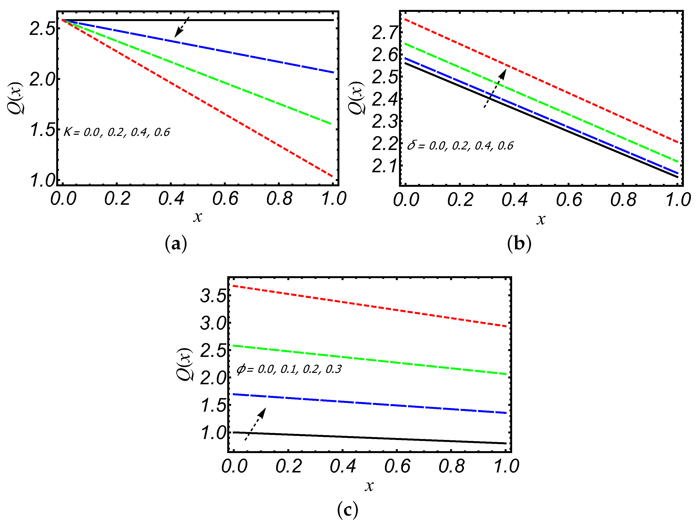
The axial flow rate is obtained using the summarized solution as

$$\begin{array}{ccc}Q\left(x\right)\hfill & =& 2W{\int }_0^H\left(u(x,y)\right)dy,\hfill \\ & =& \frac{b_1(Q_0-2W{V}_{0}x)}{70}\left(-35+105b_2+6{b_1}^2(-1+3b_1{b}_3-2b_1{b}_4){\delta }^2\right).\hfill \end{array}$$

(79)

Here, the dependence of $Q\left(x\right)$ on $\delta$ is only due to the presence of $\varphi$, if $\varphi =0$ then

$$\begin{array}{c}Q\left(x\right)=\left(Q_0-2W{V}_{0}x\right)\hfill \end{array}$$

(d)

The leakage flux $q\left(x\right)$ is obtained as

$$\begin{array}{ccc}q\left(x\right)\hfill & =& -{\displaystyle \frac{dQ}{dx}},\hfill \\ & =& \frac{b_{1}W{V}_0}{35}(-35+105b_2+6{b_1}^2(-1+3b_1{b}_3-2b_1{b}_4){\delta }^2)).\hfill \end{array}$$

(80)

(e)

The fractional reabsorption $F_a$ is obtained as

$$\begin{array}{ccc}{F}_a\hfill & =& {\displaystyle \frac{1}{Q\left(0\right)}}\left(Q\left(0\right)-Q\left(L\right)\right),\hfill \\ & =& \frac{2LW{V}_0}{Q_0}.\hfill \end{array}$$

(81)

The contribution of $\delta$ in leakage flux $q\left(x\right)$ is only due to $\varphi$ and $F_a$ is only influenced by absorption parameter.

(f)

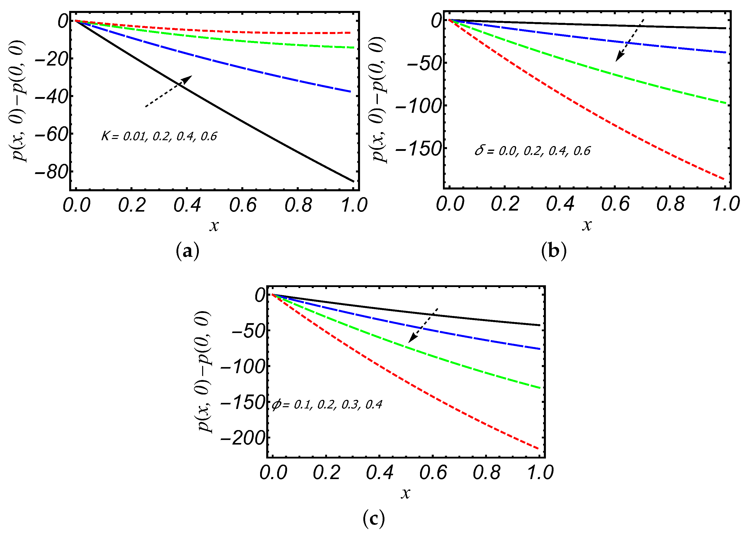
Pressure Distribution

Here, we will find out the pressure for each order by utilizing Equations (30) and (31) into Equations (15)–(17) to get the pressure for the first order

$$\begin{array}{ccc}{\displaystyle \frac{\partial p^{\left(1\right)}}{\partial x}}\hfill & =& -\frac{3b_1\mu \left(Q_0-2Wx{V}_0\right)}{2H^{3}W},\hfill \end{array}$$

(82)

$$\begin{array}{ccc}{\displaystyle \frac{\partial p^{\left(1\right)}}{\partial y}}\hfill & =& -\frac{3b_1\mu y{V}_0}{H^3}.\hfill \end{array}$$

(83)

Equation (82) on integration with respect to x yields

$$p^{\left(1\right)}=-\frac{3b_1\mu \left(x{Q}_0-W{x}^2{V}_0\right)}{2H^{3}W}+B\left(y\right),$$

(84)

where the unknown function $B\left(y\right)$ is to be determined as follows:

Differentiating Equation (84) with respect to y, and on comparing with Equation (83), gives

$$B^{\prime }\left(y\right)=-\frac{3b_1\mu y{V}_0}{H^3},$$

(85)

Then, Equation (84) becomes

$$p^{\left(1\right)}-p_0^{\left(1\right)}=-\frac{3b_1\mu \left(x{Q}_0-W{x}^2{V}_0\right)}{2H^{3}W}-\frac{3b_1\mu y^2{V}_0}{2H^3},$$

(86)

where $p_0^{\left(1\right)}=p(0,0)$ is the pressure at $(x,y)=(0,0)$, i.e., the entrance region of the slit.

The mean pressure is obtained as

$$\begin{array}{ccc}{\overline{p}}^{\left(1\right)}\left(x\right)\hfill & =& \frac{1}{H}{\int }_0^H(p^{\left(1\right)}-p_0^{\left(1\right)})dy,\hfill \\ & =& \frac{b_1\mu }{2H}\left(\frac{3x\left(Wx{V}_0-Q_0\right)}{H^{2}W}-V_0\right),\hfill \end{array}$$

(87)

The pressure drop over slit length L is obtained as

$$\begin{array}{ccc}\Delta {\overline{p}}^1\left(L\right)\hfill & =& \left({\overline{p}}^1\left(0\right)-{\overline{p}}^1\left(L\right)\right),\hfill \\ & =& \frac{3{\mathrm{b}}_1\mu L\left(Q_0-LW{V}_0\right)}{2H^{3}W}.\hfill \end{array}$$

(88)

Similarly, we can obtain

$$\begin{array}{ccc}{p}^{\left(2\right)}-p_0^{\left(2\right)}\hfill & =& \frac{3b_1^2\delta \mu }{2H}\left(\frac{3b_{2}x\left(-Q_0+Wx{v}_0\right)}{H^{2}W}-3b_2{v}_0{\left(\frac{y}{H}\right)}^2+2v_0{\left(\frac{y}{H}\right)}^4\right),\hfill \end{array}$$

(89)

$$\begin{array}{ccc}{\overline{p}}^{\left(2\right)}\left(x\right)\hfill & =& \frac{3b_1^2\delta \mu }{10H}\left(\frac{15b_{2}x\left(-Q_0+Wx{v}_0\right)}{H^{2}W}+(2-5b_2)v_0\right),\hfill \end{array}$$

(90)

$$\begin{array}{ccc}\Delta {\overline{p}}^2\left(L\right)\hfill & =& \frac{9{\mathrm{b}1}^2\mathrm{b}2L\delta \mu \left(Q_0-LW{v}_0\right)}{2H^{3}W}\hfill \end{array}$$

(91)

$$\begin{array}{ccc}{p}^{\left(3\right)}-p_0^{\left(3\right)}\hfill & =& \frac{9b_1^3{\delta }^2\mu }{70H}(-28V_0{(\frac{y}{H})}^6+(3\left(-35b_2^2+2b_1{b}_3\right)V_0){\left(\frac{y}{H}\right)}^2\hfill \\ & -& \frac{3x\left(Q_0-Wx{V}_0\right)}{H^{2}W}(\left(35b_2^2-2b_1{b}_3\right))),\hfill \end{array}$$

(92)

$$\begin{array}{ccc}{\overline{p}}^{\left(3\right)}\left(x\right)\hfill & =& \frac{9b_1^3{\delta }^2\mu }{70H}(\frac{3x\left(Q_0-Wx{V}_0\right)}{H^{2}W}(-35b_2^2+2b_1{b}_3)+(-4\hfill \\ & & -35b_2^2+2b_1{b}_3)V_0)\hfill \end{array}$$

(93)

$$\begin{array}{ccc}\Delta {\overline{p}}^3\left(L\right)\hfill & =& \frac{27b_1^{3}L{\delta }^2\mu \left(Q_0-LW{v}_0\right)}{70H^{3}W}\left(35b_2^2-2b_1{b}_3\right)\hfill \end{array}$$

(94)

Here, we note that the pressure field has considerable contribution from viscoelastic effect for the second order even though the velocity field had zero contribution at that order.

The summarized forms of total pressure difference, mean pressure and pressure drop are given as

$$\begin{array}{ccc}p(x,y)-p(0,0)\hfill & =& \frac{3b_1\mu v_0}{70H}(-84{b_1}^2{\delta }^2{\left(\frac{y}{H}\right)}^6+70b_1\delta {\left(\frac{y}{H}\right)}^4+(-35-105b_1{b}_2\delta \hfill \\ & +& \left(-315{b_1}^2{b_2}^2+18{b_1}^3{b}_3\right){\delta }^2)){\left(\frac{y}{H}\right)}^2)+\frac{3b_{1}x\mu \left(Q_0-Wx{v}_0\right)}{70H^{3}W}(\hfill \\ & -& 35-105b_1{b}_2\delta +\left(-315{b_1}^2{b_2}^2+18{b_1}^3{b}_3\right){\delta }^2)\hfill \end{array}$$

(95)

$$\begin{array}{ccc}\overline{p}\left(x\right)\hfill & =& b_1\mu (\frac{3x\left(Q_0-Wx{v}_0\right)}{70H^{3}W}(-35-105b_1{b}_2\delta +(-315{b_1}^2{b_2}^2\hfill \\ & +& 18{b_1}^3{b}_3){\delta }^2)+\frac{v_0}{70H}(-35+(42b_1-105b_1{b}_2)\delta +9{b_1}^2(-4-35{b_2}^2\hfill \\ & +& 2b_1{b}_3){\delta }^2))\hfill \end{array}$$

(96)

$$\begin{array}{ccc}\Delta \overline{p}\left(L\right)\hfill & =& \frac{3b_{1}L\mu \left(-Q_0+LW{v}_0\right)}{70H^{3}W}(-35-105\mathrm{b}1\mathrm{b}2\delta +(-315{\mathrm{b}1}^2{\mathrm{b}2}^2\hfill \\ & +& 18{\mathrm{b}1}^3\mathrm{b}3){\delta }^2)\hfill \end{array}$$

(97)

We noticed that $p(x,y)$, $\Delta \overline{p}\left(L\right)$ and $\overline{p}\left(x\right)$ are varying with slip coefficient $\varphi$, and Maxwell parameter $\delta$. In the limiting case, when $\varphi =0,\delta =0$, we recovered the exact expressions of $p(x,y)$, $\Delta \overline{p}\left(L\right)$ and $\overline{p}\left(x\right)$ of a Newtonian fluid [15].

(g)

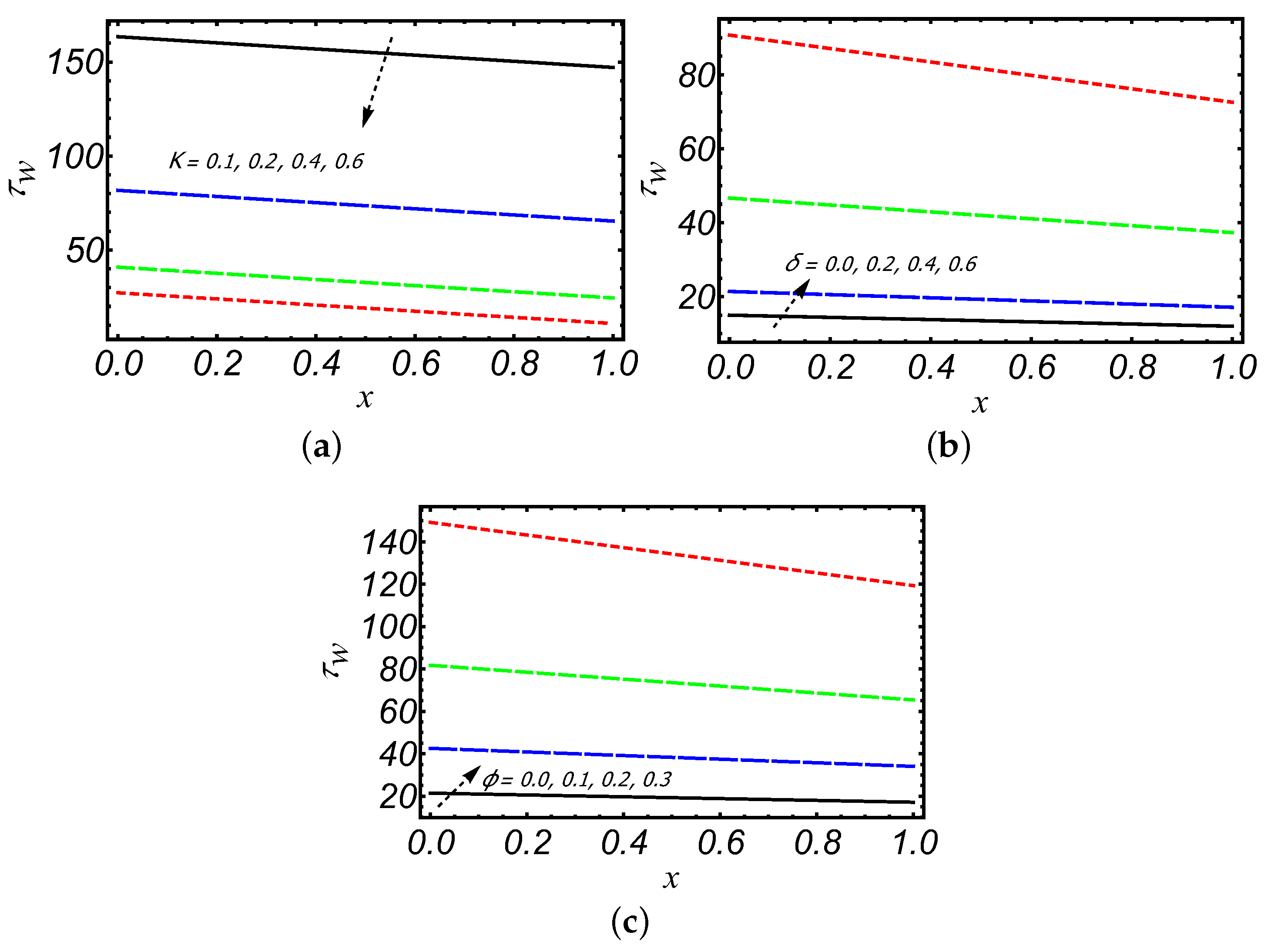
The wall shear stress is obtained as

$$\begin{array}{ccc}{\tau }_w=-{\tau }_{xy}{|}_{y=H}\hfill & =& \frac{3b_1\mu \left(Q_0-2Wx{V}_0\right)}{70H^{2}W}(35+35b_1(-4+3b_2)\delta +9{b_1}^2(28+35{b_2}^2\hfill \\ & -& 2b_1{b}_3){\delta }^2).\hfill \end{array}$$

(98)

(h)

The expressions for normal stress differences are given as

$$\begin{array}{ccc}{\tau }_n={\tau }_{xx}-{\tau }_{yy}\hfill & =& \frac{3b_1\mu v_0}{70H}(1596{b_1}^2{\delta }^2{(\frac{y}{H})}^6-35b_1(-4\delta +144b_1{b}_2{\delta }^2\hfill \\ & & +\frac{9b_1{\delta }^2\left(Q_0-2Wx{v}_0\right){}^2}{H^2{W}^2{v}_0{}^2}){(\frac{y}{H})}^4+(140-420b_1{b}_2\delta -72{b_1}^2(-70{b_2}^2\hfill \\ & & +b_1{b}_3){\delta }^2+\frac{105b_1\delta \left(Q_0-2Wx{v}_0\right){}^2}{H^2{W}^2{v}_0{}^2})\hfill \\ & & {(\frac{y}{H})}^2-140b_2-4{b_1}^2(315{b_2}^3-4b_1{b}_4){\delta }^2)\hfill \end{array}$$

(99)

$$\begin{array}{ccc}{\tau }_n{|}_{y=H}\hfill & =& \frac{3b_1\mu v_0}{70H}(-140(-1+b_2)+140b_1(1-3b_2)\delta +4{b_1}^2(399\hfill \\ & -& 315{(-2+b_2)}^2{b}_2-18b_1{b}_3+4b_1{b}_4){\delta }^2\hfill \\ & & -\frac{105b_1\delta (-1+3b_1\delta )\left(Q_0-2Wx{v}_0\right){}^2}{H^2{W}^2{v}_0^2}),\hfill \end{array}$$

(100)

$$\begin{array}{ccc}{\tau }_n{|}_{y=0}\hfill & =& \frac{3b_1\mu v_0}{70H}(-140b_2+4{b_1}^2\left(-315{b_2}^3+4b_1{b}_4\right){\delta }^2).\hfill \end{array}$$

(101)

4. Discussion

In the present article, we have successfully implemented the recursive approach to linearize the full momentum equations describing the incompressible slow flow of a Maxwell fluid between two porous walls and analytical solutions for stream function, velocity components, total pressure difference, explicit expressions for normal and shear stresses, volumetric flow rate, fractional absorption and leakage flux are calculated. To predict the impact of pertinent parameters like absorption parameter K, slip parameter $\varphi$ and Maxwell fluid parameter $\delta$ on flow variables, we first used the following dimensionless parameters and then we established different graphs after removing star along the three different places along slit length, i.e., entrance region (x = 0.1), middle region (x = 0.5) and exit region (x = 0.9).

$$\begin{array}{ccc}\hfill & \hfill & x^{*}={\displaystyle \frac{x}{H}},\zeta ={\displaystyle \frac{y}{H}},u^{*}={\displaystyle \frac{u}{Q_0/WH}},v^{*}={\displaystyle \frac{v}{Q_0/WH}},\hfill \\ \hfill & \hfill & p^{*}={\displaystyle \frac{p}{\mu V_0/H}},{{\tau }^{*}}_{ij}={\displaystyle \frac{{\tau }_{ij}}{\mu V_0/H}}K=\frac{2HW{V}_0}{Q_0},Q^{*}\left(x\right)=\frac{Q\left(x\right)}{Q_0}.\hfill \end{array}$$

(102)

Figure 2, Figure 3 and Figure 4 are drawn to see the impact of porosity K on $u\left(\zeta \right)$ for the creeping flow of Newtonian and non-Newtonian (Maxwell) fluids. It is justified that when we increase the value of porosity K, the wall permeability increases and more fluid passed through the slit walls which causes an increase in magnitude of the seepage velocity. Keeping this fact in mind, we see that these figures depicted a decrease in axial velocity $u\left(\zeta \right)$ on increasing porosity K and the magnitude of axial velocity also reduces downstream throughout the channel. For large values of K, a reversal flow may occur near the exit region of the slit. A standard parabolic velocity profile for Poiseuille flow in the absence of porosity throughout the channel is also observed in Figure 2. An increase is also observed in magnitude of axial velocity profile due to the presence of $\varphi$ in Figure 4. A clear difference can be observed in velocity profiles for slow flow of Newtonian and Maxwell fluids in Figure 3 and Figure 4.

Figure 5 and Figure 6 show the impact of Maxwell fluid parameter $\delta$ on the axial velocity $u\left(\zeta \right)$ of creeping Maxwell fluid with and without slip parameter, keeping $K=0.2$. It is viewed that on increasing value of $\delta$, the shear thickening property is observed along the centerline of the slit as axial velocity $u\left(\zeta \right)$ decreases along the centerline of the slit and due to reabsorption and slip effects on the slit wall, the shear thinning property of the fluid near the wall is observed as $u\left(\zeta \right)$ increases near the slit wall. An increase in the magnitude of $u\left(\zeta \right)$ can be seen due to parameter $\varphi$ in Figure 6.

Figure 7 and Figure 8 reveal the impact of parameter $\varphi$ on $u\left(\zeta \right)$ in Newtonian and non-Newtonian cases. It is viewed that the velocity of fluid at the boundary is not the same velocity with fluid particles closet to the wall. In both cases with increasing the slip parameter $\varphi$, $u\left(\zeta \right)$ increases. The variation in the radial velocity component $v\left(\zeta \right)$ can be seen in Figure 9 and we have observed that $v\left(\zeta \right)$ increases as we increased the parameters K and $\varphi$, whereas it is decreasing due to $\delta$.

Figure 10, Figure 11 and Figure 12 are drawn to show the impact of pertinent parameters on pressure $p(x,y)$, shear stress ${\tau }_w$ and normal stress difference ${\tau }_n$ of a creeping Maxwell fluid. It is noted that in Figure 10, the pressure difference is increasing due to K and decreasing downstream on increasing $\delta$ and $\varphi$, whereas Figure 11 illustrate that the wall shear stress ${\tau }_w$ has opposite effects as compared to pressure difference due to these parameters.

It is also noted in Figure 12a that porosity K does not affect the normal stress difference ${\tau }_n$ away from boundaries but ${\tau }_n$ decreases near the walls with K and also in Figure 12b,c ${\tau }_n$ decreases on increasing $\delta$ and $\varphi$. Figure 13 shows the variation of $Q\left(x\right)$ and it is depicted that $Q\left(x\right)$ decreases as we increased porosity K whereas it is increasing as we increase parameters $\delta$ and $\varphi$.

5. Conclusions

In this article, we have presented the slow flow of a Maxwell fluid through the permeable slit under the influence of a slip condition and the recursive approach is consider to get an analytical solution. The key features of the current investigation were the impact of parameters K, $\varphi$ and $\delta$ on flow variables involved. Moreover, the recursive approach is used for the first time to deal with a rate type Maxwell fluid creeping flow and the obtained results are very similar to existing results presented by [15] in a limiting case with certain restricted conditions. The following outcomes are drawn from this study:

• If the Maxwell fluid parameter $\delta =0$ and slip parameter $\varphi =0$, then results obtained by Haroon [15] are recovered.
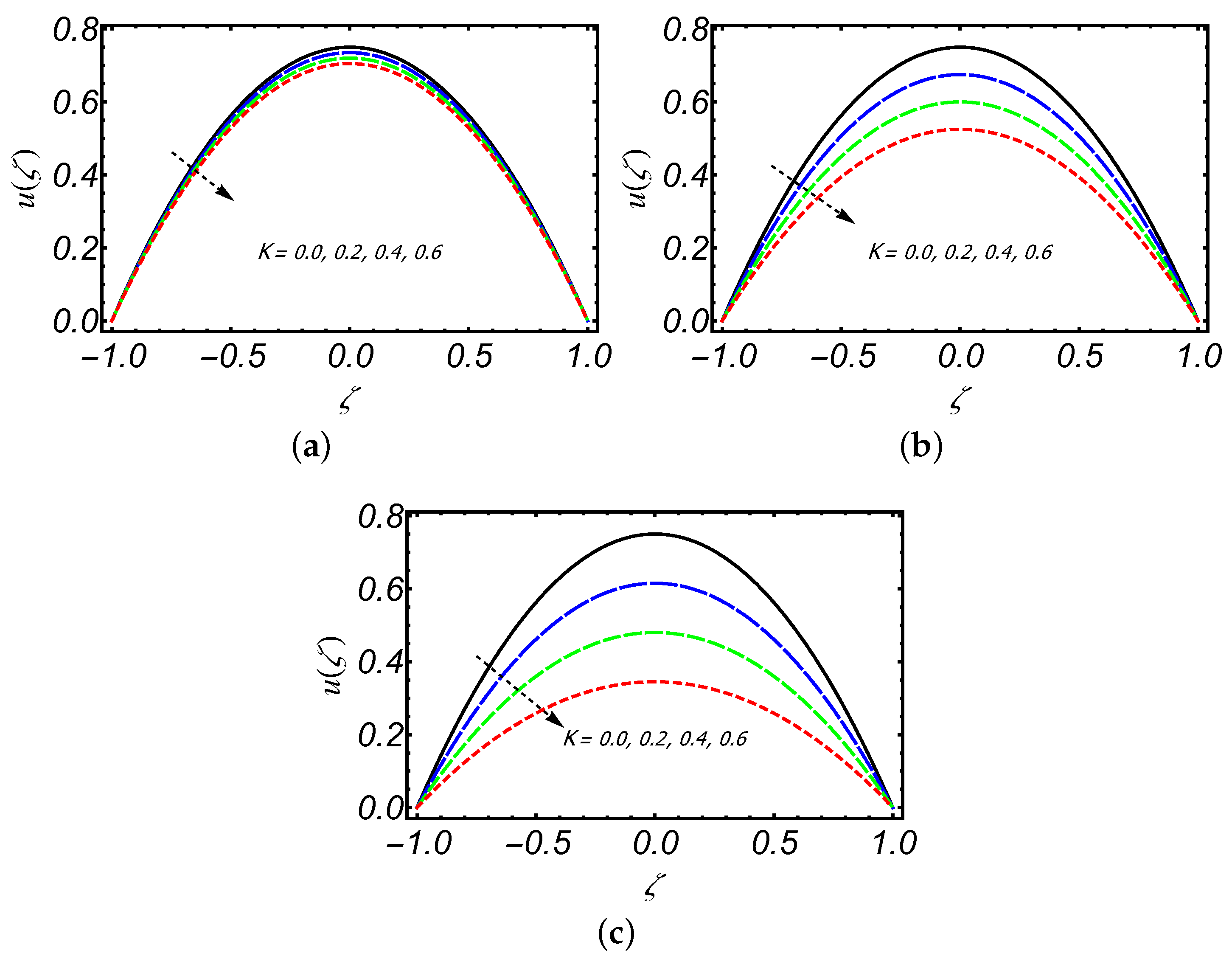
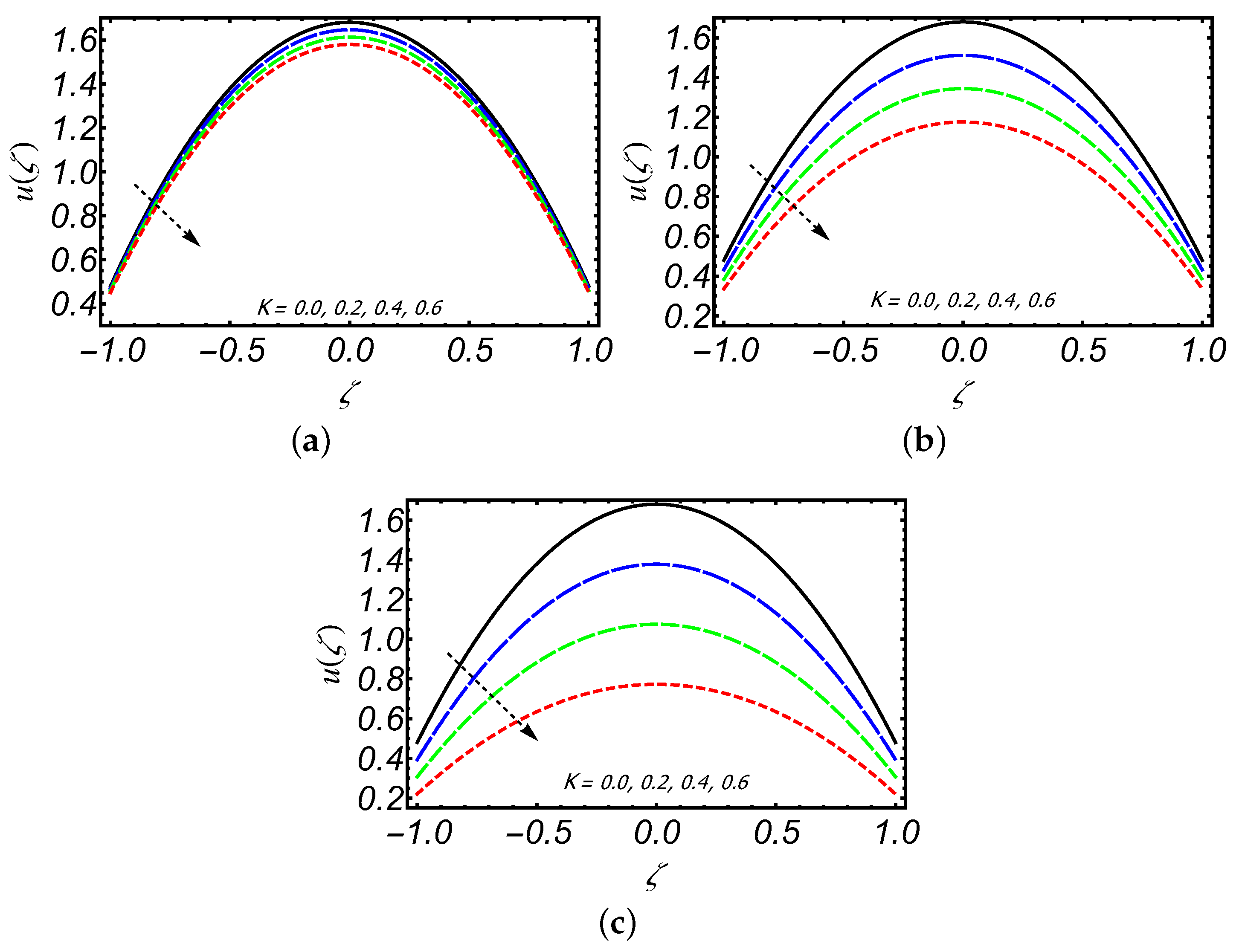
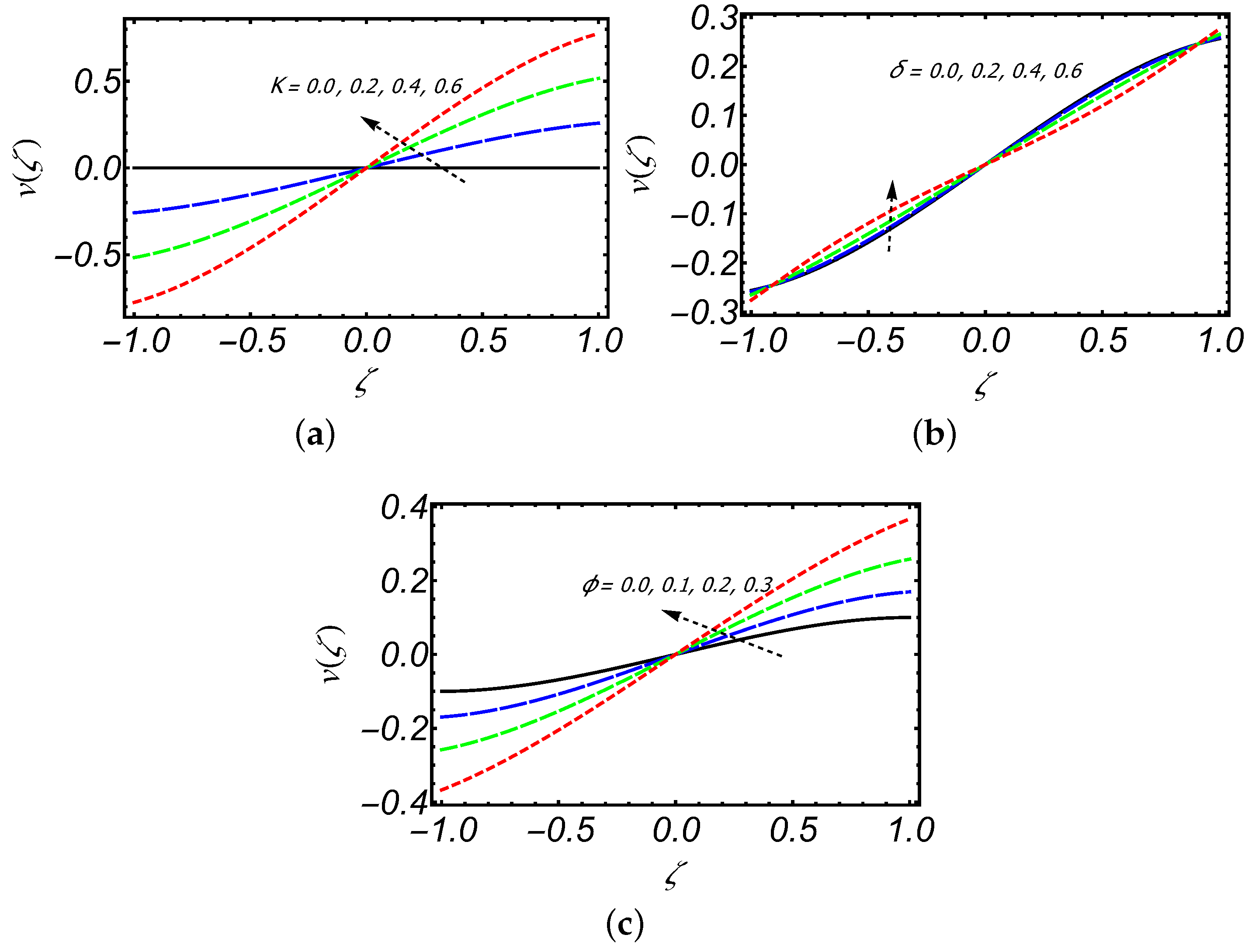
• The axial velocity $u\left(\zeta \right)$ of creeping Maxwell fluid decreases downstream along the slit length on increasing porosity K and also for increasing values of K, backward flow can be seen near the exit region of the slit.
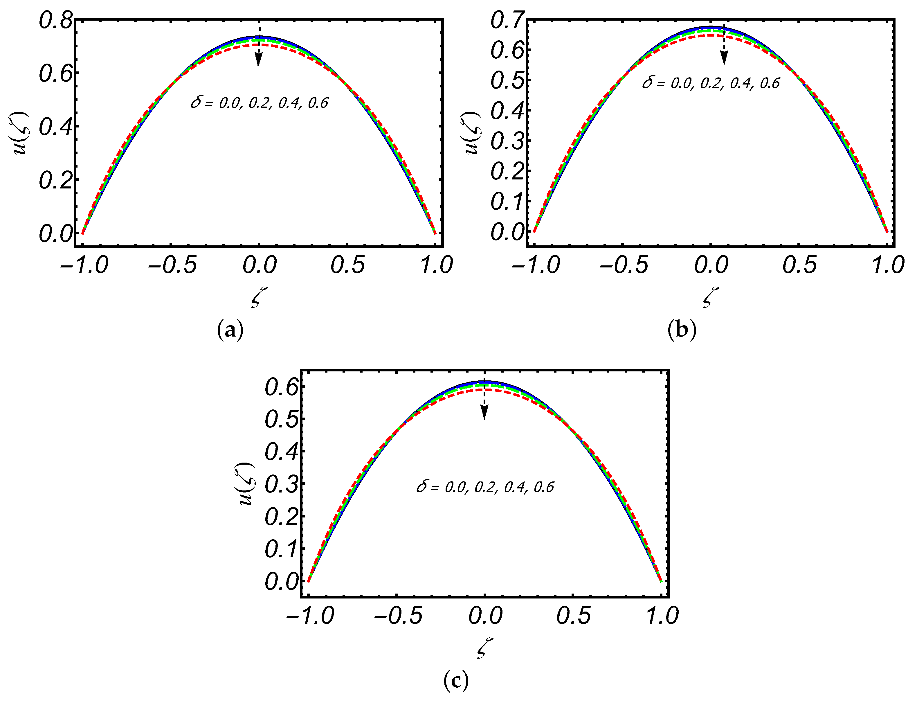
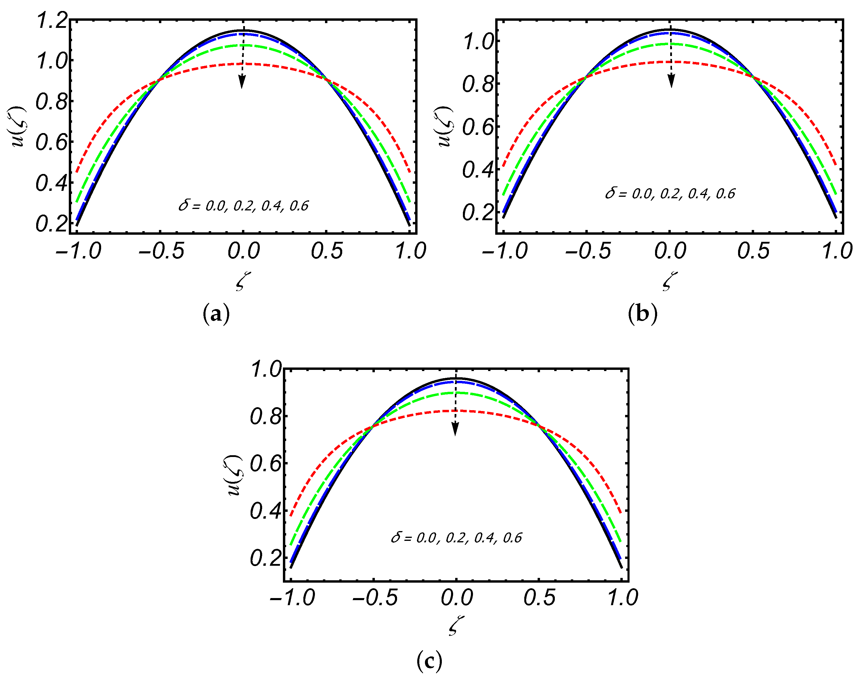
• The axial velocity profile has an increasing behavior near the slit walls and its decreasing trend is observed along the centerline of the slit with increasing $\delta$.
• The shear thickening and thinning behavior of the Maxwell fluid is observed along centerline and near the walls of the slit, respectively.
• Along the slit length, the magnitude of $u\left(\zeta \right)$ decreases as the fluid moves from the entrance to exit region of the slit.
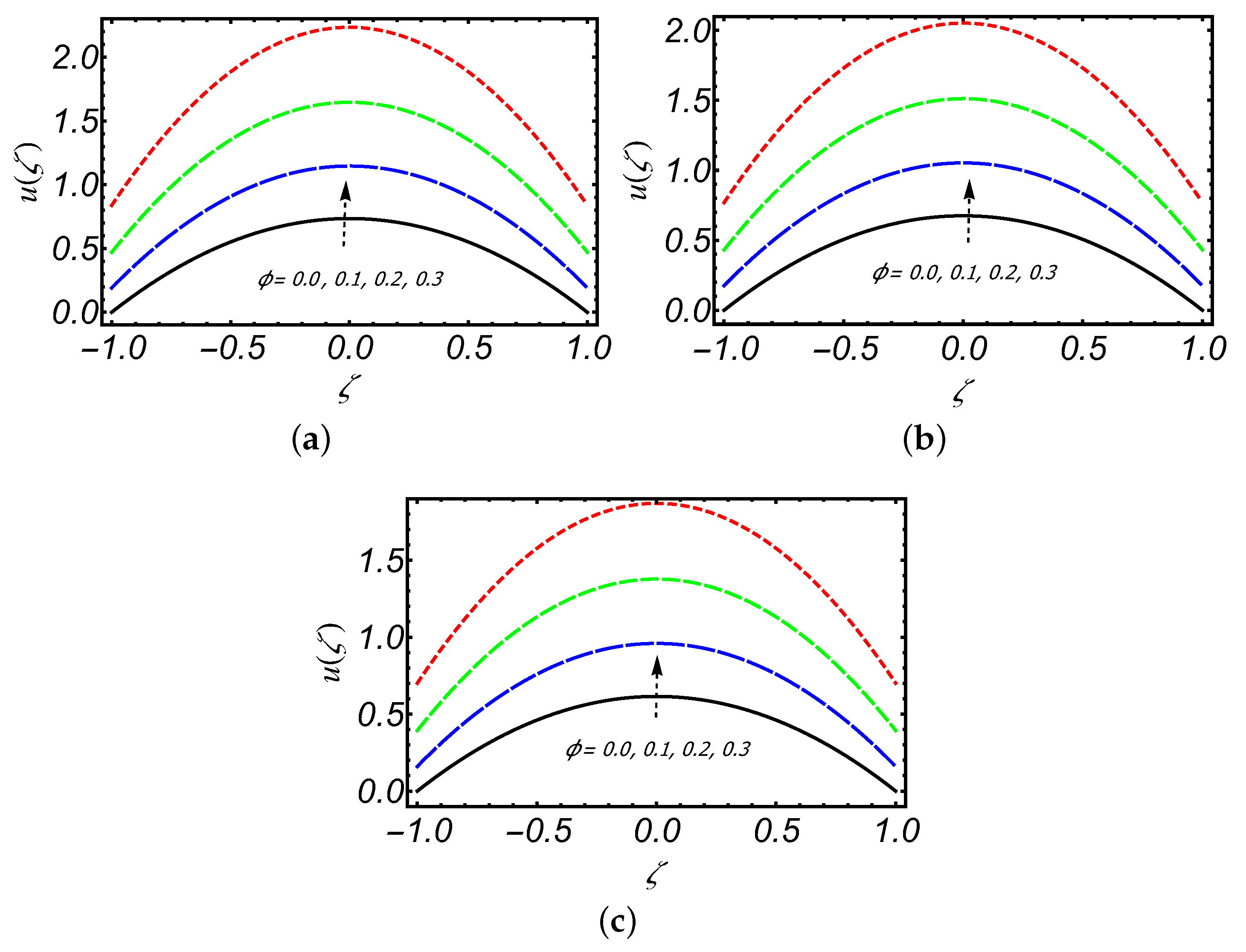
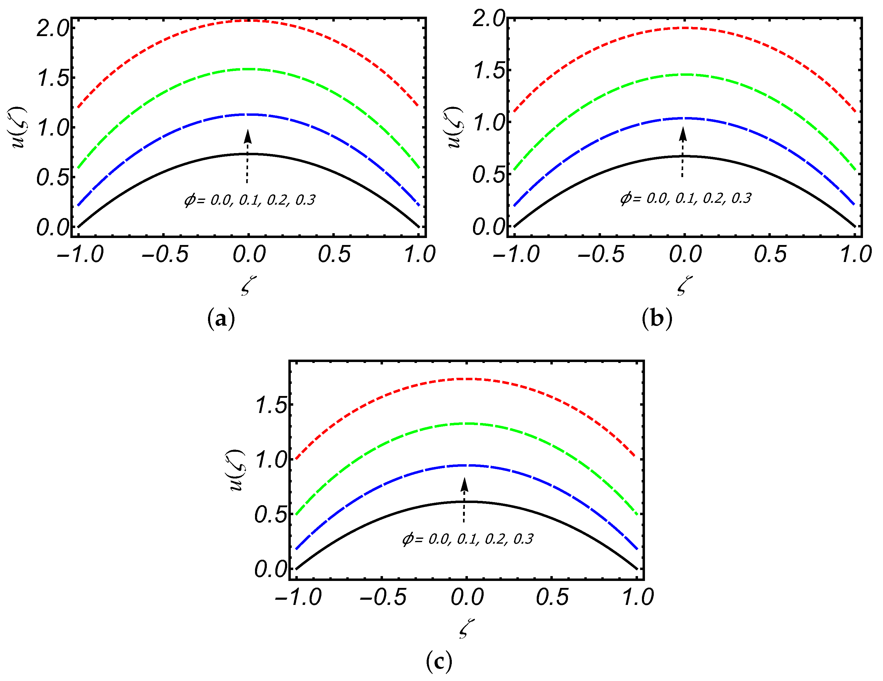
• An increase in axial velocity of a creeping Maxwell fluid is observed due to the increasing value of $\varphi$.
• The slip parameter $\varphi$ significantly influenced the magnitude of axial and radial velocities in comparison to other parameters.
• A decreasing trend in pressure profile for increasing values of $\varphi$ and $\delta$, whereas pressure is increasing with increasing porosity parameter K.
• The wall shear stress ${\tau }_w$ is increasing significantly by increasing $\delta$ and $\varphi$, but with K and ${\tau }_w$ decreasing.
• The contribution of $\delta$ in axial flow rate and leakage flux is only due to the presence of a slip parameter $\varphi$.

References

- Nikolay, V. Desalination Engineering: Planning and Design; McGraw-Hill Professional: New York, NY, USA, 2013. [Google Scholar]
- Espedal, M.S.; Mikelic, A. Filtration in Porous Media and Industrial Application: Lectures Given at the 4th Session of the Centro Internazionale Matematico Estivo (CIME) Held in Cetraro, Italy, 24–29 August 1998; Springer: New York, NY, USA, 2007. [Google Scholar]
- Macey, R.I. Pressure flow patterns in a cylinder with reabsorbing walls. Bull. Math. Biophys. 1963, 25, 1–9. [Google Scholar] [CrossRef]
- Macey, R.I. Hydrodynamics in the renal tubule. Bull. Math. Biophys. 1965, 27, 117. [Google Scholar] [CrossRef] [PubMed]
- Marshall, E.; Trowbridge, E. Flow of a Newtonian fluid through a permeable tube: The application to the proximal renal tubule. Bull. Math. Biol. 1974, 36, 457–476. [Google Scholar] [CrossRef]
- Marshall, E.; Trowbridge, E.; Aplin, A. Flow of a Newtonian fluid between parallel flat permeable plates, The application to a flat plate hemodialyzer. Math. Biosci. 1975, 27, 119–139. [Google Scholar] [CrossRef]
- Berman, A.S. Laminar flow in channels with porous walls. J. Appl. Phys. 1953, 24, 1232–1235. [Google Scholar] [CrossRef]
- Sellars, J.R. Laminar flow in channels with porous walls at high suction Reynolds numbers. J. Appl. Phys. 1955, 26, 489–490. [Google Scholar] [CrossRef]
- Yuan, S. Further investigation of laminar flow in channels with porous walls. J. Appl. Phys. 1956, 27, 267–269. [Google Scholar] [CrossRef]
- Wah, T. Laminar flow in a uniformly porous channel. Aeronaut. Q. 1964, 15, 299–310. [Google Scholar] [CrossRef]
- Terrill, R. Laminar flow in a uniformly porous channel with large injection. Aeronaut. Q. 1965, 16, 323–332. [Google Scholar] [CrossRef]
- Karode, S.K. Laminar flow in channels with porous walls revisited. J. Membr. Sci. 2001, 191, 237–241. [Google Scholar] [CrossRef]
- Siddiqui, A.M.; Haroon, T.; Shahzad, A. Hydrodynamics of viscous fluid through porous slit with linear absorption. Appl. Math. Mech. 2016, 37, 361–378. [Google Scholar] [CrossRef]
- Haroon, T.; Siddiqui, A.M.; Shahzad, A. Stokes flow through a slit with periodic reabsorption: An application to renal tubule. Alex. Eng. J. 2016, 55, 1799–1810. [Google Scholar] [CrossRef]
- Haroon, T.; Siddiqui, A.; Shahzad, A. Creeping flow of viscous fluid through a proximal tubule with uniform reabsorption: A mathematical study. Appl. Math. Sci. 2016, 10, 795–807. [Google Scholar] [CrossRef]
- Haroon, T.; Siddiqui, A.; Shahzad, A.; Smeltzer, J. Steady creeping slip flow of viscous fluid through a permeable slit with exponential reabsorption1. Appl. Math. Sci. 2017, 11, 2477–2504. [Google Scholar]
- Rajagopal, K. On the creeping flow of the second-order fluid. J. Non-Newton. Fluid Mech. 1984, 15, 239–246. [Google Scholar] [CrossRef]
- Ullah, H.; Sun, H.; Siddiqui, A.M.; Haroon, T. Creeping flow analysis of slightly non-Newtonian fluid in a uniformly porous slit. J. Appl. Anal. Comput. 2019, 9, 140–158. [Google Scholar] [CrossRef]
- Ullah, H.; Siddiqui, A.M.; Sun, H.; Haroon, T. Slip effects on creeping flow of slightly non-Newtonian fluid in a uniformly porous slit. J. Braz. Soc. Mech. Sci. Eng. 2019, 41, 412. [Google Scholar] [CrossRef]
- Kahshan, M.; Siddiqui, A.; Haroon, T. A micropolar fluid model for hydrodynamics in the renal tubule. Eur. Phys. J. Plus 2018, 133, 546. [Google Scholar] [CrossRef]
- Kahshan, M.; Lu, D.; Siddiqui, A. A Jeffrey fluid model for a porous-walled channel: Application to flat plate dialyzer. Sci. Rep. 2019, 9, 1–18. [Google Scholar] [CrossRef]
- Lu, D.; Kahshan, M.; Siddiqui, A. Hydrodynamical study of micropolar fluid in a porous-walled channel: Application to flat plate dialyzer. Symmetry 2019, 11, 541. [Google Scholar] [CrossRef]
- Langlois, W. A Recursive Approach to the Theory of Slow, Steady-State Viscoelastic Flow. Trans. Soc. Rheol. 1963, 7, 75–99. [Google Scholar] [CrossRef]
- Langlois, W. The recursive theory of slow viscoelastic flow applied to three basic problems of hydrodynamics. Trans. Soc. Rheol. 1964, 8, 33–60. [Google Scholar] [CrossRef]
- Léger, L.; Hervet, H.; Massey, G.; Durliat, E. Wall slip in polymer melts. J. Phys. Condens. Matter 1997, 9, 7719. [Google Scholar] [CrossRef]
- Atwood, B.; Schowalter, W. Measurements of slip at the wall during flow of high-density polyethylene through a rectangular conduit. Rheol. Acta 1989, 28, 134–146. [Google Scholar] [CrossRef]
- Beavers, G.S.; Joseph, D.D. Boundary conditions at a naturally permeable wall. J. Fluid Mech. 1967, 30, 197–207. [Google Scholar] [CrossRef]
- Saffman, P.G. On the boundary condition at the surface of a porous medium. Stud. Appl. Math. 1971, 50, 93–101. [Google Scholar] [CrossRef]
- Beavers, G.S.; Sparrow, E.M.; Magnuson, R.A. Experiments on coupled parallel flows in a channel and a bounding porous medium. J. Basic Eng. 1970, 92, 843–848. [Google Scholar] [CrossRef]
- Kohler, J.T. An Investigation of Laminar Flow through a Porous Walled Channel: I. A Perturbation Solution Assuming Slip at the Permeable Wall. II. An Experimental Measurement of the Velocity Distribution Utilizing a Dye Tracer Technique. Ph.D. Thesis, University of Massachusetts Amherst, Amherst, MA, USA, 1974. [Google Scholar]
- Mikelic, A.; Jäger, W. On the interface boundary condition of Beavers, Joseph, and Saffman. SIAM J. Appl. Math. 2000, 60, 1111–1127. [Google Scholar] [CrossRef]
- Rao, I.; Rajagopal, K. The effect of the slip boundary condition on the flow of fluids in a channel. Acta Mech. 1999, 135, 113–126. [Google Scholar] [CrossRef]
- Elshahed, M. Blood flow in capillary under starling hypothesis. Appl. Math. Comput. 2004, 149, 431–439. [Google Scholar] [CrossRef]
- Singh, R.; Laurence, R.L. Influence of slip velocity at a membrane surface on ultrafiltration performance I. Channel flow system. Int. J. Heat Mass Transf. 1979, 22, 721–729. [Google Scholar] [CrossRef]
- Makinde, O.; Osalusi, E. MHD steady flow in a channel with slip at the permeable boundaries. Rom. J. Phys. 2006, 51, 319. [Google Scholar]
- Eldesoky, I.M. Unsteady MHD pulsatile blood flow through porous medium in a stenotic channel with slip at the permeable walls subjected to time dependent velocity (injection/suction). In Proceedings of the International Conference on Mathematics and Engineering Physics, Kobry Elkobbah, Egypt, 29–31 May 2014; Volume 7, pp. 1–25. [Google Scholar]
- El-Shehawy, E.; El-Dabe, N.; El-Desoky, I. Slip effects on the peristaltic flow of a non-Newtonian Maxwellian fluid. Acta Mech. 2006, 186, 141–159. [Google Scholar] [CrossRef]
- Ellahi, R. Effects of the slip boundary condition on non-Newtonian flows in a channel. Commun. Nonlinear Sci. Numer. Simul. 2009, 14, 1377–1384. [Google Scholar] [CrossRef]
- Hron, J.; Le Roux, C.; Málek, J.; Rajagopal, K. Flows of incompressible fluids subject to Naviers slip on the boundary. Comput. Math. Appl. 2008, 56, 2128–2143. [Google Scholar] [CrossRef]
- Hayat, T.; Khan, M.; Ayub, M. The effect of the slip condition on flows of an Oldroyd 6-constant fluid. J. Comput. Appl. Math. 2007, 202, 402–413. [Google Scholar] [CrossRef][Green Version]
- Rajagopal, K.R.; Srinivasa, A.R. A thermodynamic frame work for rate type fluid models. J. Non-Newton. Fluid Mech. 2000, 88, 207–227. [Google Scholar] [CrossRef]
- Choi, J.; Rusak, Z.; Tichy, J. Maxwell fluid suction flow in a channel. J. Non-Newton. Fluid Mech. 1999, 85, 165–187. [Google Scholar] [CrossRef]
- Sadeghy, K.; Najafi, A.H.; Saffaripour, M. Sakiadis flow of an upper-convected Maxwell fluid. Int. J. Non-Linear Mech. 2005, 40, 1220–1228. [Google Scholar] [CrossRef]
- Abbas, Z.; Sajid, M.; Hayat, T. MHD boundary-layer flow of an upper-convected Maxwell fluid in a porous channel. Theor. Comput. Fluid Dyn. 2006, 20, 229–238. [Google Scholar] [CrossRef]
- Bhatti, K.; Siddiqui, A.M.; Bano, Z. Application of Recursive Theory of Slow Viscoelastic Flow to the Hydrodynamics of Second-Order Fluid Flowing through a Uniformly Porous Circular Tube. Mathematics 2020, 8, 1170. [Google Scholar] [CrossRef]
Publisher’s Note: MDPI stays neutral with regard to jurisdictional claims in published maps and institutional affiliations. |
© 2020 by the authors. Licensee MDPI, Basel, Switzerland. This article is an open access article distributed under the terms and conditions of the Creative Commons Attribution (CC BY) license (http://creativecommons.org/licenses/by/4.0/).
Share and Cite
Ullah, H.; Lu, D.; Siddiqui, A.M.; Haroon, T.; Maqbool, K. Hydrodynamical Study of Creeping Maxwell Fluid Flow through a Porous Slit with Uniform Reabsorption and Wall Slip. Mathematics 2020, 8, 1852. https://doi.org/10.3390/math8101852
Ullah H, Lu D, Siddiqui AM, Haroon T, Maqbool K. Hydrodynamical Study of Creeping Maxwell Fluid Flow through a Porous Slit with Uniform Reabsorption and Wall Slip. Mathematics. 2020; 8(10):1852. https://doi.org/10.3390/math8101852
Chicago/Turabian StyleUllah, Hameed, Dianchen Lu, Abdul Majeed Siddiqui, Tahira Haroon, and Khadija Maqbool. 2020. "Hydrodynamical Study of Creeping Maxwell Fluid Flow through a Porous Slit with Uniform Reabsorption and Wall Slip" Mathematics 8, no. 10: 1852. https://doi.org/10.3390/math8101852
APA StyleUllah, H., Lu, D., Siddiqui, A. M., Haroon, T., & Maqbool, K. (2020). Hydrodynamical Study of Creeping Maxwell Fluid Flow through a Porous Slit with Uniform Reabsorption and Wall Slip. Mathematics, 8(10), 1852. https://doi.org/10.3390/math8101852