Article

Linear Convergence of Split Equality Common Null Point Problem with Application to Optimization Problem

School of Mathematical Sciences, Tiangong University, Tianjin 300392, China
*
Author to whom correspondence should be addressed.
Mathematics 2020, 8(10), 1836; https://doi.org/10.3390/math8101836
Submission received: 25 August 2020 / Revised: 14 October 2020 / Accepted: 15 October 2020 / Published: 19 October 2020
(This article belongs to the Special Issue Nonlinear Problems and Applications of Fixed Point Theory)

Abstract

:
The purpose of this paper is to propose an iterative algorithm for solving the split equality common null point problem (SECNP), which is to find an element of the set of common zero points for a finite family of maximal monotone operators in Hilbert spaces. We introduce the concept of bounded linear regularity for the SECNP and construct several sufficient conditions to ensure the linear convergence of the algorithm. Moreover, some numerical experiments are given to test the validity of our results.

1. Introduction

Let H 1 , H 2 , H 3 be real Hilbert spaces, C and Q be nonempty closed convex subsets of H 1 and H 2 , respectively. Moudafi [1] introduced the following split equality problem (SEP), which is formulated as finding
x C   and   y Q   such   that   A x = B y , ( 1 )
where A : H 1 H 3 and B : H 2 H 3 are two bounded linear operators. When B = I , the SEP reduces to the split feasibility problem (SFP) which was introduced by Censor and Elfving [2]. The SEP allows asymmetric and partial relations between the variables x and y. It has also received much attention due to the application in many disciplines such as medical image reconstruction, game theory, decomposition methods for PDEs and radiation therapy treatment planning; see [3,4,5,6].
In [7], Moudafi introduced and studied the following split equality null point problem (SENP): given two set-valued maximal monotone operators F : H 1 2 H 1 and K : H 2 2 H 2 , the SENP is formulated as finding
x * F 1 ( 0 ) , y * K 1 ( 0 )   such   that   A x * = B y * ,
where F 1 ( 0 ) = { x H 1 : 0 F x } = F i x ( J r F ) is closed and convex, F is set-valued maximal monotone operators [8]. We note that if B = I , this problem reduces to the well-known split common null point problem which was originally introduced by Byrne et al. [9]. For i = 1 , 2 , · · · , m , let { F i } i = 1 m : H 1 2 H 1 and { K i } i = 1 m : H 2 2 H 2 be two families of set-valued maximal monotone operators. The SECNP is formulated as finding
x * F 1 ( 0 ) = i = 1 m F i 1 ( 0 ) , y * K 1 ( 0 ) = i = 1 m K i 1 ( 0 )   such   that   A x * = B y * .
In [7], Moudafi proposed the following algorithm for solving SENP and obtained a weak convergence theorem:
x n + 1 = J r F x n γ n A * ( A x n B y n ) , y n + 1 = J r K y n + γ n B * ( A x n B y n ) , n 0 ,
We note that in the above algorithm, the step-size γ n depends on the operator (matrix) norms A and B (or the largest eigenvalues of A * A and B * B , where A * and B * are the adjoint operators of A and B, respectively). To implement the alternating algorithm (4) for solving SENP (2), we need to compute A and B , which is generally not an easy task in practice.
To overcome this difficulty, Eslamian [10] considered an algorithm for solving SECNP for a finite family of maximal monotone operators which does not require any knowledge of the operator norms. In addition, they presented a strong convergence theorem which is more desirable than weak convergence. The algorithm is as follows:
x n + 1 = β n , 0 ϑ + i = 1 m β n , i J r n , i F i x n γ n A * ( A x n B y n ) , x 0 , ϑ H 1 , y n + 1 = β n , 0 υ + i = 1 m β n , i J s n , i K i y n + γ n B * ( A x n B y n ) , y 0 , υ H 2 , n 0 ,
where i = 0 m β n , i = 1 and γ n = ϵ , 2 A x n B y n 2 B * ( A x n B y n ) 2 + A * ( A x n B y n ) 2 ϵ , n Π , the index set Π = { n : A x n B y n 0 } . In addition, the sequences { β n , i } , { r n , i } and { s n , i } satisfy the following conditions: (i) lim inf n r n , i > 0 , lim inf n s n , i > 0 and lim inf n β n , i > 0 , i { 1 , 2 · · · , m } , (ii) lim n β n , 0 = 0 and n = 0 β n , 0 = . It is proved that the sequence { ( x n , y n ) } generated by algorithm (5) converges strongly to a solution ( x * , y * ) of SECNP (3).
Without loss of generality, let H 1 × H 2 = : H , U = F × K : H 2 H , U i = F i × K i : H 2 H is a family of set-valued maximal monotone operators. Define an operator G : H H 3 by G ( x , y ) = A x B y , ( x , y ) H . Let G * denote the adjoint operator of G, then G and G * G have the following matrix form
G = A B   and   G * G = A * A A * B B * A B * B .
Then the SENP (2) and SECNP (3) can be reformulated as
  Funding   w * = ( x * , y * ) U 1 ( 0 )   such   that   G w * = 0 ,
and
  Funding   w * = ( x * , y * ) U 1 ( 0 ) = i = 1 m U i 1 ( 0 )   such   that   G w * = 0 ,
respectively. In addition, the algorithm (5) can be expressed as:
w n + 1 = β n , 0 α + i = 1 m β n , i J μ n , i U i ( I γ n G * G ) w n , n 0 , w 0 H ,
where α = ( ϑ , υ ) H , i = 0 m β n , i = 1 , lim inf n μ n , i > 0 and lim inf n β n , i > 0 , i { 1 , 2 · · · , m } . In [10], it has been proved that the sequence { w n } generated by algorithm (8) converges strongly to a solution w * of the SECNP (3), and w * = P Γ ( α ) ( Γ is the solution set of SECNP (7)). However, as with most algorithms, the convergence rate of the iterative sequence (8) is not taken into account.
Recently, the notion of bounded linear regularity has been used to explore the linear convergence of the split equality problems in [11]. In the present paper, we introduce the bounded linear regularity property of SECNP to consider the linear convergence of the algorithm (8).
The structure of this paper is as follows. In Section 2, we mainly propose the definition of bounded linear regularity and introduce some lemmas which are very useful in the proof of the main result. In Section 3, we propose an iterative algorithm and prove its linear convergence in detail, we also use our result to research the split equality optimization problem. In Section 4, some numerical experiments are given to test the validity of our results.

2. Preliminaries

Throughout this paper, we will denote by H a real Hilbert space with inner product · , · and norm · . We denote the unit open ball and unit closed ball with center at origin by B and B ¯ , respectively. Let S be a subset of H, we denote the interior and relative interior of S by i n t S , and r i S , respectively. For w H , the classical metric projection of w onto S and the distance of w from S, denoted by P s ( w ) and d s ( w ) , respectively, and defined by
P S ( w ) : =   arg   min { w v : v S }   and   d S ( w ) : =   inf { w v : v S } .
Let U be a mapping of H into 2 H , the effective domain of U is denoted by d o m ( U ) , i.e., d o m ( U ) = { x H : U x } . The single-valued operator J μ U = ( I + μ U ) 1 : H d o m ( U ) , which is called the resolvent of U for μ ( μ > 0 ) and the resolvent J μ U is firmly nonexpansive [12]. It is known that U 1 ( 0 ) = F i x ( J μ U ) , for all μ > 0 , and if U 1 ( 0 ) , then
x J μ U x , J μ U x w 0 , x H , w U 1 ( 0 ) .
Let G : H H 3 be a bounded linear operator. The kernel of G is denoted by k e r G = { x H : G x = 0 } and the orthogonal complement of k e r G is denoted by ( k e r G ) = { y H : x , y = 0 , x k e r G } . Both k e r G and ( k e r G ) are closed subspaces of H.
Recall that a sequence { w n } in H is said to converge linearly to its limit w * (with rate σ [ 0 , 1 ) ) if there exist λ > 0 and a positive integer N such that
w n w * λ σ n , n N .
Definition 1
([13]). Let { E i } i I be a family of closed convex subsets of a real Hilbert space H, where I is an arbitrary set and E = i I E i . The family { E i } i I is said to be bounded linearly regular if r > 0 , there exists a constant γ r > 0 such that
d E ( w ) γ r sup { d E i ( w ) : i I } , w r B .
Lemma 1
([14]). Let { E i } i I be a family of closed convex subsets of a real Hilbert space H, where I is an arbitrary set. If E i i n t ( j I \ { i } E j ) , the family { E i } i I is boundedly linearly regular.
As we know, U 1 ( 0 ) is closed and convex. Throughout this paper, we use Γ to denote the solution set of SECNP (7), i.e.,
Γ : = { w * U 1 ( 0 ) : G w * = 0 } .
And assume that the SECNP is consistent, thus, Γ is also a closed, convex and nonempty set.
Definition 2.
The SECNP is said to satisfy the bounded linear regularity property if r > 0 , there exists γ r > 0 such that
γ r d Γ ( w ) G w , w r B U 1 ( 0 ) .
Lemma 2
([15]). Let G : H H 3 be a bounded linear operator on H. Then G is injective and has closed range if and only if G is bounded below(i.e., there exists a constant γ > 0 such that G w γ w , w H ) .
Lemma 3.
Let { U 1 ( 0 ) , k e r G } be bounded linearly regular and G has closed range. Then the SECNP (7) satisfies the bounded linear regularity property.
Proof. 
Since { U 1 ( 0 ) , k e r G } is bounded linearly regular, r > 0 , there exists γ r > 0 such that
d Γ ( w ) = d U 1 ( 0 ) k e r G ( w ) γ r max { d U 1 ( 0 ) ( w ) , d k e r G ( w ) } , w r B .
Hence,
d Γ ( w ) γ r d k e r G ( w ) , w r B U 1 ( 0 ) .
Since G restricted to ( k e r G ) is injective and has closed range, it follows from Lemma 2 that there exists v > 0 ,
G ( w ˜ ) v w ˜ , w ˜ ( k e r G ) .
It follows that
d k e r G ( w ) 1 v G w , w H .
Therefore,
d Γ ( w ) γ r v G w , w U 1 ( 0 ) r B .
This completes the proof. □
Lemma 4
([16]). x 1 , · · · , x m H and α 1 , · · · , α m [ 0 , 1 ] with Σ i = 1 m α i = 1 the equality
i = 1 m α i x i 2 = i = 1 m α i x i 2 1 i < j m α i α j x i x j 2 ,
holds.
Lemma 5
([13]). Let E and F be closed convex subsets of H. Then { E , F } is bounded linearly regular provided that at least one of the following conditions holds:
(a) 
r i E F and F is a polyhedron;
(b) 
r i E r i F and E is finite dimensional;
(c) 
r i E r i F and E is finite codimensional.

3. Main Results

Throughout this section we assume that: (1) H 1 , H 2 , H 3 are real Hilbert spaces, H : = H 1 × H 2 ; (2) for i = 1 , 2 · · · , m , { F i } i = 1 m : H 1 2 H 1 , { K i } i = 1 m : H 2 2 H 2 and { U i } i = 1 m : H 2 H are three families of set-valued maximal monotone operators, where U i = F i × K i , F 1 ( 0 ) = i = 1 m F i 1 ( 0 ) , K 1 ( 0 ) = i = 1 m K i 1 ( 0 ) and U 1 ( 0 ) = i = 1 m U i 1 ( 0 ) ; (3) J μ U i = ( J r F i , J s K i ) , where μ , r , s are any positive real numbers.

3.1. Split Equality Common Null Point Problem

Lemma 6.
For γ > 0 and μ > 0 , w * : = ( x * , y * ) H 1 × H 2 is a solution of SECNP (7) if and only if i 1 ,
w * = J μ U i ( I γ G * G ) w * .
Proof. 
As we know, J μ U i = ( J r F i , J s K i ) , and μ , r , s are positive real numbers. If w * : = ( x * , y * ) H 1 × H 2 is a solution of SECNP (7), then i 1 , any γ > 0 we have
x * F i 1 ( 0 ) = F i x ( J r F i ) , y * K i 1 ( 0 ) = F i x ( J s K i )   and   A x * = B y *
x * = J r F i x * , y * = J s K i y *   and   A x * = B y * .
Hence we have G ( w * ) = A x * B y * = 0 , and so
J μ U i ( I γ G * G ) ( w * ) = J μ U i ( w * ) = ( J r F i x * , J s K i y * ) = ( x * , y * ) = w * .
This implies that (10) is true.
Conversely, if w * : = ( x * , y * ) H 1 × H 2 satisfies (10), then we have
x * = J r F i x * γ A * ( A x * B y * ) , y * = J s K i y * + γ B * ( A x * B y * ) .
By (9) and (11), we have
J r F i x * J r F i x * γ A * ( A x * B y * ) , J r F i x J r F i x * 0 , x F i 1 ( 0 ) .
That is
x * x * γ A * ( A x * B y * ) , x x * 0 , x F i 1 ( 0 ) .
And we can get
A x * B y * , A x A x * 0 , x F i 1 ( 0 ) .
Similarly, we have
A x * B y * , B y * B y 0 , y K i 1 ( 0 ) .
Adding up (12) and (13), one gets
A x * B y * , A x A x * + B y * B y 0 , x F i 1 ( 0 ) , y K i 1 ( 0 ) .
Simplifying it, we have
A x * B y * 2 A x * B y * , A x B y , x F i 1 ( 0 ) , y K i 1 ( 0 ) .
Since Γ , taking w ˜ = ( x ˜ , y ˜ ) Γ , we have x ˜ F i 1 ( 0 ) , y ˜ K i 1 ( 0 ) and A x ˜ = B y ˜ , i 1 . Let x = x ˜ , y = y ˜ , according to (14) we have
A x * B y * = 0 ,   that   is ,   A x * = B y * .
From (11) and (15)
x * = J r F i ( x * ) , y * = J s K i ( y * ) . x * F i 1 ( 0 ) , y * K i 1 ( 0 ) , i 1 .
So we get
x * F i 1 ( 0 ) , y * K i 1 ( 0 )   such   that   A x * = B y * .
That is w * : = ( x * , y * ) is a solution of SECNP (7). This completes the proof. □
Lemma 7.
If γ ( 0 , 2 L ) , where L = G 2 , then J μ U i ( I γ G * G ) : H H is a nonexpansive mapping.
Proof. 
Since J μ U i is firmly nonexpansive, a , b H , we have
J μ U i ( I γ G * G ) a J μ U i ( I γ G * G ) b 2 ( I γ G * G ) a ( I γ G * G ) b 2 = ( a b ) γ G * G ( a b ) 2 = a b 2 + γ 2 G * G ( a b ) 2 2 γ a b , G * G ( a b ) a b 2 + γ 2 L G ( a b ) 2 2 γ G ( a b ) , G ( a b ) = a b 2 + γ 2 L G ( a b ) 2 2 γ G ( a b ) 2 = a b 2 γ ( 2 γ L ) G ( a b ) 2 a b 2
This completes the proof. □
Corollary 1.
The SECNP (7) satisfies the bounded linear regularity property if one of the following conditions holds:
(a) 
F 1 ( 0 ) and K 1 ( 0 ) are polyhedrons, and G has closed range;
(b) 
r i U 1 ( 0 ) k e r G , k e r U 1 ( 0 ) is finite dimensional;
(c) 
r i U 1 ( 0 ) k e r G , k e r U 1 ( 0 ) is finite codimensional;
(d) 
r i U 1 ( 0 ) k e r G , G has closed range and U 1 ( 0 ) is finite dimensional;
(e) 
r i U 1 ( 0 ) k e r G , G has closed range and U 1 ( 0 ) is finite codimensional.
Next, we establish the linear convergence property for the iterative algorithm under the assumption of bounded linear regularity property for SECNP.
Theorem 1.
Assume that the SECNP (7) satisfies the bounded linear regularity property, let { w n } be a sequence generated by
w n + 1 = β n , 0 α + i = 1 m β n , i J μ n , i U i ( I γ n G * G ) w n , n 0 , w 0 U 1 ( 0 ) ,
with γ n ( 0 , ) , where α U 1 ( 0 ) , i = 0 m β n , i = 1 , lim inf n β n , i > 0 and lim inf n μ n , i > 0 for i = 1 , · · · , m , then { w n } converges to a solution w * of SECNP (7) such that
w n w * λ σ n a n d w * = P Γ ( α )
for λ 1 and 0 < σ < 1 , under one of the following conditions:
(a) 
0 < lim inf n γ n lim sup n γ n < 2 G 2 ;
(b) 
γ n = 0 , w n Γ ρ n G w n 2 G * G w n 2 , o t h e r w i s e   a n d   0 < lim inf n ρ n lim sup n ρ n < 2 .
Proof. 
Without loss of generality, we assume that w n is not in Γ , n 1 . We now show that { w n } converges to a solution w * of SECNP (7) and (17) holds. From i = 0 m β n , i = 1 and Lemma 4, we get
w n + 1 w * 2 = β n , 0 α + i = 1 m β n , i J μ n , i U i ( I γ n G * G ) w n w * 2 = β n , 0 ( α w * ) + i = 1 m β n , i J μ n , i U i ( I γ n G * G ) w n w * 2 β n , 0 α w * 2 + i = 1 m β n , i J μ n , i U i ( I γ n G * G ) w n w * 2 β n , 0 i = 1 m β n , i J μ n , i U i ( I γ n G * G ) w n w * ( α w * ) 2 = ( β n , 0 β n , 0 i = 1 m β n , i ) α w * 2 + i = 1 m β n , i ( 1 β n , 0 ) J μ n , i U i ( I γ n G * G ) w n w * 2 + 2 β n , 0 i = 1 m β n , i J μ n , i U i ( I γ n G * G ) w n w * · α w *
As we know, w * = P Γ ( α ) , then α w * w n w * , n > 0 . According to condition (a) and Lemma 7, J μ n , i U i ( I γ n G * G ) is nonexpansive. In addition, as w * Γ , by Lemma 6, we have w * = J μ n , i U i ( I γ n G * G ) w * . So we can get
w n + 1 w * 2 ( β n , 0 β n , 0 i = 1 m β n , i ) w n w * 2 + i = 1 m β n , i ( 1 β n , 0 ) J μ n , i U i ( I γ n G * G ) w n w * 2 + 2 β n , 0 i = 1 m β n , i ( w n w * ) 2 = ( β n , 0 + β n , 0 i = 1 m β n , i ) w n w * 2 + i = 1 m β n , i ( 1 β n , 0 ) J μ n , i U i ( I γ n G * G ) w n w * 2
For w * Γ , since J μ n , i U i is firmly nonexpansive and G w * = 0 , we get
J μ n , i U i ( I γ n G * G ) w n w * 2 = J μ n , i U i ( w n γ n G * G w n ) J μ n , i U i w * 2 w n w * γ n G * G w n 2 = w n w * 2 2 γ n w n w * , G * G w n + γ n 2 G * G w n 2 = w n w * 2 2 γ n G w n 2 + γ n 2 G * G w n 2 = w n w * 2 γ n ( 2 γ n G * G w n 2 G w n 2 ) G w n 2
Now, we substitute (19) in (18) so we have
w n + 1 w * 2 ( β n , 0 + β n , 0 i = 1 m β n , i ) w n w * 2 + i = 1 m β n , i ( 1 β n , 0 ) w n w * 2 γ n ( 2 γ n G * G w n 2 G w n 2 ) G w n 2 = ( β n , 0 + β n , 0 i = 1 m β n , i ) w n w * 2 + ( i = 1 m β n , i β n , 0 i = 1 m β n , i ) w n w * 2 i = 1 m β n , i ( 1 β n , 0 ) γ n ( 2 γ n G * G w n 2 G w n 2 ) G w n 2 = w n w * 2 i = 1 m β n , i ( 1 β n , 0 ) γ n ( 2 γ n G * G w n 2 G w n 2 ) G w n 2
Since SECNP (7) satisfies the bounded linear regularity property and w n U 1 ( 0 ) , n 1 , so there exists δ > 0 such that δ d Γ ( w n ) G w n , n 1 . It follows that
w n + 1 w * 2 w n w * 2 δ 2 i = 1 m β n , i ( 1 β n , 0 ) γ n ( 2 γ n G * G w n 2 G w n 2 ) d Γ ( w n ) 2 , w * Γ .
Hence,
d Γ ( w n + 1 ) 2 1 δ 2 i = 1 m β n , i ( 1 β n , 0 ) γ n ( 2 γ n G * G w n 2 G w n 2 ) d Γ ( w n ) 2 .
Please note that if (a) or (b) holds, then
lim inf n 2 γ n G * G w n 2 G w n 2 > 0 .
Since lim inf n β n , i > 0 , i = 1 , · · · , m , so there exists N such that i = 1 m β n , i ( 1 β n , 0 ) > 0 for n N . And,
ϕ = inf n N δ 2 i = 1 m β n , i ( 1 β n , 0 ) ( 2 γ n G * G w n 2 G w n 2 ) > 0 .
Therefore,
d Γ ( w n + 1 ) 2 ( 1 ϕ γ n ) d Γ ( w n ) 2 d Γ ( w N ) 2 k = N + 1 n ( 1 ϕ γ k ) , n K .
Observe that w * Γ , w n + 1 w * is monotone decreasing for n, hence
w m w n w m P Γ ( w n ) + w n P Γ ( w n ) 2 w n P Γ ( w n ) = 2 d Γ ( w n ) , m n
It follows that
w m w n + 1 2 d Γ ( w N ) k = N + 1 n 1 ϕ γ k , m N + 1 .
Let p : = e ϕ 2 ( 0 , 1 ) , then
k = N + 1 n 1 ϕ γ k = e x p 1 2 k = N + 1 n ln ( 1 ϕ γ k ) p k = N + 1 n γ k .
Therefore,
w m w n + 1 2 d Γ ( w N ) p k = N + 1 n γ k , m n + 1 .
As one of (a) and (b) holds, it follows that { w n } is a Cauchy sequence and converges to a solution w * of SECNP (7) satisfying
w n + 1 w * 2 d Γ ( w N ) p k = N + 1 n γ k , n N .
Let
m = max 2 d Γ ( w N ) p k = 1 N γ k , max { w k w * p j = 1 k γ j : k = 1 , 2 , · · · , N } .
Then
w n w * m p k = 1 n γ k .
Moreover, if (a) or (b) is assumed, then lim inf n γ n > 0 . Let lim inf n γ n = θ > 0 , then N 1 > 0 , such that θ n > θ for n N 1 . It follows that
w n w * m p i = 1 N 1 θ i p ( n N 1 ) θ = λ σ n , n m a x { N 1 , N } ,
where λ = m p i = 1 N 1 ( θ i θ ) > 0 , σ = p θ ( 0 , 1 ) . Hence, { w n } converges to w * linearly.
This completes the proof. □

3.2. The Application of Split Equality Optimization Problem

The so-called split equality optimization problem (SEOP) is formulated as finding ( x * , y * ) ( H 1 , H 2 ) such that
f ( x * ) = min x H 1 f ( x ) , k ( y * ) = min y H 2 k ( y ) and A x * = B y * ,
where f : H 1 R and k : H 2 R are two proper, lower semicontinuous, and convex functionals. Let u = ( f , k ) : H R be a proper, lower semicontinuous, and convex functional. Then SEOP (20) can be reformulated as finding w * H such that
u ( w * ) = min w H u ( w )   and   G w * = 0 .
The subdifferential of u at w is the set
u ( w ) : = { a H : u ( v ) u ( w ) + a , v w , v H } .
Denote by u = U . It is know that U : H 2 H is maximal monotone operator, so we can define the resolvent J μ U where μ > 0 , and
u ( w * ) = min w H u ( w ) 0 u ( w * ) = U ( w * ) w * U 1 ( 0 ) .
Therefore SEOP (21) is equivalent to the SENP (6), then the following corollary can be obtained from Theorem 1 immediately.
Corollary 2.
Assume that the solution of SEOP (21) Γ 1 = { w * H , s . t . u ( w * ) = min w H u ( w ) a n d G w * = 0 } is nonempty where u = U . In addition, the statements (a) and (b) are consist with Theorem 1. Let the SEOP (21) satisfies the bounded linear regularity property and { w n } be a sequence generated by
w n + 1 = β n α + ( 1 β n ) J μ n U ( I γ n G * G ) w n , n 0 , w 0 U 1 ( 0 ) ,
with γ n ( 0 , ) , where α U 1 ( 0 ) , lim inf n β n > 0 and lim inf n μ n > 0 , then { w n } converges linearly to a solution w * of SEOP (21).

4. Numerical Experiments

Let H 1 = R , H 2 = R 2 , H 3 = R 3 . Let
f ( x ) = x + 1 , x 0 , x 1 , x 0 .
and
F i ( x ) = [ f ( x 0 ) , f ( x + 0 ) ] , i = 1 , 2 , , m , x R .
Then F i ( x ) , i = 1 , 2 , , m are set-valued maximal monotone operators and F i 1 ( 0 ) = { x R , | x | 1 } .
Let i = 1 , 2 , , m
K i ( x ) = 1 0 , x < 1 , y R [ 1 , 0 ] 0 , x = 1 , y R 0 0 , 1 < x < 1 , y R [ 0 , 1 ] 0 , x = 1 , y R 1 0 , x > 1 , y R
Then K i ( x ) ( i = 1 , 2 , , m ) are set-valued maximal monotone operators and K i 1 ( 0 ) = { ( x , y ) R 2 : | x | 1 , y R } .
Let A : H 2 H 3 , B : H 1 H 3 are defined by A ( x , y ) = ( x , y , 0 )   and   B ( z ) = ( z , 0 , 0 ) , x , y , z R , respectively. Let U 1 ( 0 ) = i = 1 m U i 1 ( 0 ) = U i 1 ( 0 ) = F i 1 ( 0 ) × K i 1 ( 0 ) = { ( x , y , z ) : | x | 1 , | y | 1 , z R } and G = [ A , B ] : H 3 H 3 be defined by
G ( x , y , z ) = ( x z , y , 0 ) , ( x , y , z ) R 3 .
Then r i U 1 ( 0 ) k e r G = { ( x , 0 , x ) , x R } , U 1 ( 0 ) is finite codimensional, the range of G is closed, and the solution set of SECNP is Γ = i = 1 m ( F i 1 ( 0 ) × K i 1 ( 0 ) ) k e r G = { ( x , 0 , x ) , x R } . By Corollary 1 we can get that SECNP satisfies the bounded linear regularity property.
Let w 0 = ( x 0 , y 0 , z 0 ) i = 1 m F i 1 ( 0 ) × K i 1 ( 0 ) . From the algorithm (16), we have
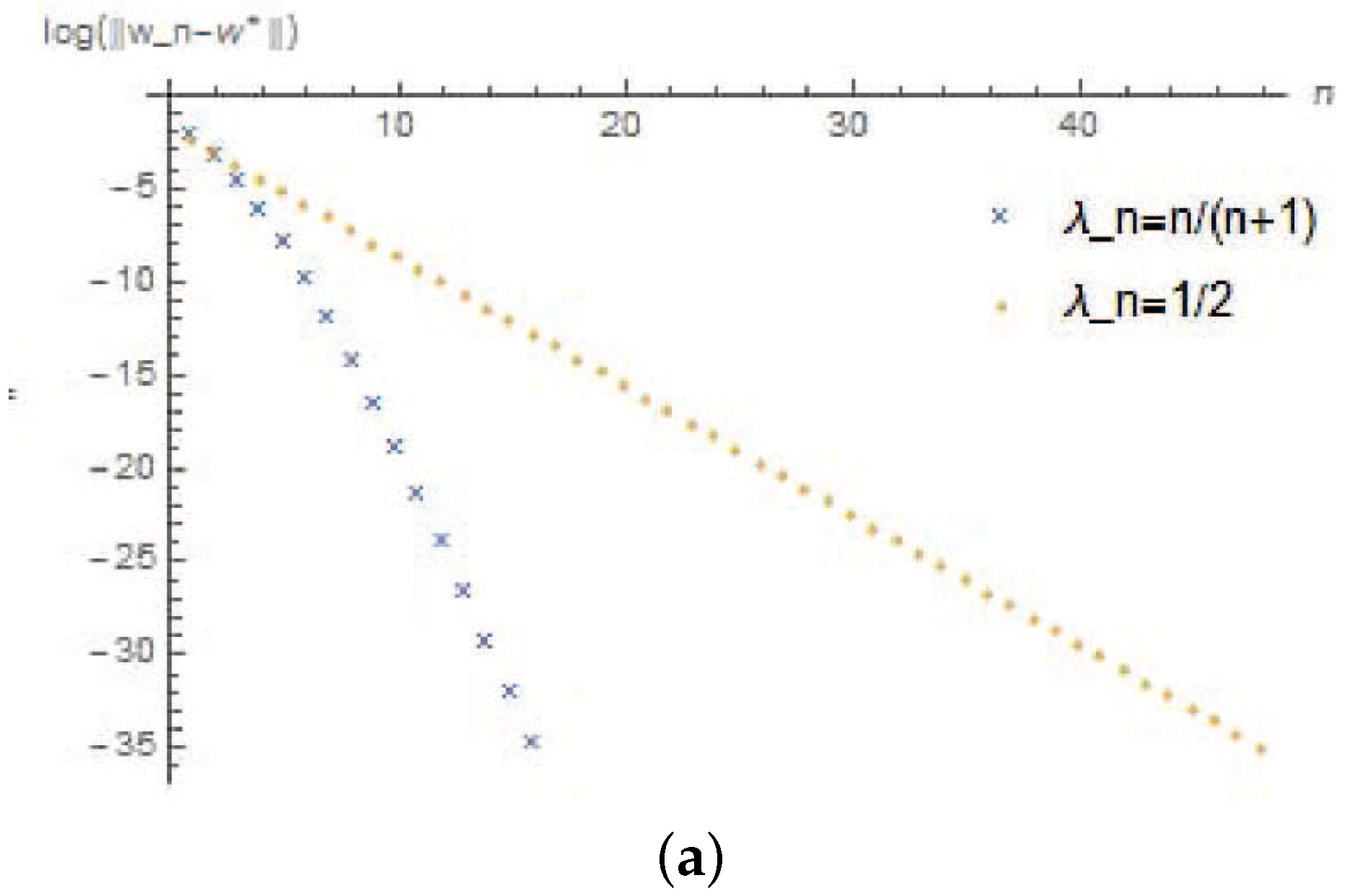
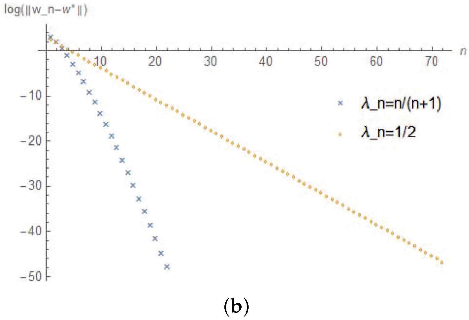
x n + 1 = ( 1 γ n ) x n + γ n z n , y n + 1 = ( 1 γ n ) y n , z n + 1 = ( 1 γ n ) z n + γ n x n .
In algorithm (16), we take γ n = 1 2 , n n + 1 , respectively. Then we have the following numerical results (the x-coordinate denotes the iteration times, and the y-coordinate denotes the logarithm of the error). The whole program was written in Wolfram Mathematica (version 10.3). All the numerical results were performed on a personal Dell computer with Inter(R) Core(TM) i5-7200 U CPU 2.50 GHz and RAM 4.00 GB.
We choose error to be 10 15 , the initial value w 0 = ( 0.5 , 0.2 , 0.4 ) and w 0 = ( 0.8 , 0.8 , 0.5 ) , according to the algorithm (16), they converges to w * = ( 0.45 , 0 , 0.45 ) Γ and w * = ( 0.65 , 0 , 0.65 ) Γ , respectively (See Figure 1).

Author Contributions

Y.J., R.C. and L.S. contributed equally to this work. All authors have read and agreed to the published version of the manuscript.

Funding

This research was funded by NSFC Grants No:11226125; No:11301379.

Conflicts of Interest

The authors declare no conflict of interest.

References

  1. Moudafi, A. A relaxed alternating CQ-algorithm for convex feasibility. Nonlinear Anal. Theory Methods Appl. 2013, 79, 117–121. [Google Scholar] [CrossRef]
  2. Censor, Y. A multiprojection algorithm using Bregman projections in a product space. Numer. Algorithms 1994, 8, 221–239. [Google Scholar] [CrossRef]
  3. Byrne, C. A unified treatment of some iterative algorithms in signal processing and image reconstruction. Inverse Probl. 2004, 20, 103–120. [Google Scholar] [CrossRef] [Green Version]
  4. Censor, Y.; Bortfeld, T.; Martin, B.; Trofimov, A. A unified approach for inversion problems in intensity-modulated radiation therapy. Phys. Med. Biol. 2006, 51, 2353–2365. [Google Scholar] [CrossRef] [Green Version]
  5. Attouch, H.; Cabot, A.; Frankel, F.; Peypouquet, J. Alternating proximal algorithms for linearly constrained variational inequalities. Application to domain decomposition for PDE’s. Nonlinear Anal. 2011, 74, 7455–7473. [Google Scholar] [CrossRef]
  6. Attouch, H.; Bolte, J.; Redont, P.; Soubeyran, A. Alternating proximal algorithms for weakly coupled minimization problems. Applications to dynamical games and PDE’s. J. Convex Anal. 2008, 28, 39–44. [Google Scholar]
  7. Moudafi, A. Alternating CQ-algorithm for convex feasibility and split fixed-point problems. J. Nonlinear Convex Anal. 2014, 15, 809–818. [Google Scholar]
  8. Chen, R.D. Fixed Point Theory and Aplications; National Defense Industry Press: Beijing, China, 2012. [Google Scholar]
  9. Byrne, C.; Censor, Y.; Gibali, A.; Reich, S. The split common null point problem. J. Nonlinear Convex Anal. 2011, 13, 759–775. [Google Scholar]
  10. Eslamian, M.; Shehu, Y.; Iyiola, O.S. A strong convergence theorem for a general split equality problem with applications to optimization and equilibrium problem. Calcolo 2018, 55, 4. [Google Scholar] [CrossRef]
  11. Shi, L.Y.; Ansari, Q.H.; Yao, J.C. Linear convergence of gradient projection algorithm for split equality problems. Optimization 2018, 67, 2347–2358. [Google Scholar] [CrossRef]
  12. Chuang, C.-S. Strong convergence theorems for the split variational inclusion problem in Hilbert spaces. Fixed Point Theory Appl. 2013. [Google Scholar] [CrossRef] [Green Version]
  13. Zhao, X.; Ng, K.F.; Li, C. Linear regularity and linear convergence of projection-based methods for solving convex feasibility problems. Appl. Math. Optim. 2017, 78, 613–641. [Google Scholar] [CrossRef]
  14. Borwein, B.J.M. On projection algorithms for solving convex feasibility problems. Siam Rev. 1996, 38, 367–426. [Google Scholar]
  15. Conway, J.B. A Course in Functional Analysis, 2nd ed.; GTM 96; Springer: Berlin/Heidelberg, Germany, 1989. [Google Scholar]
  16. Zegeye, H.; Shahzad, N. Convergence of Mann’s type iteration method for generalized asymptotically nonexpansive mappings. Comput. Math. Appl. 2011, 62, 4007–4014. [Google Scholar] [CrossRef] [Green Version]
Figure 1. Numerical Results. (a) error = 10−15, w0 = (0.5,0.2,0.4),w* = (0.45,0,0.45), (b) error = 10−15, w0 = (0.8,0.8,0.5),w* = (0.65,0,0.65).
Mathematics 08 01836 g001aMathematics 08 01836 g001b
Publisher’s Note: MDPI stays neutral with regard to jurisdictional claims in published maps and institutional affiliations.

