Particle Swarm Optimization for Predicting the Development Effort of Software Projects


Abstract
1. Introduction
2. Related Work
- (a)
- An increase in the computational cost inherent to CBR models by incorporating the use of optimization techniques.
- (b)
- Allowing selecting the best SDEP model from a set of predefined models, but without an automatically adjustment of the parameters of the selected model.
- (c)
- Define a priori the SDEP model to be used, and only adjusting its parameters.
- (1)
- The selection of the SDEP model, and
- (2)
- The automatic adjustment of the SDEP model parameters.
3. Particle Swarm Optimization (PSO) and PSO-SRE
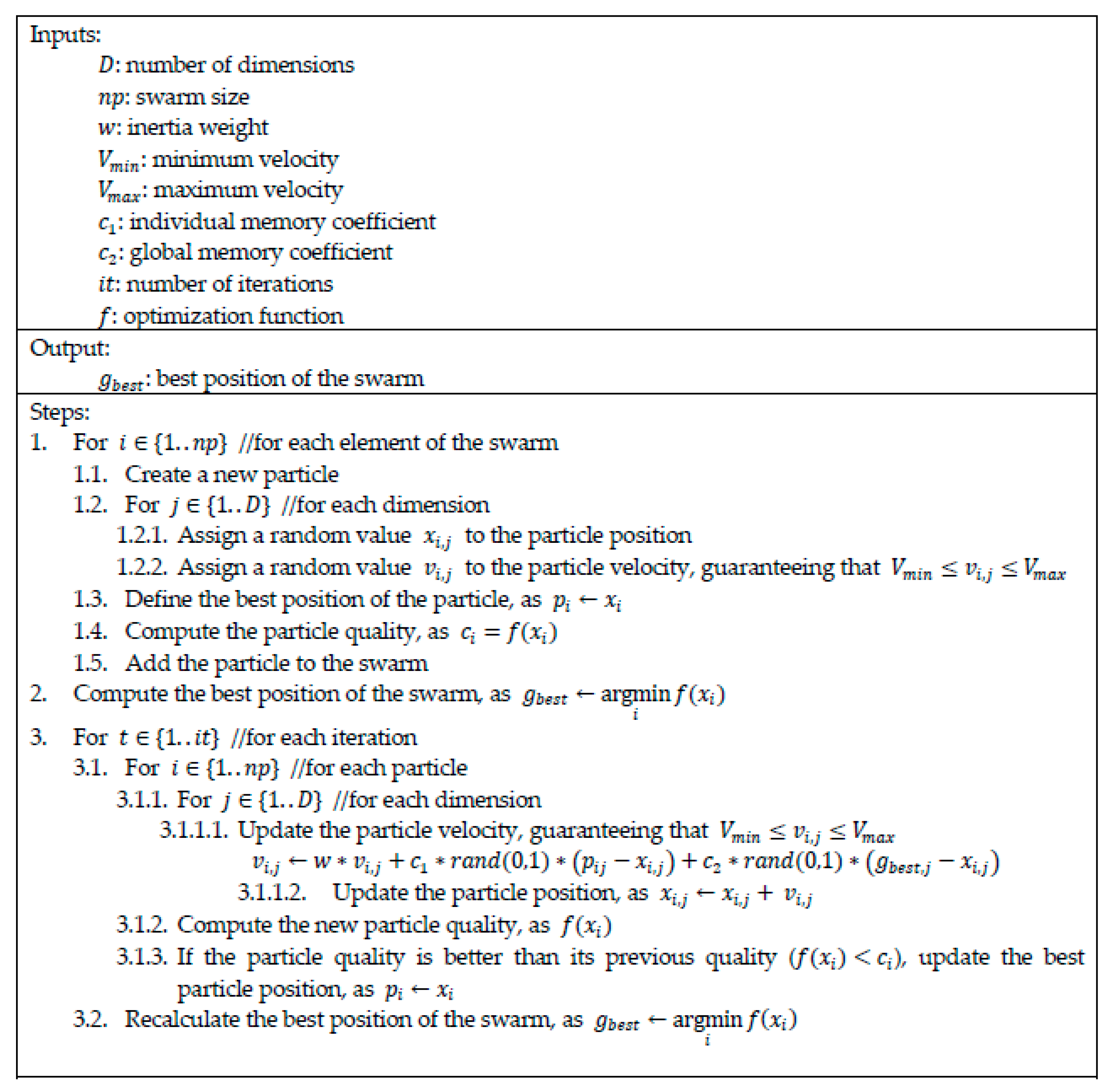
3.1. PSO
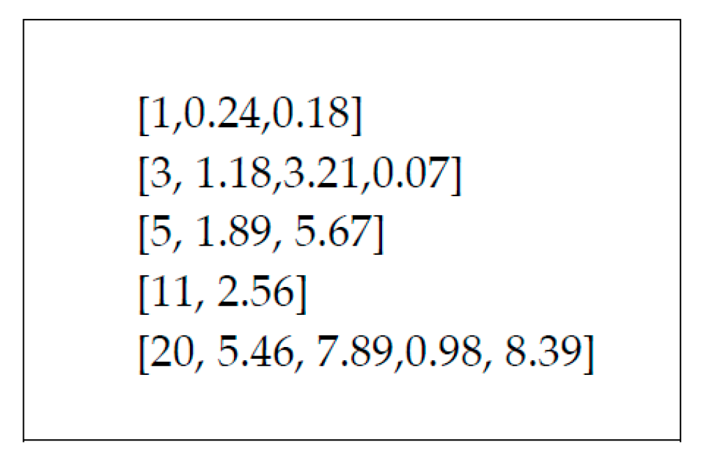
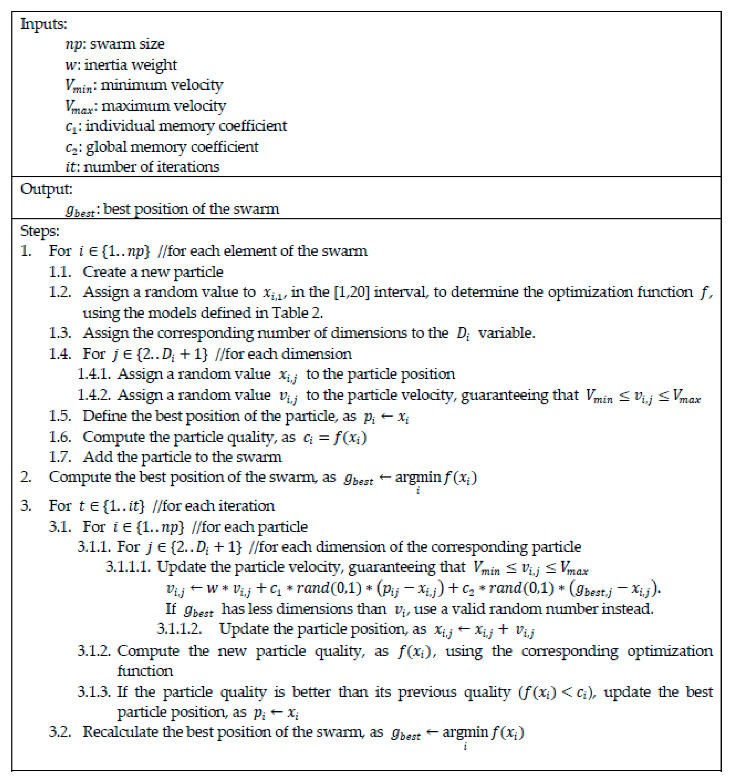
3.2. PSO-SRE
4. Data Sets of Software Projects
5. Results
- Test 1: Up to 500 iterations, and up to 250 individuals in the swarm;
- Test 2: Up to 1500 iterations, and up to 750 individuals in the swarm;
- Test 3: Up to 1000 iterations, and up to 500 individuals in the swarm.
- not have memory of its own nor a search direction,
- repeat the random search of “the best particle” for a number of times that is equal to the number of fitness evaluations in the proposed PSO-SRE,
- compare its best solution with the best solution yielded by PSO-SRE.
6. Conclusions
- (a)
- New software projects coded in 3GL and developed in either Mainframe or Multiplatform and coded in 4GL and developed in Multiplatform.
- (b)
- Software enhancement projects coded in 3GL and developed in Multiplatform, MidRange or personal computer, as well as in those projects coded in 4GL and developed in Multiplatform.
- (c)
- Since the performance of the PSO-SRE resulted statistically equal than SRE, a software manager could also apply PSO-SRE as alternative to an SRE to software enhancement projects coded in 3GL and developed in Mainframe.
7. Discussion
- None of them generate their models by using a recent repository of software projects.
- Regarding the four studies where the ISBSG is used (1) their releases correspond to those published in the years 2007 and 2009, (2) all of them only select one data set from the ISBSG whose sizes are between 134 and 505, and (3) none of them take into account the version of the FSM to select the data set; whereas in our study, (1) the ISBSG release 2018 was used, (2) eight data sets containing between 53 and 440 projects were selected, and (3) all of them took into account the guidelines suggested by the ISBSG, including the type of FSM, that is, our data sets did not mix IFPUG V4 type with V4 and post V4 one.
- The majority of them base their conclusions on a biased prediction accuracy measure, and on a nondeterministic validation method.
- The half of them bases their conclusions on statistically significance.
- (1)
- The use of PSO incorporating an additional component by allowing automatic completion, in a single step, of the selection of the SDEP model, and automatic adjustment of the parameters of the SDEP model.
- (2)
- New and enhancement software projects obtained from the ISBSG release 2018.
- (3)
- Software projects selected taking into account the TD, DP, PLT, and FSM as suggested by the ISBSG.
- (4)
- Preprocessing of data sets through outliers’ analysis, and correlation and determination coefficients.
- (5)
- A nonbiased prediction accuracy measure (i.e., AR) to compare the performance between PSO-SRE and SRE models.
- (6)
- The use of a deterministic validation method for training and testing the models (i.e., LOOCV)
- (7)
- Selection of a suitable statistical test based on number of data sets to be compared, data dependence, and data distribution for comparing the prediction accuracy between PSO-SRE and SRE by data set.
- (8)
- Hypotheses tested from statistically significance.
Author Contributions
Funding
Acknowledgments
Conflicts of Interest
Abbreviations
| 2GL | Programming languages of second generation |
| 3GL | Programming languages of third generation |
| 4GL | Programming languages of fourth generation |
| ABC | Artificial bee colony |
| AFP | Adjusted function points |
| ApG | Application generator |
| AR | Absolute residual |
| CBR | Case-based reasoning |
| COCOMO | Constructive cost model |
| DP | Development platform |
| FSM | Functional sizing method |
| GA | Genetic algorithm |
| IFPUG | International Function Point Users Group |
| ISBSG | International Software Benchmarking Standards Group |
| LOOCV | Leave one-out cross validation |
| MAR | Mean absolute residuals |
| MdAR | Median of absolute residuals |
| MF | Mainframe |
| ML | Machine learning |
| MR | Midrange |
| Multi | Multiplatform |
| PC | Personal computer |
| PLT | Programming language type |
| PSO | Particle swarm optimization |
| PSO-SRE | SRE optimized by means of PSO |
| SDEP | Software development effort prediction |
| SRE | Statistical regression equation |
| TD | Type of development |
References
- Bourque, P.; Fairley, R. Guide to the Software Engineering Body of Knowledge, SWEBOK V3.0; IEEE Computer Society: Washington, DC, USA, 2014. [Google Scholar]
- Wilkie, F.G.; McChesney, I.R.; Morrowa, P.; Tuxworth, C.; Lester, N.G. The value of software sizing. Inf. Softw. Technol. 2011, 53, 1236–1249. [Google Scholar] [CrossRef]
- Gautam, S.S.; Singh, V. The state-of-the-art in software development effort estimation. J. Softw. Evol. Process 2018, 30, e1983. [Google Scholar] [CrossRef]
- Pospieszny, P.; Czarnacka-Chrobot, B.; Kobylinski, A. An effective approach for software project effort and duration estimation with machine learning algorithms. J. Syst. Softw. 2018, 137, 184–196. [Google Scholar] [CrossRef]
- Li, Z.; Jing, X.-Y.; Zhu, X. Progress on approaches to software defect prediction. IET Softw. 2018, 12, 161–175. [Google Scholar] [CrossRef]
- Jorgensen, M.; Shepperd, M. A Systematic Review of Software Development Cost Estimation Studies. IEEE Trans. Softw. Eng. 2007, 33, 33–53. [Google Scholar] [CrossRef]
- Boehm, B.; Abts, C.; Brown, A.W.; Chulani, S.; Clark, B.K.; Horowitz, E.; Madachy, R.; Reifer, D.J.; Steece, B. Software Cost Estimation with COCOMO II; Prentice Hall: Upper Saddle River, NY, USA, 2000. [Google Scholar]
- Ahsan, K.; Gunawan, I. Analysis of cost and schedule performance of international development projects. Int. J. Proj. Manag. 2010, 28, 68–78. [Google Scholar] [CrossRef]
- Doloi, H.K. Understanding stakeholders’ perspective of cost estimation in project management. Int. J. Proj. Manag. 2011, 29, 622–636. [Google Scholar] [CrossRef]
- Jørgensen, M. The effects of the format of software project bidding processes. Int. J. Proj. Manag. 2006, 24, 522–528. [Google Scholar] [CrossRef]
- Savolainen, P.; Ahonen, J.J.; Richardson, I. Software development project success and failure from the supplier’s perspective: A systematic literature review. Int. J. Proj. Manag. 2012, 30, 458–469. [Google Scholar] [CrossRef]
- Carbonera, C.E.; Farias, K.; Bischoff, V. Software development effort estimation: A systematic mapping study. IET Softw. 2020, 14, 328–344. [Google Scholar] [CrossRef]
- López-Martín, C. Predictive Accuracy Comparison between Neural Networks and Statistical Regression for Development Effort of Software Projects. Appl. Soft Comput. 2015, 27, 434–449. [Google Scholar] [CrossRef]
- Chavoya, A.; López-Martín, C.; Andalon-Garcia, I.R.; Meda-Campaña, M.E. Genetic programming as alternative for predicting development effort of individual software projects. PLoS ONE 2012, 7, e50531. [Google Scholar] [CrossRef] [PubMed][Green Version]
- Wang, D.; Tan, D.; Liu, L. Particle swarm optimization algorithm: An overview. Soft Comput. 2018, 22, 387–408. [Google Scholar] [CrossRef]
- Yeoh, J.M.; Caraffini, F.; Homapour, E.; Santucci, V.; Milani, A. A Clustering System for Dynamic Data Streams Based on Metaheuristic Optimisation. Mathematics 2019, 7, 1229. [Google Scholar] [CrossRef]
- Kim, M.; Chae, J. Monarch Butterfly Optimization for Facility Layout Design Based on a Single Loop Material Handling Path. Mathematics 2019, 7, 154. [Google Scholar] [CrossRef]
- García, J.; Yepes, V.; Martí, J.V. A Hybrid k-Means Cuckoo Search Algorithm Applied to the Counterfort Retaining Walls Problem. Mathematics 2020, 8, 555. [Google Scholar] [CrossRef]
- Li, J.; Guo, L.; Li, Y.; Liu, C. Enhancing Elephant Herding Optimization with Novel Individual Updating Strategies for Large-Scale Optimization Problems. Mathematics 2019, 7, 395. [Google Scholar] [CrossRef]
- Balande, U.; Shrimankar, D. SRIFA: Stochastic Ranking with Improved-Firefly-Algorithm for Constrained Optimization Engineering Design Problems. Mathematics 2019, 7, 250. [Google Scholar] [CrossRef]
- Feng, Y.; An, H.; Gao, X. The Importance of Transfer Function in Solving Set-Union Knapsack Problem Based on Discrete Moth Search Algorithm. Mathematics 2019, 7, 17. [Google Scholar] [CrossRef]
- Shih, P.-C.; Chiu, C.-Y.; Chou, C.-H. Using Dynamic Adjusting NGHS-ANN for Predicting the Recidivism Rate of Commuted Prisoners. Mathematics 2019, 7, 1187. [Google Scholar] [CrossRef]
- Grigoraș, G.; Neagu, B.-C.; Gavrilaș, M.; Triștiu, I.; Bulac, C. Optimal Phase Load Balancing in Low Voltage Distribution Networks Using a Smart Meter Data-Based Algorithm. Mathematics 2020, 8, 549. [Google Scholar] [CrossRef]
- Jouhari, H.; Lei, D.; A. A. Al-qaness, M.; Abd Elaziz, M.; Ewees, A.A.; Farouk, O. Sine-Cosine Algorithm to Enhance Simulated Annealing for Unrelated Parallel Machine Scheduling with Setup Times. Mathematics 2019, 7, 1120. [Google Scholar] [CrossRef]
- Khuat, T.T.; Le, M.H. A Novel Hybrid ABC-PSO Algorithm for Effort Estimation of Software Projects Using Agile Methodologies. J. Intell. Syst. 2018, 27, 489–506. [Google Scholar] [CrossRef]
- Srivastava, P.R.; Varshney, A.; Nama, P.; Yang, X.-S. Software test effort estimation: A model based on cuckoo search. Int. J. Bio-Inspired Comput. 2012, 4, 278–285. [Google Scholar] [CrossRef]
- Benala, T.R.; Mall, R. DABE: Differential evolution in analogy-based software development effort estimation. Swarm Evol. Comput. 2018, 38, 158–172. [Google Scholar] [CrossRef]
- Huang, S.J.; Chiu, N.H.; Chen, L.W. Integration of the grey relational analysis with genetic algorithm for software effort estimation. Eur. J. Oper. Res. 2008, 188, 898–909. [Google Scholar] [CrossRef]
- Chhabra, S.; Singh, H. Optimizing Design of Fuzzy Model for Software Cost Estimation Using Particle Swarm Optimization Algorithm. Int. J. Comput. Intell. Appl. 2020, 19, 2050005. [Google Scholar] [CrossRef]
- Uysal, M. Using heuristic search algorithms for predicting the effort of software projects. Appl. Comput. Math. 2009, 8, 251–262. [Google Scholar]
- Kaushik, A.; Tayal, D.K.; Yadav, K. The Role of Neural Networks and Metaheuristics in Agile Software Development Effort Estimation. Int. J. Inf. Technol. Proj. Manag. 2020, 11. [Google Scholar] [CrossRef]
- Zare, F.; Zare, H.K.; Fallahnezhad, M.S. Software effort estimation based on the optimal Bayesian belief network. Appl. Soft Comput. 2016, 49, 968–980. [Google Scholar] [CrossRef]
- Azzeh, M.; Bou-Nassif, A.; Banitaan, S.; Almasalha, F. Pareto efficient multi-objective optimization for local tuning of analogy-based estimation. Neural Comput. Appl. 2016, 27, 2241–2265. [Google Scholar] [CrossRef]
- Bardsiri, V.K.; Jawawi, D.N.A.; Hashim, S.Z.M.; Khatibi, E. A PSO-based model to increase the accuracy of software development effort estimation. Softw. Qual. J. 2013, 21, 501–526. [Google Scholar] [CrossRef]
- Bardsiri, V.K.; Jawawi, D.N.A.; Hashim, S.Z.M.; Khatibi, E. A flexible method to estimate the software development effort based on the classification of projects and localization of comparisons. Emp. Softw. Eng. 2014, 19, 857–884. [Google Scholar] [CrossRef]
- Wu, D.; Li, J.; Bao, C. Case-based reasoning with optimized weight derived by particle swarm optimization for software effort estimation. Soft Comput. 2018, 22, 5299–5310. [Google Scholar] [CrossRef]
- Wu, D.; Li, J.; Liang, Y. Linear combination of multiple case-based reasoning with optimized weight for software effort estimation. J. Supercomput. 2013, 64, 898–918. [Google Scholar] [CrossRef]
- Sheta, A.F.; Ayesh, A.; Rine, D. Evaluating software cost estimation models using particle swarm optimisation and fuzzy logic for NASA projects: A comparative study. Int. J. Bio-Inspired Comput. 2010, 2. [Google Scholar] [CrossRef]
- Bohem, B. Software Engineering Economics; Prentice Hall: Upper Saddle River, NJ, USA, 1981. [Google Scholar]
- Hosni, M.; Idri, A.; Abran, A.; Bou-Nassif, A. On the value of parameter tuning in heterogeneous ensembles effort estimation. Soft Comput. 2018, 22, 5977–6010. [Google Scholar] [CrossRef]
- ISBSG. Guidelines for Use of the ISBSG Data Release 2018; International Software Benchmarking Standards Group: Melbourne, Australia, 2018. [Google Scholar]
- González-Ladrón-de-Guevara, F.; Fernández-Diego, M.; Lokan, C. The usage of ISBSG data fields in software effort estimation: A systematic mapping study. J. Syst. Softw. 2016, 113, 188–215. [Google Scholar] [CrossRef]
- Kitchenham, B.; Mendes, E. Why comparative effort prediction studies may be invalid. In Proceedings of the 5th International Conference on Predictor Models in Software Engineering (PROMISE), Vancouver, BC, Canada, 18–19 May 2009. [Google Scholar] [CrossRef]
- Ali, A.; Gravino, C. A systematic literature review of software effort prediction using machine learning methods. J. Softw. Evol. Process 2019, 31, e2211. [Google Scholar] [CrossRef]
- Wen, J.; Li, S.; Lin, Z.; Hu, Y.; Huang, C. Systematic literature review of machine learning based software development effort estimation models. Inf. Softw. Technol. 2012, 54, 41–59. [Google Scholar] [CrossRef]
- Dybå, T.; Kampenes, V.B.; Sjøberg, D.I.K. A systematic review of statistical power in software engineering experiments. J. Inf. Softw. Technol. 2006, 48, 745–755. [Google Scholar] [CrossRef]
- Kocaguneli, E.; Menzies, T. Software effort models should be assessed via leave- one-out validation. J. Syst. Softw. 2013, 86, 1879–1890. [Google Scholar] [CrossRef]
- Mahmood, Y.; Kama, N.; Azmi, A. A systematic review of studies on use case points and expert-based estimation of software development effort. J. Softw. Evol. Process 2020, e2245. [Google Scholar] [CrossRef]
- Idri, A.; Hosni, M.; Abran, A. Systematic literature review of ensemble effort estimation. J. Syst. Softw. 2016, 118, 151–175. [Google Scholar] [CrossRef]
- Idri, A.; Amazal, F.A.; Abran, A. Analogy-based software development effort estimation: A systematic mapping and review. Inf. Softw. Technol. 2015, 58, 206–230. [Google Scholar] [CrossRef]
- Afzal, W.; Torkar, R. On the application of genetic programming for software engineering predictive modeling: A systematic review. Expert Syst. Appl. 2011, 38, 11984–11997. [Google Scholar] [CrossRef]
- Halkjelsvik, T.; Jørgensen, M. From origami to software development: A review of studies on judgment-based predictions of performance time. Psychol. Bull. 2012, 138, 238–271. [Google Scholar] [CrossRef]
- Yang, Y.; He, Z.; Mao, K.; Li, Q.; Nguyen, V.; Boehm, B.; Valerdi, R. Analyzing and handling local bias for calibrating parametric cost estimation models. Inf. Softw. Technol. 2013, 55, 1496–1511. [Google Scholar] [CrossRef]
- Kennedy, J.; Eberhart, R. Particle Swarm Optimization. In Proceedings of the 1995 International Conference on Neural Networks, Perth, Australia, 27 November–1 December 1995; Volume 4, pp. 1942–1948. [Google Scholar]
- Shi, Y.; Eberhart, R.C. A Modified Particle Swarm Optimizer. In Proceedings of the IEEE International Conference on Evolutionary Computation, Anchorage, AK, USA, 4–9 May 1998. [Google Scholar]
- Onofri, A. Nonlinear Regression Analysis: A Tutorial. Available online: https://www.statforbiology.com/nonlinearregression/usefulequations#logistic_curve (accessed on 29 July 2020).
- Billo, E.J. Excel for Scientists and Engineers: Numerical Methods; John Wiley & Sons: New York, NY, USA, 2007; Available online: https://onlinelibrary.wiley.com/doi/pdf/10.1002/9780470126714.app4#:~:text=The%20curve%20follows%20equation%20A42,%2B%20ex2%20%2Bfx%20%2B%20g (accessed on 30 July 2020).
- Sherrod, P.H. Nonlinear Regression Analysis Program. Nashville, TN, USA 2005. Available online: http://curve-fitting.com/asymptot.htm (accessed on 30 July 2020).
- ISBSG. ISBSG Demographics, International Software Benchmarking Standards Group; International Software Benchmarking Standards Group: Melbourne, Australia, 2018. [Google Scholar]
- Fox, J.P. Bayesian Item Response Modeling, Theory and Applications. Stat. Soc. Behav. Sci. 2010. [Google Scholar] [CrossRef]
- Humphrey, W.S. A Discipline for Software Engineering, 1st ed.; Addison-Wesley: Boston, MA, USA, 1995. [Google Scholar]
- Barrera, J.; Álvarez-Bajo, O.; Flores, J.J.; Coello Coello, C.A. Limiting the velocity in the particle swarm optimization algorithm. Comput. Sist. 2016, 20, 635–645. [Google Scholar] [CrossRef][Green Version]
- Moore, D.S.; McCabe, G.P.; Craig, B.A. Introduction to the Practice of Statistics, 6th ed.; W.H. Freeman and Company: New York, NY, USA, 2009. [Google Scholar]
- López-Yáñez, I.; Argüelles-Cruz, A.J.; Camacho-Nieto, O.; Yáñez-Márquez, C. Pollutants time series prediction using the Gamma classifier. Int. J. Comput. Intell. Syst. 2011, 4, 680–711. [Google Scholar] [CrossRef]
- Uriarte-Arcia, A.V.; Yáñez-Márquez, C.; Gama, J.; López-Yáñez, I.; Camacho-Nieto, O. Data Stream Classification Based on the Gamma Classifier. Math. Probl. Eng. 2015, 2015, 939175. [Google Scholar] [CrossRef]
- Shepperd, M.; MacDonell, S. Evaluating prediction systems in software project estimation. Inf. Softw. Technol. 2012, 54, 820–827. [Google Scholar] [CrossRef]


| Study | Data Set(s) 1 | Prediction Accuracy | Validation Method | Statistical Significance? |
|---|---|---|---|---|
| [25] | Six software organizations (21) | AR MRE r2 | NS | Wilcoxon |
| [33] | Albrecht (24) Kemerer (15) Nasa (18) ISBSG Release 10 (505) Desharnais (77) Desharnais L1 (44) 3 Desharnais L2 (23) Desharnais L3 (10) Cocomo (63) Cocomo E (28) Cocomo O (24) Cocomo S (11) China (499) Maxwell (62) Telecom (18) | BRE IBRE | LOOCV | ANOVA |
| [34] | Canadian organization (21) IBM (24) ISBSG Release 11 (134) | MRE | k-fold cross validation (k = 3) | No |
| [35] | ISBSG Release 2011 (380) Cocomo (63) Maxwell (62) | MRE | k-fold cross validation (k = 10) | Wilcoxon |
| [29] | Cocomo NASA 2 (93) Cocomo (60) | MRE | NS | No |
| [40] | Albrecht (24) China (499) COCOMO (252) 2 Desharnais (77) ISBSG Release 8, 2003 (148) Kemerer (15) Miyazaki (48) | AR MRE LSD BRE IBRE | LOOCV | Scott-Knott |
| [38] | Nasa (18) | MRE | Hold-out | No |
| [36] | Desharnais (77) Maxwell (62) | MRE | k-fold cross validation (k = 3) | No |
| [37] | Desharnais (77) Miyazaki (48) | MRE | k-fold cross validation (k = 3) | t-Student |
| [32] | Cocomo (63) | MRE | Hold-out | No |
| No. | Model | Equation | Reference |
|---|---|---|---|
| 1 | Linear equation | [56] | |
| 2 | Exponential equation | [56] | |
| 3 | Exponential decrease or increase between limits | [57] | |
| 4 | Double exponential decay to zero | [57] | |
| 5 | Power | [57] | |
| 6 | Asymptotic equation | [58] | |
| 7 | Asymptotic regression model | [56] | |
| 8 | Logarithmic | [57] | |
| 9 | “Plateau” curve—Michaelis-Menten equation | [57] | |
| 10 | Yield-loss/density curves | [54] | |
| 11 | Logistic Function | [57] | |
| 12 | Logistic curves with additional parameters | [57] | |
| 13 | Logistic curve with offset on the y-Axis | [57] | |
| 14 | Gaussian curve | [57] | |
| 15 | Log vs. Reciprocal | [57] | |
| 16 | Trigonometric functions | [57] | |
| 17 | Trigonometric functions (2) | [57] | |
| 18 | Trigonometric functions (3) | [57] | |
| 19 | Quadratic polynomial regression | [57] | |
| 20 | Cubic polynomial regression | [57] |
| Attribute | Selected Value(s) | Projects |
|---|---|---|
| Adjusted Function Point not null | --- | 6394 |
| Data quality rating | A, B | 6061 |
| Unadjusted Function Point Rating | A, B | 5316 |
| Functional sizing methods | IFPUG 4+ | 4602 |
| Development platform not null | --- | 3040 |
| Language type not null | --- | 2711 |
| Resource level | 1 | 2054 |
| TD | DP | PLT | NSP |
|---|---|---|---|
| New | MF | 2GL | 3 |
| MF | 3GL | 133 | |
| MF | 4GL | 28 | |
| MF | ApG | 4 | |
| MR | 3GL | 36 | |
| MR | 4GL | 22 | |
| Multi | 3GL | 105 | |
| Multi | 4GL | 102 | |
| PC | 3GL | 55 | |
| PC | 4GL | 118 | |
| Proprietary | 5GL | 12 | |
| Enhancement | MF | 2GL | 4 |
| MF | 3GL | 457 | |
| MF | 4GL | 48 | |
| MF | ApG | 53 | |
| MR | 3GL | 67 | |
| MR | 4GL | 53 | |
| Multi | 3GL | 442 | |
| Multi | 4GL | 195 | |
| PC | 3GL | 55 | |
| PC | 4GL | 42 |
| TD | DP | PLT | NSP | Variable | Normality Test | |||
|---|---|---|---|---|---|---|---|---|
| χ2 | S-W | Skewness | Kurtosis | |||||
| New | MF | 3GL | 133 | AFP | 0.0000 | 0.0000 | 0.0000 | 0.0000 |
| Effort | 0.0000 | 0.0000 | 0.0000 | 0.0000 | ||||
| MR | 3GL | 36 | AFP | 0.0354 | 0.0075 | 0.1836 | 0.8342 | |
| Effort | 0.0000 | 0.0000 | 0.0000 | 0.0000 | ||||
| Multi | 3GL | 105 | AFP | 0.0000 | 0.0000 | 0.0000 | 0.0000 | |
| Effort | 0.0000 | 0.0000 | 0.0000 | 0.0000 | ||||
| Multi | 4GL | 102 | AFP | 0.0000 | 0.0000 | 0.0000 | 0.0000 | |
| Effort | 0.0000 | 0.0000 | 0.0000 | 0.0000 | ||||
| PC | 3GL | 55 | AFP | 0.0000 | 0.0000 | 0.0000 | 0.0000 | |
| Effort | 0.0000 | 0.0000 | 0.0000 | 0.0000 | ||||
| PC | 4GL | 118 | AFP | 0.0000 | 0.0000 | 0.0002 | 0.0158 | |
| Effort | 0.0000 | 0.0000 | 0.0000 | 0.0000 | ||||
| Enhancement | MF | 3GL | 457 | AFP | 0.0000 | 0.0000 | 0.0000 | 0.0000 |
| Effort | 0.0000 | 0.0000 | 0.0000 | 0.0000 | ||||
| MF | 4GL | 48 | AFP | 0.0000 | 0.0000 | 0.0000 | 0.0000 | |
| Effort | 0.0186 | 0.0000 | 0.0104 | 0.0300 | ||||
| MF | ApG | 53 | AFP | 0.0000 | 0.0000 | 0.0000 | 0.0000 | |
| Effort | 0.0000 | 0.0000 | 0.0002 | 0.0000 | ||||
| MR | 3GL | 67 | AFP | 0.0000 | 0.0000 | 0.0000 | 0.0000 | |
| Effort | 0.0000 | 0.0000 | 0.0000 | 0.0000 | ||||
| MR | 4GL | 53 | AFP | 0.0000 | 0.0000 | 0.0117 | 0.1535 | |
| Effort | 0.0000 | 0.0000 | 0.0001 | 0.0000 | ||||
| Multi | 3GL | 442 | AFP | 0.0000 | 0.0000 | 0.0000 | 0.0000 | |
| Effort | 0.0000 | 0.0000 | 0.0000 | 0.0000 | ||||
| Multi | 4GL | 195 | AFP | 0.0000 | 0.0000 | 0.0000 | 0.0000 | |
| Effort | 0.0000 | 0.0000 | 0.0000 | 0.0000 | ||||
| PC | 3GL | 55 | AFP | 0.0000 | 0.0000 | 0.0003 | 0.0003 | |
| Effort | 0.0000 | 0.0000 | 0.0000 | 0.0000 | ||||
| PC | 4GL | 42 | AFP | 0.0000 | 0.0000 | 0.0006 | 0.0001 | |
| Effort | 0.0203 | 0.0000 | 0.0047 | 0.0006 | ||||
| TD | DP | LT | NSP | NO | FDSS | % | r | r2 |
|---|---|---|---|---|---|---|---|---|
| New | MF | 3GL | 133 | 3 | 130 | 2.25 | 0.7345 | 0.5396 |
| MR | 3GL | 36 | 6 | 30 | 16.6 | 0.7390 | 0.5461 | |
| Multi | 3GL | 105 | 6 | 99 | 5.71 | 0.7227 | 0.5223 | |
| Multi | 4GL | 102 | 6 | 96 | 5.88 | 0.8513 | 0.7247 | |
| PC | 3GL | 55 | 7 | 48 | 12.72 | 0.7978 | 0.6365 | |
| PC | 4GL | 118 | 6 | 112 | 5.08 | 0.6515 | 0.4245 | |
| Enhancement | MF | 3GL | 457 | 17 | 440 | 3.86 | 0.7916 | 0.6266 |
| MF | 4GL | 48 | 4 | 44 | 9.09 | 0.4751 | 0.2257 | |
| MF | ApG | 53 | 4 | 49 | 8.16 | 0.6571 | 0.4318 | |
| MR | 3GL | 67 | 3 | 64 | 4.68 | 0.8052 | 0.6483 | |
| MR | 4GL | 53 | 6 | 47 | 11.32 | 0.7127 | 0.5080 | |
| Multi | 3GL | 442 | 14 | 428 | 3.16 | 0.8016 | 0.6427 | |
| Multi | 4GL | 195 | 5 | 190 | 2.56 | 0.7640 | 0.5838 | |
| PC | 3GL | 55 | 2 | 53 | 3.77 | 0.8019 | 0.6431 | |
| PC | 4GL | 42 | 6 | 36 | 14.28 | 0.6418 | 0.4119 |
| TD | DP | LT | SRE |
|---|---|---|---|
| New | MF | 3GL | |
| Multi | 3GL | ||
| Multi | 4GL | ||
| Enhancement | MF | 3GL | |
| MR | 3GL | ||
| Multi | 3GL | ||
| Multi | 4GL | ||
| PC | 3GL |
| TD | DP | LT | NSP | ID SRE | Model Name | Test 1 | Test 2 | Test 3 | |||
|---|---|---|---|---|---|---|---|---|---|---|---|
| SS | Iterations | SS | Iterations | SS | Iterations | ||||||
| New | MF | 3GL | 130 | 1 | DEDZ | 50 | 250 | 150 | 750 | 100 | 500 |
| Multi | 3GL | 99 | 2 | LE | 50 | 250 | 150 | 750 | 100 | 500 | |
| Multi | 4GL | 96 | 3 | LE | 50 | 250 | 150 | 750 | 100 | 500 | |
| Enhancement | MF | 3GL | 440 | 4 | LE | 250 | 500 | 750 | 1500 | 500 | 1000 |
| MR | 3GL | 64 | 5 | LE | 50 | 250 | 150 | 750 | 100 | 500 | |
| Multi | 3GL | 428 | 6 | Pcu | 50 | 250 | 150 | 750 | 100 | 500 | |
| Multi | 4GL | 190 | 7 | Pcu | 50 | 250 | 150 | 750 | 100 | 500 | |
| PC | 3GL | 53 | 8 | AE | 50 | 500 | 150 | 1500 | 100 | 1000 | |
| TD | ID SRE | LT | NSP | SRE | RS | PSO-SRE | |||||||
|---|---|---|---|---|---|---|---|---|---|---|---|---|---|
| Test 1 | Test 2 | Test 3 | |||||||||||
| MAR | MdAR | MAR | MdAR | MAR | MdAR | MAR | MdAR | MAR | MdAR | ||||
| New | 1 | 3GL | 130 | 0.66 | 0.60 | 1.73 | 1.83 | 0.54 | 0.41 | 0.61 | 0.51 | 0.61 | 0.51 |
| 2 | 3GL | 99 | 0.62 | 0.56 | 1.46 | 1.35 | 0.56 | 0.43 | 0.61 | 0.55 | 0.61 | 0.55 | |
| 3 | 4GL | 96 | 0.53 | 0.49 | 0.74 | 0.57 | 0.43 | 0.32 | 0.52 | 0.47 | 0.52 | 0.47 | |
| Enhancement | 4 | 3GL | 440 | 0.61 | 0.52 | 1.99 | 2.01 | 0.61 | 0.50 | 0.61 | 0.50 | 0.61 | 0.52 |
| 5 | 3GL | 64 | 0.60 | 0.50 | 1.33 | 1.21 | 0.53 | 0.35 | 0.59 | 0.49 | 0.59 | 0.49 | |
| 6 | 3GL | 428 | 0.56 | 0.50 | 1.62 | 1.60 | 0.40 | 0.28 | 0.55 | 0.48 | 0.54 | 0.46 | |
| 7 | 4GL | 190 | 0.52 | 0.44 | 1.37 | 1.46 | 0.46 | 0.41 | 0.51 | 0.45 | 0.51 | 0.45 | |
| 8 | 3GL | 53 | 0.72 | 0.70 | 1.18 | 1.06 | 0.48 | 0.36 | 0.72 | 0.70 | 0.65 | 0.55 | |
| TD | DP | LT | NSP | Pair | χ2 | S-W | Skewness | Kurtosis | p-Value |
|---|---|---|---|---|---|---|---|---|---|
| New | MF | 3GL | 130 | SRE | 0.0000 | 0.0000 | 0.3410 | 0.0000 | 0.0000 |
| RS | 0.0000 | 0.0000 | 0.0073 | 0.9537 | 0.0000 | ||||
| Multi | 3GL | 99 | SRE | 0.0000 | 0.0000 | 0.0000 | 0.0000 | 0.0040 | |
| RS | 0.1462 | 0.0160 | 0.2573 | 0.6616 | 0.0000 | ||||
| Multi | 4GL | 96 | SRE | 0.0000 | 0.0000 | 0.2251 | 0.0000 | 0.0000 | |
| RS | 0.2261 | 0.0387 | 0.8034 | 0.0428 | 0.0000 | ||||
| Enhancement | MF | 3GL | 440 | SRE | 0.0000 | 0.0000 | 0.6019 | 0.0000 | 0.3878 |
| RS | 0.0000 | 0.0000 | 0.0000 | 0.0014 | 0.0000 | ||||
| MR | 3GL | 64 | SRE | 0.0016 | 0.5511 | 0.7769 | 0.9573 | 0.0267 | |
| RS | 0.7847 | 0.8470 | 0.6219 | 0.9685 | 0.0000 | ||||
| Multi | 3GL | 428 | SRE | 0.0000 | 0.0000 | 0.1028 | 0.0000 | 0.0000 | |
| RS | 0.0000 | 0.0000 | 0.0000 | 0.5221 | 0.0000 | ||||
| Multi | 4GL | 190 | SRE | 0.0000 | 0.0000 | 0.8475 | 0.0000 | 0.0000 | |
| RS | 0.0002 | 0.0000 | 0.0322 | 0.1907 | 0.0000 | ||||
| PC | 3GL | 53 | SRE | 0.0347 | 0.0002 | 0.0961 | 0.0155 | 0.0000 | |
| RS | 0.8419 | 0.2107 | 0.5087 | 0.3184 | 0.0000 |
| TD | DP | LT | NSP | Model Name | Execution Time (Minutes) | |||
|---|---|---|---|---|---|---|---|---|
| Test 1 | Test 2 | Test 3 | Prediction | |||||
| New | MF | 3GL | 130 | Double Exponential Decay to Zero | 14.5 | 23.6 | 36.1 | 0.28 |
| Multi | 3GL | 99 | Linear equation | 10.8 | 19.1 | 30.0 | 0.30 | |
| Multi | 4GL | 96 | Linear equation | 10.7 | 18.9 | 28.9 | 0.30 | |
| Enhancement | MF | 3GL | 440 | Linear equation | 61.6 | 122.2 | 183.6 | 0.42 |
| MR | 3GL | 64 | Linear equation | 7.1 | 14.4 | 17.9 | 0.28 | |
| Multi | 3GL | 428 | “Plateau” curve | 49.8 | 103.8 | 165.1 | 0.39 | |
| Multi | 4GL | 190 | “Plateau” curve | 18.9 | 27.9 | 49.8 | 0.26 | |
| PC | 3GL | 53 | Asymptotic equation | 5.3 | 9.2 | 15.1 | 0.28 | |
Publisher’s Note: MDPI stays neutral with regard to jurisdictional claims in published maps and institutional affiliations. |
© 2020 by the authors. Licensee MDPI, Basel, Switzerland. This article is an open access article distributed under the terms and conditions of the Creative Commons Attribution (CC BY) license (http://creativecommons.org/licenses/by/4.0/).
Share and Cite
Alanis-Tamez, M.D.; López-Martín, C.; Villuendas-Rey, Y. Particle Swarm Optimization for Predicting the Development Effort of Software Projects. Mathematics 2020, 8, 1819. https://doi.org/10.3390/math8101819
Alanis-Tamez MD, López-Martín C, Villuendas-Rey Y. Particle Swarm Optimization for Predicting the Development Effort of Software Projects. Mathematics. 2020; 8(10):1819. https://doi.org/10.3390/math8101819
Chicago/Turabian StyleAlanis-Tamez, Mariana Dayanara, Cuauhtémoc López-Martín, and Yenny Villuendas-Rey. 2020. "Particle Swarm Optimization for Predicting the Development Effort of Software Projects" Mathematics 8, no. 10: 1819. https://doi.org/10.3390/math8101819
APA StyleAlanis-Tamez, M. D., López-Martín, C., & Villuendas-Rey, Y. (2020). Particle Swarm Optimization for Predicting the Development Effort of Software Projects. Mathematics, 8(10), 1819. https://doi.org/10.3390/math8101819