Article

A New Continuous-Discrete Fuzzy Model and Its Application in Finance

1
Division of Computational Mathematics and Engineering, Institute for Computational Science, Ton Duc Thang University, Ho Chi Minh City 70000, Vietnam
2
Faculty of Mathematics and Statistics, Ton Duc Thang University, Ho Chi Minh City 758307, Vietnam
3
Department of Mathematics, College of Science, King Saud University, P.O. Box 2455, Riyadh 11451, Saudi Arabia
4
Departamento de Matemática, Universidad de Tarapacá, Casilla 7D, Arica 09010, Chile
*
Author to whom correspondence should be addressed.
Mathematics 2020, 8(10), 1808; https://doi.org/10.3390/math8101808
Submission received: 19 September 2020 / Revised: 2 October 2020 / Accepted: 5 October 2020 / Published: 16 October 2020
(This article belongs to the Special Issue Fuzzy Sets, Fuzzy Logic and Their Applications 2020)

Abstract

:
In this paper, we propose a fuzzy differential-difference equation for modeling of mixed continuous-discrete phenomena. In the special case, we present the general solution of linear fuzzy differential-difference equations. The dynamical process in the intervals is presented by the corresponding fuzzy differential equation and with impulsive jumps in some points. We illustrate the applicability of the model to study the time value of money.

1. Introduction

Differential and difference equations play a relevant role in modeling problems that arise in physics, engineering, biology, economics, finance, and many other areas. However, in some cases, these equations are restricted in their ability to describe phenomena due to the imprecise or incomplete information about the parameters, variables and initial conditions available. This can result from errors in measurement, observation, or experimental data; application of different operating conditions; or maintenance induced errors [1]. To overcome uncertainties or lack of precision, one can use a fuzzy environment in parameters, variables and initial conditions in place of exact (fixed) ones, by turning general differential and difference equations into fuzzy differential and difference equations, respectively [1,2,3,4,5,6,7]. These uncertainties may be modeled by fuzzy set theory when an abundance of data is not available. Accordingly, there is often a need to model, solve and interpret the problems one encounters in the world of uncertainty. The governing differential and difference equations will then become uncertain. Therefore, recently many researchers have studied fuzzy differential equations and fuzzy difference equations in different approaches [8,9,10,11,12].
Fuzzy set theory refers to the uncertainty when we have a lack of knowledge or incomplete information about the variables and parameters. In the financial markets there are elements of uncertainties and lack of precision associates to fluctuation and votality of financial markets. We cannot make forecasts easily, we have incomplete information or some type of uncertainty, about the values of financial factors such as taxes, inflation, interest rate, price change rate among other factors [4,13,14]. In this direction, some problems of the financial field can be approached via fuzzy difference equations [4]. In particular, Papadopoulos at al. in Reference [4] demonstrated the applicability of fuzzy difference equations to the problems of time value of money. The results obtained in the article [4] were motivated by models introduced by Kwapisz in Reference [15], where several difference equations to study the basic problems of finance such as capital deposits and capital investments were presented.
Although small discrete systems are easy to work with, the continuous models are easier to deal with than large discrete systems. Whether or not nature is fundamentally discrete, the most useful models are often continuous because the discreteness can only occur in very small scales. Discrete models are probably useful if nature has genuinely discrete structure. But on larger scales a discrete model would contain some parameters that we cannot measure and might not even be interested in. This is related to the observation that continuous models often work well for large discrete systems. Discreteness is useful to include in the model if it occurs in the situation we are interested in. Therefore, a mixed continuous-discrete model and, in a special case, a differential-difference equation can possess the inherent properties and advantages of both discrete and continuous models which are useful for modeling of real-world phenomena. In this direction, Kwapisz in Reference [15] introduced and studied a general mixed continuous-discrete model describing dynamical processes in some problems that arise in finance. In this model, the dynamical process in each interval is presented by the corresponding differential equation and it displays impulsive jumps, obtained by the corresponding difference equation. Therefore, proposing a mixed continuous-discrete model is a natural way to study a phenomenon which is continuous on some sub-intervals and it has discontinuities in some points.
Motived by the results obatined in Reference [15], on continuous-discrete models, and the recent advances on fuzzy differential equations [2,8], in this article we introduce fuzzy differential-difference equations. We present some results on existence and uniqueness of solutions for this class of models. Finally, we give an example on the time value of money to demonstrate the effectiveness of theoretical results.

2. Preliminaries

We start by recalling some preliminaries about the fuzzy sets defined on R . A fuzzy set on R is a mapping u : R [ 0 , 1 ] , where the value u ( x ) denotes the degree of membership of the element x to the fuzzy set u. For 0 < α 1 , the α -level of u is defined by the set [ u ] α = { x R u ( x ) α } . For α = 0 , the support of u is defined as the set [ u ] 0 = supp ( u ) = { x R u ( x ) > 0 } ¯ . We denote
R F = u : R [ 0 , 1 ] | u satisfies ( i ) ( i v ) below ,
where
(i)
u is normal, that is, there exists x 0 R such that u ( x 0 ) = 1 .
(ii)
u is fuzzy convex, that is, u ( λ x + ( 1 λ ) y ) min { u ( x ) , u ( y ) } , for any x , y R and 0 λ 1 .
(iii)
u is upper semicontinuous.
(iv)
[ u ] 0 is compact.
If u R F , we say that u is a fuzzy number.
According to Zadeh’s Extension Principle [2], operations of addition and scalar multiplication on R F are defined as:
( u + v ) ( x ) = sup y + z = x min { u ( y ) , v ( z ) } , and ( λ u ) ( x ) = u ( x λ ) λ 0 , χ { 0 } ( x ) λ = 0 ,
where χ { 0 } is the characteristic function of { 0 } . Moreover, the following relations hold:
[ u + v ] α = [ u ] α + [ v ] α , and [ λ u ] α = λ [ u ] α , u , v R F , α [ 0 , 1 ] .
Definition 1.
Let u , v , w R F . An element w is called the Hukuhara difference (H-difference, for short) of u and v, if it verifies the equation u = v + w . If the H-difference exists, it will be denoted by u H v . Clearly, u H u = { 0 } , and if u H v exists, it is unique.
The space R F is a complete metric space with the distance D ( u , v ) given by
D ( u , v ) = sup α [ 0 , 1 ] d ( [ u ] α , [ v ] α ) , u , v R F ,
where d ( · , · ) is the well known Pompeiu-Hausdorff distance on the space K c n of all nonempty, compact and convex subsets of the n-dimensional Euclidean space R n .
We need the following theorem in this paper.
Theorem 1
([2]). (i) For any u , v , w R F , we have
[ ( u + v ) w ] α [ u w ] α + [ v w ] α , α [ 0 , 1 ] ,
and, in general, distributivity does not hold.
(ii) For any u , v , w R F such that none of the supports of u , v , w contain 0 , we have
u ( v w ) = ( u v ) w .
In the sequel, we fix I = ( 0 , T ) , for T R . There are several approaches to study fuzzy differential equations [10,12,13,16,17,18,19]. In the following, we use the generalized Hukuhara differentiability concept of fuzzy functions [3,8].
Definition 2.
Let F : I R F and t 0 I be fixed. Then, we say that F is differentiable at t 0 if there exists an element F ( t 0 ) R F such that either
(i)
For all h > 0 sufficiently small, the H-differences F ( t 0 + h ) F ( t 0 ) , F ( t 0 ) F ( t 0 h ) exist and the limits (in the metric D)
lim h 0 + F ( t 0 + h ) F ( t 0 ) h = lim h 0 + F ( t 0 ) F ( t 0 h ) h = F ( t 0 ) ,
or
(ii)
For all h > 0 sufficiently small, the H-differences F ( t 0 ) F ( t 0 + h ) , F ( t 0 h ) F ( t 0 ) exist and the limits (in the metric D)
lim h 0 + F ( t 0 ) F ( t 0 + h ) h = lim h 0 + F ( t 0 h ) F ( t 0 ) h = F ( t 0 ) .
We say that F is (i)-differentiable on I if F is differentiable in the sense (i) of Definition 2. Similarly, we say that F is (ii)-differentiable on I if F is differentiable in the sense (ii) of Definition 2. In this paper, we make use of the following theorem [10].
Theorem 2
([10]). Let F : I R F be a fuzzy function such that [ F ( t ) ] α = [ f α ( t ) , g α ( t ) ] for each for each α [ 0 , 1 ] . Then, we have
(i)
If F is (i)-differentiable, then f α and g α are differentiable functions and we have
[ F ( t ) ] α = [ f α ( t ) , g α ( t ) ] .
(ii)
If F is (ii)-differentiable, then f α and g α are differentiable functions and we have
[ F ( t ) ] α = [ g α ( t ) , f α ( t ) ] .
Let us consider the initial value problem to fuzzy differential equation
y ( t ) = f ( t , y ( t ) ) , t I , y ( 0 ) = y 0 ,
where f : I × R F R F is a continuous fuzzy mapping and y 0 is a fuzzy number. It is well known from Reference [10] that the sufficient conditions for the existence and uniqueness of the (i)-differentiable solution to the initial value problem (1) are
(a)
The fuzzy mapping f is continuous on I × R F ;
(b)
The fuzzy mapping f satisfies Lipschitz condition
D ( f ( t , u ) , f ( t , v ) L D ( u , v ) , L > 0 , u , v R F , t I .
In Reference [2], the sufficient conditions for the unique existence of the (ii)-differentiable solution to the initial value problem (1) are presented.
Now, we consider the first-order fuzzy linear differential equation
y ( t ) = a ( t ) y ( t ) + b ( t ) , t I , y ( 0 ) = y 0 ,
where a , b : I R are fuzzy mappings and y 0 R F is the fuzzy initial condition. The initial value problem (2) was studied in Reference [8] by Bede, Rudas and Bencsik. They have presented the general solution of the problem in some special cases. Later, in Reference [20], the authors have presented the solution of the problem (2) with general conditions.
Theorem 3
([8]). Consider the initial value problem (2). Then, we have
(a)
If a > 0 , then the (i)-differentiable solution to the problem (2) is given by
y ( t ) = e 0 t a ( u ) d u y 0 + 0 t b ( s ) e 0 s a ( u ) d u d s .
(b)
If a < 0 , then the (ii)-differentiable solution to the problem (2) is given by
y ( t ) = e 0 t a ( u ) d u y 0 ( 1 ) 0 t b ( s ) e 0 s a ( u ) d u d s ,
provided the H-difference exists.
Fuzzy difference equation is a difference equation whose parameters or initial data are fuzzy numbers and its solutions are given in the form of fuzzy number sequences. Due to the applicability of fuzzy difference equations in the analysis of phenomena where imprecision is inherent, this class of difference equations is an interesting topic from theoretical point of view. Deeba et al. [9] have studied the first-order fuzzy difference equation x n + 1 = w x n + q , n = 0 , 1 , to investigate the population genetics, where { x n } is a sequence of positive fuzzy numbers and w , q , x 0 R F + . In Reference [21], Papaschinopoulos et al. studied the existence and some related properties of the positive solutions of the fuzzy difference equation x n + 1 = A + B / x n , n = 0 , 1 , , where { x n } is a sequence of positive fuzzy numbers and A , B R F + .
In the following, we consider the first-order fuzzy difference equation
z n + 1 = μ n z n + ν n , n = 0 , 1 , 2 ,
where { μ n } and { ν n } are sequences of positive fuzzy numbers and z 0 R F + . The difference Equation (3) is a generalization of the following fuzzy difference equations, studied in Reference [4]
F n + 1 = F n + I F 0 , and F n + 1 = F n ( I + 1 ) + b n , n = 0 , 1 , 2 ,
where I , I , b n R F + . Furthermore, the Equation (3) is also a generalization of the fuzzy difference equation x n + 1 = w x n + q , which was studied in Reference [5,9]. In the following, we study the existence of positive solution to the difference Equation (3).
Since μ n , ν n , z 0 are positive fuzzy numbers for each n = 0 , 1 , , then the α cuts of z n + 1 is given by
[ z ̲ n + 1 , z ¯ n + 1 ] α = [ μ ̲ n z ̲ n + ν ̲ n , μ ¯ n z ¯ n + ν ¯ n ] , n = 0 , 1 , 2 ,
Then, we have two classical difference equations
z ̲ n + 1 = μ ̲ n z ̲ n + ν ̲ n , n = 0 , 1 , 2 ,
and
z ¯ n + 1 = μ ¯ n z ¯ n + ν ¯ n , n = 0 , 1 , 2 ,
Therefore, by using the results of classic difference equations [22], we have
z ̲ n = z ̲ 0 i = 0 n 1 μ ̲ i + i = 0 n 1 ν ̲ i j = i + 1 n 1 μ ̲ j , n = 0 , 1 ,
and
z ¯ n = z ¯ 0 i = 0 n 1 μ ¯ i + i = 0 n 1 ν ¯ i j = i + 1 n 1 μ ¯ j , n = 0 , 1 ,
Consequently, we obtain
z ̲ n , z ¯ n α = z ̲ 0 i = 0 n 1 μ ̲ i + i = 0 n 1 ν ̲ i j = i + 1 n 1 μ ̲ j , z ¯ 0 i = 0 n 1 μ ¯ i + i = 0 n 1 ν ¯ i j = i + 1 n 1 μ ¯ j .
Additionally, since μ n , ν n , z 0 are positive fuzzy numbers, we have the following result
Theorem 4.
For each n N , let z 0 , ν n , μ n R F + . Then, the positive solution of the first-order fuzzy difference Equation (3) is given by
z n = z 0 i = 0 n 1 μ i + i = 0 n 1 ν i j = i + 1 n 1 μ j , n = 0 , 1 ,
There are various methods to compare and arrange fuzzy numbers. In the theoretical point of view, the set of fuzzy numbers can only be partially ordered and hence, it cannot be compared. However, in practical applications such as decision making, scheduling, market analysis or optimization with fuzzy uncertainties, the comparison of fuzzy numbers becomes crucial [23]. In this study, we use the following definition for ordering fuzzy numbers.
Definition 3.
For each u , v R F , we say that the fuzzy number u is greater than the fuzzy number v, denoted by u v , if and only if u ̲ α > v ̲ α and u ¯ α > v ¯ α for all α [ 0 , 1 ] .
It is well-known that u R F + if and only if u 0 ˜ , that is, u ¯ α u ̲ α > 0 for all α [ 0 , 1 ] , where 0 ˜ = χ { 0 } . Similarly, u R F if and only if 0 ˜ u , that is, u ̲ α u ¯ α < 0 for all α [ 0 , 1 ] .
Proposition 1.
Let u , v , w R F + and v w exist such that v w . Then, we have
u ( v w ) = u v u w .
Proof. 
Since v w exists such that v w , it implies that
v ̲ > w ̲ , v ¯ > w ¯ v ̲ w ̲ < v ¯ w ¯ .
Thus, it implies that 0 < v ̲ w ̲ < v ¯ w ¯ and hence, v w 0 ˜ .
Finally, for each α [ 0 , 1 ] , we have
[ u ( v w ) ] α = [ u ̲ ( v ̲ w ̲ ) , u ¯ ( v ¯ w ¯ ) ] = [ u ̲ v ̲ u ̲ w ̲ , u ¯ v ¯ u ¯ w ¯ ] = [ u ̲ v ̲ , u ¯ v ¯ ] [ u ̲ w ̲ , u ¯ w ¯ ] = [ u v u w ] α .
We have the following lemma.
Lemma 1.
Let u , v , w R F and the H-differences u v , ( u v ) w exist. Then, the H-difference u ( v + w ) exist and we have ( u v ) w = u ( v + w ) .
Proof. 
Let u v = τ 1 and ( u v ) w = τ 2 . Then, τ 2 + w = u v . So, we have τ 2 + w + v = u . Therefore, τ 2 = u ( v + w ) .
Theorem 5.
Assume that the numbers μ n , ν n , z 0 R F + be such that the H-differences μ n z n ν n exist and μ n z n ν n for all n 0 . Then, the fuzzy solution of the fuzzy difference equation
z n + 1 = μ n z n ν n , n = 0 , 1 ,
is given by
z n = z 0 i = 0 n 1 μ i i = 0 n 1 ν i j = i + 1 n 1 μ j , n = 0 , 1 ,
Proof. 
By the assumption that z 0 R F + , μ n z n ν n for each n N and the H-differences μ n z n ν n exist, it implies that μ n z n ν n 0 ˜ and hence, we have z n + 1 R F + for each n N . On the other hand, since μ n and ν n are positive fuzzy numbers for n = 0 , 1 , , the α -cuts of z n + 1 are given by
[ z ̲ n + 1 , z ¯ n + 1 ] α = μ ̲ n z ̲ n ν ̲ n , μ ¯ n z ¯ n ν ¯ n , for   n = 0 , 1 ,   and   α [ 0 , 1 ] .
Then, we have two classical difference equations
z ̲ n + 1 = μ ̲ n z ̲ n ν ̲ n , n = 0 , 1 ,
and
z ¯ n + 1 = μ ¯ n z ¯ n ν ¯ n , n = 0 , 1 ,
Therefore, by using the results of classic difference equations [22], we have
z ̲ n = z ̲ 0 i = 0 n 1 μ ̲ i i = 0 n 1 ν ̲ i j = i + 1 n 1 μ ̲ j , n = 0 , 1 ,
and
z ¯ n = z ¯ 0 i = 0 n 1 μ ¯ i i = 0 n 1 ν ¯ i j = i + 1 n 1 μ ¯ j , n = 0 , 1 ,
Therefore, we obtain
z n = z 0 i = 0 n 1 μ i i = 0 n 1 ν i j = i + 1 n 1 μ j , n = 0 , 1 ,
It is easy to check that the H-difference in (5) exists. Indeed, the corresponding H-differences z 1 = μ 0 z 0 ν 0 and z 2 = μ 1 z 1 ν 1 = μ 1 ( μ 0 z 0 ν 0 ) ν 1 exist. Therefore, by using Lemma 1, the H-difference μ 1 μ 0 z 0 ( μ 1 ν 0 + ν 1 ) exists and we have
z 2 = μ 1 μ 0 z 0 ( μ 1 ν 0 + ν 1 ) .
By mathematical induction principle, we can see that the H-difference in (5) exists and hence, the proof is complete. □

3. General Mixed Continuous-Discrete Fuzzy Model

The fuzzy difference equations introduced in Reference [4] are the special cases of the following linear fuzzy difference equation
F n + 1 = a n F n + b n F γ n + f n , n = 0 , 1 ,
where { a n } , { b n } , { f n } are given sequences of fuzzy numbers and γ n = k δ n with δ n = [ n k ] for some integer k > 0 .
In the following, we consider a positive increasing sequence { t n } satisfying t n + , a sequence of fuzzy functions { f n } C ( J n ¯ × R F , R F ) , J n = ( t n , t n + 1 ] , the fuzzy functions d n : R F × R F × R F R F for each n = 0 , 1 , and the initial value F 0 R F . We introduce a dynamical process as a mixed continuous-discrete fuzzy model by the set of fuzzy differential equations and fuzzy difference equations as follows:
y n ( t ; F n ) = f n ( t , y n ( t ; F n ) ) , t J n , y n ( t n + ; F n ) = F n , n = 0 , 1 ,
and
F n + 1 = d n ( F n , F γ n , y n ( t n + 1 ; F n ) ) .
Here, we assume that
y n ( t n + ; F n ) = lim h 0 + y n ( t n + h ; F n ) .
In order to get the uniqueness of the process, we assume that the sufficient conditions for the existence of (i)-differentiable and (ii)-differentiable solutions are fulfilled (see References [2,10]). Then the unique process in each type of differentiability is defined as
y ( t ; F 0 ) = y n ( t ; F n ) , t ( t n , t n + 1 ] , n = 0 , 1 ,
Therefore, the dynamical process in interval J n is presented by the corresponding fuzzy differential equation and it displays impulsive jumps in the points of the sequence { t n } . It is easy to see that when the functions d n do not depend on the third variable or f n ( t , y ) 0 , n = 0 , 1 , , we have a purely discrete process described by the fuzzy difference equations. For instance, if we assume
d n ( x , y , z ) = a n x + b n y + f n ,
then the fuzzy differential-difference Equations (7) and (8) are transformed into (6). On the other hand, if we assume f n ( t , x ) f ( t , x ) and d n ( x , y , z ) = z , then we obtain a continuous dynamical process formulated by the fuzzy initial value problem
y ( t ) = f ( t , y ( t ) ) , t t 0 , y ( t 0 ) = F 0 .

4. Linear Fuzzy Differential-Difference Equations

In this section, we consider the equation of linear form
f ( t , y ) = a ( t ) y + b ( t ) ,
where a : [ 0 , + ) R and b : [ 0 , + ) R F are continuous functions and
d n ( x , y , z ) = d n z + e n , n = 0 , 1 ,
is a fuzzy difference equation w.r.t. the sequences { d n } and { e n } of positive fuzzy numbers. Hence, the problem (7)–(8) is transformed into the following fuzzy model
y n ( t ; F n ) = a ( t ) y n ( t ; F n ) + b ( t ) , t ( t n , t n + 1 ] , y n ( t n + ; F n ) = F n , n = 0 , 1 ,
F n + 1 = d n y n ( t n + 1 ; F n ) + e n , n = 0 , 1 ,
where the initial value F 0 R F + . In the following, we will present an explicit formula for the solution y n ( t ; F n ) on each interval J n = ( t n , t n + 1 ] . For this aim, we consider three different cases of the real function a ( t ) .
Theorem 6.
Consider the linear mixed continuous-discrete fuzzy model (11)–(12) where d n , e n , F 0 R F + and a : [ 0 , + ) R + , b : [ 0 , + ) R F + are continuous functions. Then, the (i)-differentiable solution to the model (11)–(12) is given by
y n ( t ; F n ) = F 0 e t 0 t a ( u ) d u i = 0 n 1 d i + i = 0 n 1 j = i n 1 d j t i t i + 1 b ( s ) e s t a ( u ) d u d s + i = 0 n 1 e i e t i + 1 t a ( u ) d u j = i + 1 n 1 d j + t n t b ( s ) e s t a ( u ) d u d s ,
for each t ( t n , t n + 1 ] and each n = 0 , 1 ,
Proof. 
If the function a ( t ) is positive, then according to Theorem 3, the (i)-differentiable solution of the fuzzy differential-difference Equations (11) and (12) is given by
y n ( t ; F n ) = e t n t a ( u ) d u F n + t n t b ( s ) e t n s a ( u ) d u d s ,
or equivalently,
y n ( t ; F n ) = F n e t n t a ( u ) d u + t n t b ( s ) e s t a ( u ) d u d s ,
for all t n < t t n + 1 and n = 0 , 1 , . Therefore, by using the difference Equation (12), we directly have
F n + 1 = d n F n e t n t n + 1 a ( u ) d u + t n t n + 1 b ( s ) e s t n + 1 a ( u ) d u d s + e n .
For each n 1 , since the terms d n , F n e t n t n + 1 a ( u ) d u and t n t n + 1 b ( s ) e s t n + 1 a ( u ) d u d s are in R F + , then Theorem 1 implies that
F n + 1 = F n d n e t n t n + 1 a ( u ) d u + d n t n t n + 1 b ( s ) e s t n + 1 a ( u ) d u d s + e n ,
or equivalently,
F n + 1 = A n F n + B n , n = 0 , 1 , ,
where
A n = d n e t n t n + 1 a ( u ) d u , B n = d n t n t n + 1 b ( s ) e s t n + 1 a ( u ) d u d s + e n .
Therefore, according to Theorem 4, the solution of the fuzzy difference Equation (15) is
F n = F 0 i = 0 n 1 A i + i = 0 n 1 B i j = i + 1 n 1 A j , n = 0 , 1 ,
and the proof is complete. □
Remark 1.
It is well-known that the Hukuhara differentiable functions have increasing length of support, that is, when the time goes by, the diameter of the fuzzy functions increases, see Reference [10]. Therefore, the solution of the model (11)–(12) has increasing length of support with some impulsive jumps in the points of sequence { t n } .
For a < 0 , we have the following result.
Theorem 7.
Consider the linear mixed continuous-discrete fuzzy model (11)–(12) where d n , e n , F 0 R F + and a : [ 0 , + ) R , b : [ 0 , + ) R F are continuous functions. Assume that for each n 0 , the H-differences
F n e t n t a ( u ) d u ( 1 ) t n t b ( s ) e s t n + 1 a ( u ) d u d s
exist and
F n e t n t a ( u ) d u ( 1 ) t n t b ( s ) e s t n + 1 a ( u ) d u d s .
Then, the (ii)-differentiable solution to the model (11)–(12) is given by
y n ( t ; F n ) = F 0 e t 0 t a ( u ) d u i = 0 n 1 d i i = 0 n 1 j = i n 1 d j t i t i + 1 b ( s ) e s t a ( u ) d u d s + i = 0 n 1 e i e t i + 1 t a ( u ) d u j = i + 1 n 1 d j + t n t b ( s ) e s t a ( u ) d u d s ,
for each t n < t t n + 1 and each n = 0 , 1 ,
Proof. 
According to Theorem 3, the (ii)-differentiable solution of (11) is given by
y n ( t ; F n ) = e t n t a ( u ) d u F n ( 1 ) t n t b ( s ) e t n s a ( u ) d u d s ,
or equivalently,
y n ( t ; F n ) = F n e t n t a ( u ) d u ( 1 ) t n t b ( s ) e s t n + 1 a ( u ) d u d s ,
for each t n < t t n + 1 , and each n = 0 , 1 , . Therefore, by using the difference Equation (12), we have
F n + 1 = d n F n e t n t n + 1 a ( u ) d u ( 1 ) t n t n + 1 b ( s ) e s t n + 1 a ( u ) d u d s + e n .
Then, since d n , F n R F + and b : [ 0 , ) R F , Proposition 1 follows that
F n + 1 = F n d n e t n t n + 1 a ( u ) d u ( 1 ) d n t n t n + 1 b ( s ) e s t n + 1 a ( u ) d u d s + e n ,
or equivalently
F n + 1 = A n F n B n , n = 0 , 1 ,
where
A n = d n e t n t n + 1 a ( u ) d u , n = 0 , 1 , B n = ( 1 ) d n t n t n + 1 b ( s ) e s t n + 1 a ( u ) d u d s + e n .
Thus, by Theorem 5, we obtain the solution as
F n = F 0 i = 0 n 1 A i i = 0 n 1 B i j = i + 1 n 1 A j , n = 0 , 1 ,
which completes the proof. □
Remark 2.
It is well-known that the (ii)-differentiable functions have non-increasing length of support, that is, when the time goes by, the diameter of the fuzzy functions decrease, see Reference [2]. Therefore, the solution of the model (11)–(12) under the differentiability in type (ii) has non-increasing length of support with some impulsive jumps in the points of sequence { t n } .
In the case a ( t ) = 0 , we have the mixed continuous-discrete fuzzy model
y n ( t ; F n ) = b ( t ) , t ( t n , t n + 1 ] , y n ( t n + ; F n ) = F n , n = 0 , 1 ,
F n + 1 = d n y n ( t n + 1 ; F n ) + e n , n = 0 , 1 ,
where F 0 R F + , b : [ 0 , + ) R F is a continuous function and { d n } , { e n } are sequences of positive fuzzy numbers. We have the following results for a ( t ) = 0 .
Theorem 8.
Consider the mixed continuous-discrete fuzzy model (19)–(20), where the parameters d n , e n , F 0 R F + and b : [ 0 , + ) R F is a continuous function. Then,
(i)
If the function b : [ 0 , + ) R F + is continuous, then the (i)-differentiable solution of the fuzzy model (19)–(20) is given by
y n ( t ; F n ) = F 0 i = 0 n 1 d i + i = 0 n 1 j = i n 1 d j t i t i + 1 b ( s ) d s + i = 0 n 1 e i j = i + 1 n 1 d j + t n t b ( s ) d s ,
for each t n < t t n + 1 and each n = 0 , 1 ,
(ii)
If b : [ 0 , + ) R F is a continuous function such that the H-difference F n ( 1 ) t n t b ( s ) d s exists and the following term holds
F n ( 1 ) t n t b ( s ) d s ,
then, the (ii)-differentiable solution of the model (19)–(20) is given by
y n ( t ; F n ) = F 0 i = 0 n 1 d i i = 0 n 1 j = i n 1 d j t i t i + 1 b ( s ) d s + i = 0 n 1 e i j = i + 1 n 1 d j + t n t b ( s ) d s ,
for each t n < t t n + 1 and each n = 0 , 1 ,
Proof. 
By similar arguments as in the case a ( t ) > 0 , we obtain the (i)-differentiable solution if b : [ 0 , + ) R F + , while in the case a ( t ) < 0 , we receive the (ii)-differentiable solution of the model with b : [ 0 , + ) R F . □
Example 1.
Consider the following fuzzy differential-difference equation
y n ( t , F n ) = y n ( t , F n ) + [ α + 1 , 3 α ] t , t ( t n , t n + 1 ] , y n ( t n + , F n ) = F n , n = 0 , 1 ,
F n + 1 = 1.1 y n ( t n + 1 , F n ) + 0.1 ( n + 1 ) [ α + 1 , 3 α ] , n = 0 , 1 ,
where F 0 = [ 2 + α , 4 α ] , t n = 0.2 n , n = 0 , 1 , . Then, the solution of the fuzzy differential-difference Equations (21) and (22) is determined by the formula (13) and its graphical representation is given in Figure 1 for α = 0 , 1 . As we see in Figure 1, the length of the support of the solution is increasing. Starting from the triangular fuzzy initial value ( 2 , 3 , 4 ) , the diameter of the solution increases as time goes by and in the point t 1 = 0.2 , according to Equation (22), we have a jump. Again, starting from the point t 1 and using FDE (21), we obtain the solution on ( 0.2 , 0.4 ] . We can follow this procedure for ( 0.4 , 0.6 ] .

5. Application: Time Value of Money

It is a fact that a fixed amount of money to get after some years is worth less than the same amount today. The main reason is that money due in the future or locked in a fixed term account cannot be spent right away. Meanwhile, prices may rise and the amount will not have the same purchasing power as it would have at present. In addition, there is always a risk that the money will never be received. Therefore, whenever a future payment is uncertain, its value today will be reduced to compensate for the risk. We mention that in this paper, we shall consider situations free from such risk. Bank deposit and bond are generic examples of risk-free assets [24]. A bank deposit is a specific sum of money taken and held on account by a bank, as a service to its customers. Some banks pay the customer through the interest of the funds deposited while others may charge a fee for this service. Therefore a bank deposit is a type of asset. There are many ways that a bank can pay interest on the funds deposited, see for example Reference [24].
Many mathematical methodologies have been developed to study the uncertainty in the estimation of the time value of money. An important effort has been made by Buckley [13] where he has developed fuzzy analogues of the elementary compound interest problem in financial mathematics. Later, in Reference [4], the authors have presented an alternative methodology using fuzzy difference equations. Their method has some advantages such as simplicity and capacity in studying the uncertain factors which cause the change of value of money in different time periods. In this paper, we consider this topic in three following cases:
  • Case I. Simple Interest: Chrysasif et al. [4] considered a simple capitalization problem. Let us assume that an amount of money is deposited in a bank account to obtain the interest. Then, the future value of this investment consists of the initial value of deposit P, namely the principal, plus all the interest earned during the period of investment. The authors considered the case when the interest is received only by the principal. This motivates the following fuzzy difference equation of simple interest [4]
    V n + 1 = V n + I P , n = 0 , 1 ,
    where I is the rate of interest and V 0 = P .
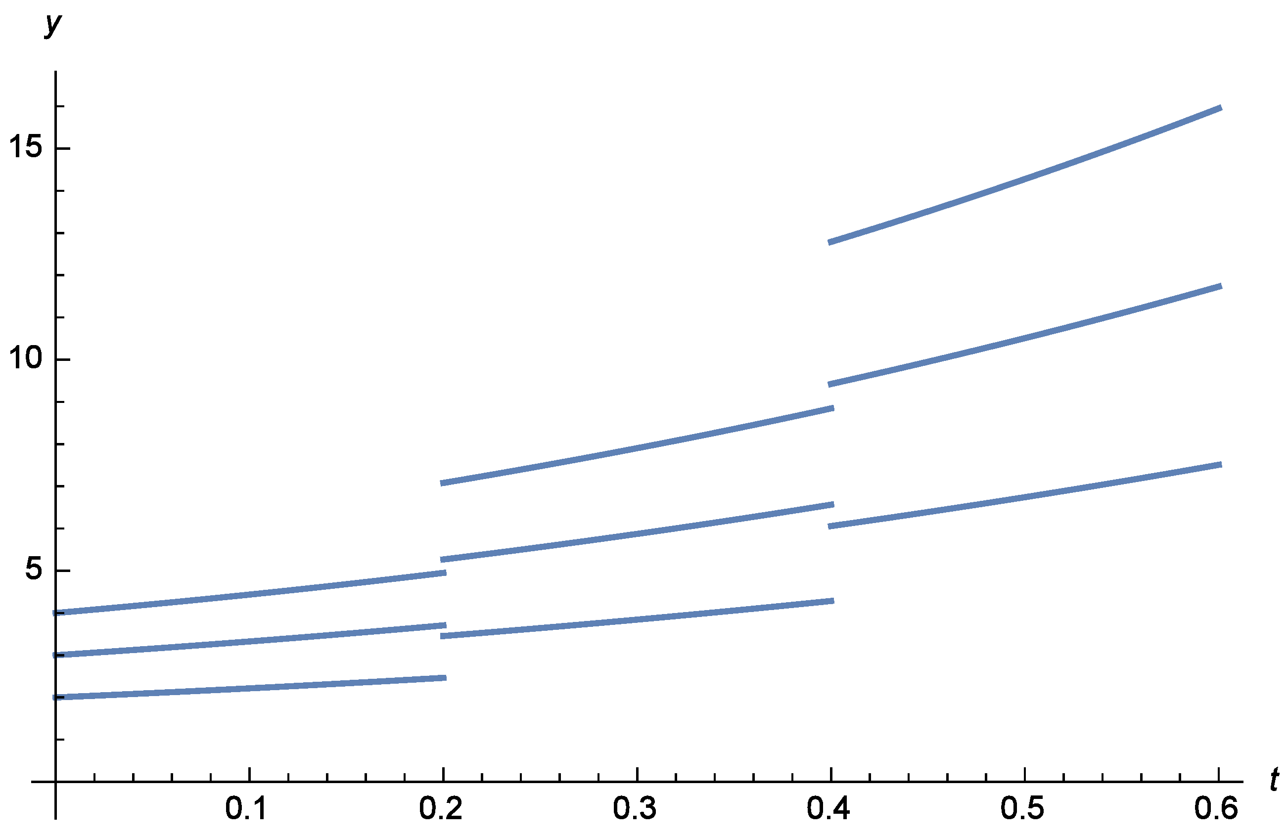
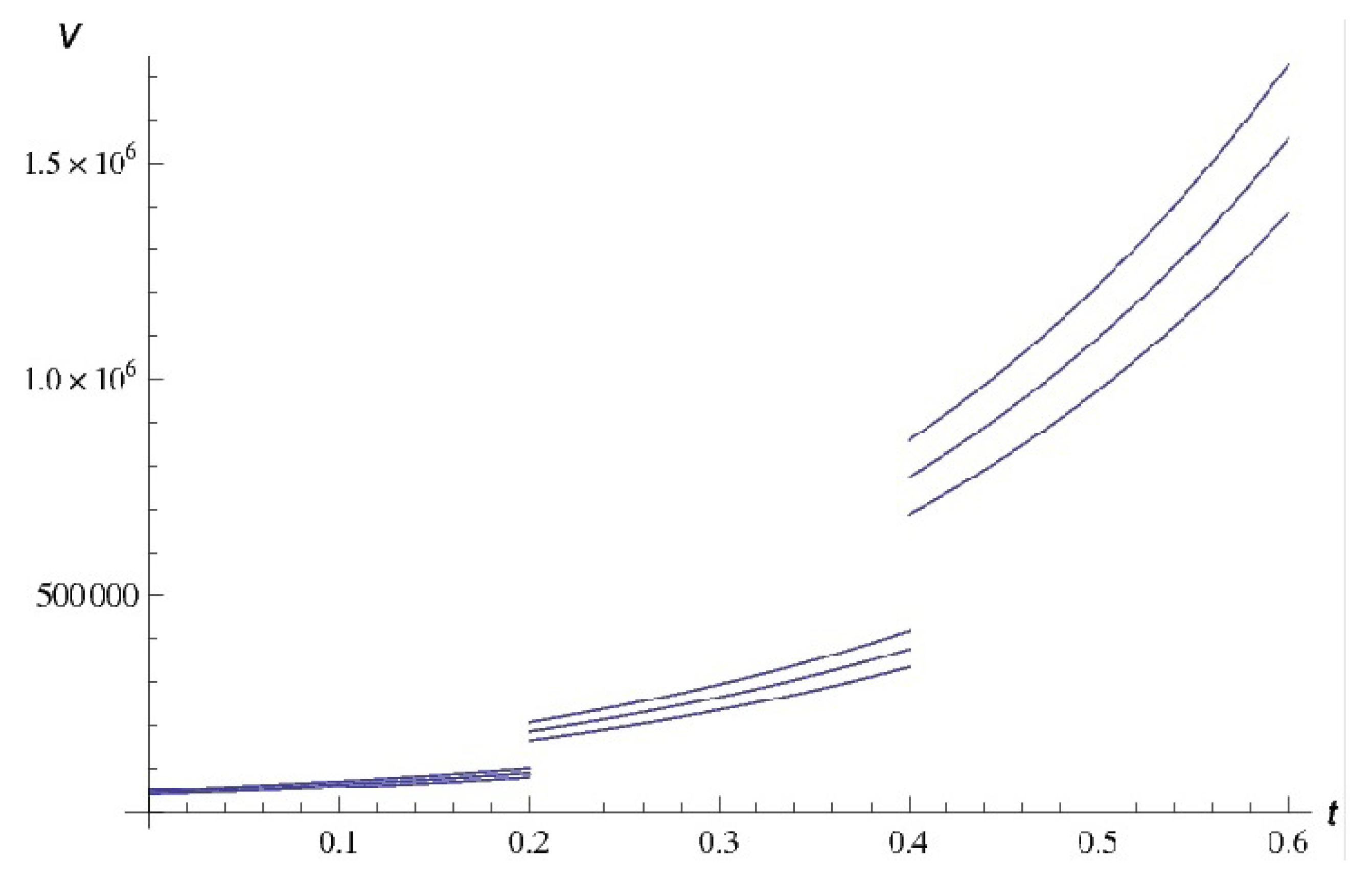
  • Case II. Periodic Compounding: Let us assume that an amount of money P is deposited in a bank account to receive interest at a constant rate I . Here, in contrast to the case of simple interest, we assume that the interest earned will be added to the initial principal periodically. Consequently, the interest will be received not only by the principal, but also by all the interest earned so far. This motivates the following fuzzy difference equation [4]
    V n + 1 = V n ( 1 + I ) , V 0 = P , n = 0 , 1 ,
    The authors of Reference [4] have studied the compound interest problem considering a new factor e n , which is added into the equation, denoting the deposits realized during the life of the account
    V n + 1 = V n ( 1 + I ) + e n , V 0 = P , n = 0 , 1 ,
    It is natural to use fuzzy number for the extra deposits because we do not know certainly the number of deposits that the customer will make during the period of investment.
  • Case III. Continuous Compounding: In this case, the rate of growth of the deposit is proportional to the current wealth. In the periodic compounding, if we consider limit case as n , we get V ( t ) = e t I P , which is the solution of the following Cauchy problem [24]
    V ( t ) = I V ( t ) , V ( 0 ) = P .
    This is known as the continuous compounding, where the corresponding growth factor is e t I .
Remark 3
([24]). For the fixed principal P and interest rate I, the continuous compounding produces the higher future value than periodic compounding with any frequency n .
Example 2.
In the following, by using the results of Section 4, we introduce a new mixed continuous-discrete fuzzy model to study the future value of money. Consider the following fuzzy differential-difference equation
V n ( t ; F n ) = I V n ( t ; F n ) , t ( t n , t n + 1 ] , V n ( t n + ; F n ) = F n , n = 0 , 1 ,
F n + 1 = V n ( t n + 1 ; F n ) + e n , n = 0 , 1 ,
where the initial value F 0 = P . Let us consider triangular fuzzy numbers F 0 = ϕ , ( ϕ + ρ ) 2 , ρ and e n = a n s , s + t 2 , t , where their membership functions are given by
F 0 ( x ) = 2 x + 2 ϕ ϕ ρ , x [ ϕ , ( ϕ + ρ ) 2 ) , 2 x + 2 ρ ρ ϕ , x [ ( ϕ + ρ ) 2 , ρ ) , 0 , o t h e r w i s e ,
and
e n ( x ) = 2 x + 2 a n s a n ( s t ) , x [ a n s , a n ( s + t ) 2 ) , 2 x + 2 a n t a n ( t s ) , x [ a n ( s + t ) 2 , a n t ) , 0 , o t h e r w i s e .
Hence, their level sets are given by
F 0 α = α ( ρ ϕ ) + 2 ρ 2 , α ( ϕ ρ ) + 2 ϕ 2 , e n α = a n 2 α ( t s ) + 2 s , α ( s t ) + 2 t ,
for all α [ 0 , 1 ] . Then, according to the Formula (13), we obtain the solution of the fuzzy differential-difference Equations (23) and (24) is
V n ( t ; F n ) = F 0 e I ( t t 0 ) + i = 0 n 1 e i e I ( t t i + 1 ) .
In particular, we consider I = 3.5 , t n = 0.2 n , n = 0 , 1 , and F 0 , e n are fuzzy numbers whose level sets are given by
F 0 α = 50000 + 5000 [ 1 + α , 1 α ] , e n α = 200 ( n + 1 ) [ 9 + α , 11 α ] .
Finally, the solution of fuzzy differential-difference Equations (23) and (24) is determined by the Formula (25) and its graphical representation with α = 0 , 1 is shown in Figure 2.
Here, the initial value of the deposit is the triangular fuzzy number ( 45 , 000 , 50 , 000 , 55 , 000 ) . Using the FDE (23), we obtain the solution on ( 0 , 0.2 ] . At t = 0.2 , we have an impulsive jump such that we can obtain the value at t 1 + by (24). To obtain the solution on ( 0.2 , 0.4 ] , we use the FDE (23) with initial value F 1 . By following this procedure, we obtain the solution on [ 0 , 0.6 ] in Figure 2.

6. Conclusions

In the present paper, a fuzzy differential-difference equation is proposed to model the mixed continuous-discrete phenomena. We presented the dynamical process in the intervals by a fuzzy differential equation and impulsive jumps in some points by the corresponding fuzzy difference equation. This study generalizes the results of Reference [15] to the fuzzy set theory to consider the uncertain factors in differential equations and difference equations. By this approach, we modeled the uncertainty in initial values and parameters of the differential-difference equations. The general solution of linear fuzzy differential-difference equations is presented, too. Finally, the applicability of the model is illustrated by studying the time value of money in finance.
For further research, we propose to extend these results to study the existence of both (i)-differentiable and (ii)-differentiable solutions of the mixed continuous-discrete fuzzy model corresponding to each case of a. The current work opens up many potential results in studying control problems or numerical algorithms for the fuzzy differential-difference equations, that are inspired by pioneer works [25,26,27,28,29].

Author Contributions

All authors contributed equally. All authors have read and agreed to the published version of the manuscript.

Funding

This project was supported by Researchers Supporting Project number (RSP-2020/210), King Saud University, Riyadh, Saudi Arabia.

Conflicts of Interest

The authors declare no conflict of interest. The writers state that they have no known personal relationships or competing financial interests that could have appeared to affect the work reported in this work.

References

  1. Chakraverty, S.; Tapaswini, S.; Behera, D. Fuzzy Differential Equations and Applications for Engineers and Scientists; Taylor& Francis: Oxfordshire, UK, 2016. [Google Scholar]
  2. Bede, B. Mathematics of Fuzzy Sets and Fuzzy Logic; Springer: London, UK, 2013. [Google Scholar]
  3. Chalco-Cano, Y.; Román-Flores, H. On new solutions of fuzzy differential equations. Chaos Solitons Fractals 2008, 38, 112–119. [Google Scholar] [CrossRef]
  4. Chrysafis, K.A.; Papadopoulos, B.K.; Papaschinopoulos, G. Papaschinopoulos, On the fuzzy difference equations of finance. Fuzzy Sets Syst. 2008, 159, 3259–3270. [Google Scholar] [CrossRef]
  5. Khastan, A. New solutions for first order linear fuzzy difference equations. J. Comput. Appl. Math. 2017, 312, 156–166. [Google Scholar] [CrossRef]
  6. Papaschinopoulos, G.; Papadopoulos, B.K. On the fuzzy difference equation xn+1 = A + x n x n m . Fuzzy Sets Syst. 2002, 129, 73–81. [Google Scholar] [CrossRef]
  7. Villamizar-Roa, E.J.; Angulo-Castillo, V.; Chalco-Cano, Y. Existence of solutions to fuzzy differential equations with generalized Hukuhara derivative via contractive-like mapping principles. Fuzzy Sets Systems 2015, 265, 24–38. [Google Scholar] [CrossRef]
  8. Bede, B.; Rudas, I.J.; Bencsik, A.L. First order linear fuzzy differential equations under generalized differentiability. Inform. Sci. 2007, 177, 1648–1662. [Google Scholar] [CrossRef]
  9. Deeba, E.Y.; de Korvin, A. Analysis by fuzzy difference equations of a model of CO2 level in the blood. Appl. Math. Lett. 1999, 12, 33–40. [Google Scholar] [CrossRef] [Green Version]
  10. Kaleva, O. Fuzzy differential equations. Fuzzy Sets Syst. 1987, 24, 301–317. [Google Scholar] [CrossRef]
  11. Papaschinopoulos, G.; Stefanidou, G. Boundedness and asymptotic behaviour of the solutions of a fuzzy difference equation. Fuzzy Sets Syst. 2003, 140, 523–539. [Google Scholar] [CrossRef]
  12. Rodríguez-López, R. On the existence of solutions to periodic boundary value problems for fuzzy linear differential equations. Fuzzy Sets Syst. 2013, 219, 1–26. [Google Scholar] [CrossRef]
  13. Buckley, J.J. The fuzzy mathematics of finance. Fuzzy Sets Syst. 1987, 21, 257–273. [Google Scholar] [CrossRef]
  14. Córdova, J.D.; Molina, E.C.; López, P.N. Fuzzy logic and financial risk. A proposed classification of financial risk to the cooperative sector. Contaduría Adm. 2017, 62, 1687–1703. [Google Scholar] [CrossRef]
  15. Kwapisz, M. On difference equations arising in mathematics of finance. Nonlinear Anal. Theory Methods Appl. 1997, 30, 1207–1218. [Google Scholar] [CrossRef]
  16. Diamond, P.; Kloeden, P. Metric Spaces of Fuzzy Sets; World Scientific: Singapore, 1994. [Google Scholar]
  17. Gasilov, N.; Amrahov, S.E.; Fatullayev, A.G. Solution of linear differential equations with fuzzy boundary values. Fuzzy Sets Syst. 2014, 257, 169–183. [Google Scholar] [CrossRef]
  18. Nieto, J.J.; Rodríguez-López, R.; Franco, D. Linear first order fuzzy differential equations. Int. J. Uncertain. Fuzziness Knowl.-Based Syst. 2006, 14, 687–709. [Google Scholar] [CrossRef]
  19. Nieto, J.J.; Rodríguez-López, R.; Georgiou, D.N. Fuzzy differential systems under generalized metric spaces approach. Dyn. Syst. Appl. 2008, 17, 1–24. [Google Scholar]
  20. Khastan, A.; Rodríguez-López, R. On the solutions to first order linear fuzzy differential equations. Fuzzy Sets Syst. 2016, 295, 114–135. [Google Scholar] [CrossRef]
  21. Papaschinopoulos, G.; Papadopoulos, B.K. On the fuzzy difference equation xn+1 = A + B x n . Soft Comput. 2002, 6, 456–461. [Google Scholar] [CrossRef]
  22. Lakshmikantham, V.; Trigiante, D. Theory of Difference Equations: Numerical Methods and Applications; Academic Press: New York, NY, USA, 1988. [Google Scholar]
  23. Kacprzyk, J.; Fedrizzi, M. Fuzzy Regression Analysis; Physica-Verlag: Heidelberg, Germany, 1992. [Google Scholar]
  24. Capinski, M.; Zastawniak, T. Mathematics for Finance: An Introduction to Financial Engineering; Springer: London, UK, 2003. [Google Scholar]
  25. Dong, N.P.; Long, H.V.; Khastan, A. Optimal control of a fractional order model for granular SEIR epidemic model. Commun. Nonlinear Sci. Numer. Simulat. 2020, 88, 105312. [Google Scholar] [CrossRef]
  26. Mazandarani, M.; Kamyad, A.V. Modified fractional Euler method for solving fuzzy fractional initial value problem. Commun. Nonlinear Sci. Numer. Simul. 2013, 18, 12–21. [Google Scholar] [CrossRef]
  27. Mazandarani, M.; Zhao, Y. Fuzzy Bang-Bang control problem under granular differentiability. J. Franklin Inst. 2018, 355, 4931–4951. [Google Scholar] [CrossRef]
  28. Son, N.T.K.; Dong, N.P.; Son, L.H.; Abdel-Basset, M.; Manogaran, G.; Long, H.V. On the stabilizability for a class of linear time-invariant systems under uncertainty. Circ. Syst. Signal Process. 2020, 39, 919–960. [Google Scholar] [CrossRef]
  29. Son, N.T.K.; Dong, N.P.; Long, H.V.; Son, L.H.; Khastan, A. Linear quadratic regulator problem governed by granular neutrosophic fractional differential equations. ISA Trans. 2019, 97, 296–316. [Google Scholar] [CrossRef] [PubMed]
Figure 1. The solution of the fuzzy differential-difference Equations (21) and (22) for α = 0.1 .
Mathematics 08 01808 g001
Figure 2. The solution of fuzzy differential-difference Equations (23) and (24) on the interval [ 0 , 0.6 ] with α = 0 , 1 .
Mathematics 08 01808 g002
Publisher’s Note: MDPI stays neutral with regard to jurisdictional claims in published maps and institutional affiliations.

