Abstract
This paper addresses a collaborative multi-carrier vehicle routing problem (CMCVRP) where carriers tackle their orders collaboratively to reduce transportation costs. First, a hierarchical heuristics algorithm is proposed to solve the transportation planning problem. This algorithm makes order assignments based on two distance rules and solves the vehicle routing problem with a hybrid genetic algorithm. Second, the profit arising from the coalition is quantified, and an improved Shapley value method is proposed to distribute the profit fairly to individual players. Extensive experiment results showed the effectiveness of the proposed hierarchical heuristics algorithm and confirmed the stability and fairness of the improved Shapley value method.
1. Introduction
With the rapid development of electronic commerce, logistics service providers—i.e., carriers—are under pressure to improve their efficiencies and service qualities to stay competitive in a fierce business environment. For carriers, one of the most common ways to deliver goods is road transportation. According to the statistical pocketbook released by the Directorate-General for Mobility and Transport (DG Move) of the European Commission [1], during 2015 and 2016 road transportation accounted for 49% of the total transportation of freight in the European Union, 33% in China, 39% in the United States, and around 50% in Japan. In the road transportation sector, the growing competition among companies and the increasing expectations of customers for service quality creates the requirement for small logistics companies to manage their distribution business more efficiently. Thus, companies are enforced to collaborate and establish a coalition to optimize their logistics operations. In the coalition, carriers can exchange their complementary orders to reduce transportation costs. In addition to increasing the efficiency of the carriers, this type of partnership also serves ecological goals. According to the European Commission [1], transportation Greenhouse Gas (GHG) emissions accounted for 26.7% of the total emissions, where road transportation emissions accounted for 72% of total transportation emissions. It can be expected that GHG emissions can be reduced through collaboration among logistics companies. In this study, the collaboration refers to horizontal cooperation, which is distinguished from vertical cooperation, in which a company cooperates with its upstream-downstream firms. In horizontal cooperation, organizations on the same level of the supply chain form a coalition to reduce transportation costs and optimize logistics operations.
Figure 1 shows the comparisons between the non-collaborative multi-carrier vehicle routing problem (NCMCVRP) and collaborative multi-carrier vehicle routing problem (CMCVRP). In the CMCVRP, each carrier i exchanges its orders with other carriers to obtain a more rational assignment R’(i) of orders and minimize the cost of the collaboration. In the NCMCVRP, each company intends to minimize its cost Ci depending on its order set Ri.
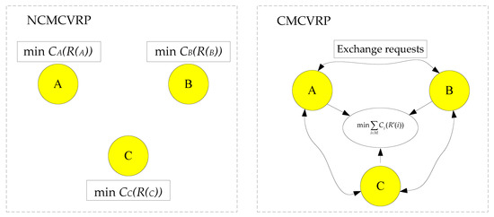
Figure 1.
Comparison between the NCMCVRP and the CMCVRP.
Generally, two tasks are identified as being essential in the CMCVRP. First, the transportation planning of the coalition should be obtained by assigning the total orders. This task is carried out at the coalition level to find more opportunities for collaboration and reduce the total costs. Second, the profit arising from the partnership must be quantified and distributed to each player. A fair profit distribution method is required to ensure the stability of the coalition and promote collaboration. The objective of the CMCVRP is to minimize the total transportation cost of the coalition and then share the gained profit fairly among the players.
The CMCVRP is a variant of a multi-depot vehicle routing problem (MDVRP). Both of these two problems are derived from the classical vehicle routing problem (VRP). The VRP was derived from the traveling salesman problem [2] and was first proposed by Dantzig and Ramser in 1959 [3], which involved the design of a set of minimum-cost vehicle routes, originating and terminating at a central depot, for a fleet of vehicles that services a set of customers with known demands [4]. Since 1959, the VRP has been studied extensively, and many different approaches have been proposed and developed. These approaches include a two-stage method [5], genetic algorithms (GA) [6], a probability matrix-based particle swarm optimization (PSO) [7], a simulated annealing (SA) algorithm [8], ant colony optimization (ACO)-based techniques [9], and a fast Tabu search (TS) algorithm [10]. All the methods mentioned above can well address VRP, but they have different characteristics. The previous two-stage method allocated customers to vehicles first and solved several small TSPs second using a maximum neuron model. The results showed that this method was effective in terms of the quality of solutions and the computational time [5]. The GA-based method in [6] also belonged to a two-stage method, which used GA to determine the groups of customers served by vehicles and the Nearest Neighborhood heuristic (NN) to build the route of each vehicle. The results indicated that the proposed method could achieve good solutions for CVRP instances with a low computational cost. In [7], PSO was proposed to address CVRP using a probability matrix for particle encoding and decoding. The results based on benchmark instances of CVRP have confirmed its effectiveness. Similarly to GA and PSO, ACO is a metaheuristic algorithm which simulates the decision-making processes of ant colonies as they forage for food. In [9], the method for addressing CVRP using ACO could find solutions within 1% of known optimal solutions. Different from the GA, PSO, and ACO methods, the SA and TS algorithms belong to the local search method that searches for solution space beginning with an initial individual. Combining traditional SA or TS methods with neighborhood search techniques, the computational effectiveness and efficiency of SA or TS to solve VRP can be significantly improved [8,10]. Recently, some new methods have been proposed to deal with VRP more efficiently by combining two or more types of algorithms. Zhang et al. [11] developed an interesting approach called the evolutionary scatter search particle swarm optimization algorithm (ESS-PSO) for the VRP with time windows (VRPTW). In ESS-PSO, the PSO and ESS algorithms worked in a cascade learning architecture. Experiments with the Solomon benchmark verified that ESS-PSO can achieve very competitive results. Wu et al. [12] proposed an ant colony optimization algorithm based on improved brainstorm optimization (IBSO-ACO) to solve the VRP with soft time windows. In IBSO-ACO, an improved brainstorm optimization algorithm was used to enrich the diversity of the population obtained by ACO. Extensive experiment results have confirmed that their methods could achieve better solutions than the traditional ant colony algorithm and converge more quickly. For a detailed survey of the methods used to solve VRP, readers are referred to [13].
Studies in the field of MDVRP are rather limited compared to the classical VRP due to the complexity of its distribution network. Ezugwu et al. [14] adopted an enhanced intelligent water drops algorithm for the MDVRP. This algorithm incorporated a simulated annealing algorithm as a local search method to avoid being trapped into local minima. De Oliveira [15] proposed a co-evolutionary algorithm in a parallel environment to solve the MDVRP. The results showed that the proposed method could receive high-quality solutions quickly. For a detailed survey of the methods used to solve the MDVRP, readers are referred to [16].
To solve practical and complicated issues in real life, MDVRP has been extended to more variants with more constraints and objectives. Alinaghian and Shokouhi [17] developed a mathematical model for a multi-depot multi-compartment vehicle routing problem where the cargo space of each vehicle had multiple compartments, and each compartment was dedicated to a single type of product. Jabir et al. [18] designed a hybrid ant colony-variable neighborhood search algorithm for a multi-depot green vehicle routing problem that focused on incorporating the environmental impact on route design. To cut the cost of third-party logistics companies, Shen et al. [19] constructed a model called the low-carbon multi-depot open vehicle routing problem, with time windows to minimize the total costs.
As a new variant of MDVRP, the CMCVRP aims at improving the transportation efficiency as well as the service quality by establishing a coalition among several carriers to collaboratively deliver goods to customers. Liu et al. [20] proposed a two-phase heuristic algorithm for a full truckloads multi-depot capacitated vehicle routing problem. The objective was to minimize empty vehicle movements. Perez-Bernabeu et al. [21] focused on horizontal cooperation in road transportation and addressed it as an MDVRP using an iterated local search algorithm. Montoya-Torres et al. [22] proposed collaborative strategies for goods delivery in city logistics, where several companies united to reduce the transportation distance. These studies did enrich the research on the CMCVRP, but the profit sharing among the players was neglected.
Profit sharing (also called cost allocation) is essential to ensure the stability of a coalition. Cruijsse et al. [23] discussed the potential advantages and disadvantages of cooperation in logistics and indicated that a fair profit sharing mechanism is one of the most prominent advantages of the collaborations. That is to say, carriers would not be willing to join a coalition if the profit sharing method was not fair. The previous studies on profit sharing methods can be categorized into four types: proportional, Shapley value, nucleolus, and equal profit methods. A proportional cost allocation method was proposed by Ozener [24] to solve an inventory routing problem, and the experimental results showed that it performed better than traditional proportional allocation schemes. Defryn et al. [25] employed the volume-based allocation rule—i.e., the proportional method—to solve the cost allocation problem in a cooperative clustered vehicle routing problem. Kimms and Kozeletskyi [26] proposed a Shapley value-based cost allocation in the cooperative traveling salesman problem and applied it as the allocation rule in cooperation for planning decisions. Additionally, as a cost allocation method, the Shapley value was integrated into the optimization of order bundling in a cooperative multi-shipper problem [27]. GotheLundgren et al. [28] employed a nucleolus method to address the vehicle routing cost allocation problem, trying to minimize the maximum discontent among the players in a cooperative game. Frisk et al. [29] developed a novel profit sharing mechanism called an equal profit method to distribute the benefits as similarly as possible for all the participants in solving a collaborative transportation planning problem in a wood flow chain in the forestry industry.
The four types of profit sharing methods mentioned above are disparate from each other due to their specific allocation mechanisms. For example, the Shapley value is for allocating the profit based on the margin contributions in all possible coalitions, while the proportional method is for distributing the profit based on the volume or the amount of the goods. The nucleolus method minimizes maximum discontent among the players in a co-operative game, and the equal profit method aims to minimize the difference of relative profits among participants. Additionally, even for the same allocation mechanism, the allocation methods are different according to the specific problems. Thus, the CMCVRP requires a specific profit sharing or cost allocation method based on an allocation mechanism.
In summary, considerable research has been conducted in the field of CMCVRP. However, to the best of our knowledge, studies on the CMCVRP, including both transportation planning and profit sharing, are rare. On the one hand, the transportation planning of the coalition is supposed to be obtained by assigning the total orders. On the other hand, a fair allocation method is required to distribute the profit arising from the coalition to maintain the stability of the collaboration.
This paper aims at addressing transportation planning and profit sharing issues in the CMCVRP. First, a hierarchical heuristics algorithm is proposed to solve the transportation planning problem using two steps: (1) make order assignments based on two distance rules, and (2) solve the vehicle routing problem with a hybrid genetic algorithm. Second, the profit obtained from the collaboration is quantified and allocated to individual players using an improved Shapley value method. Tests based on benchmark instances have confirmed the effectiveness of the proposed hierarchical heuristics algorithm. Additionally, the stability and fairness of the proposed profit sharing method have been verified by solving 10 generated instances. Compared to the existing studies, we try to make a contribution by (1) proposing the methodology for carriers in the field of electronic commerce to conduct horizontal collaboration, (2) focusing on the collaborative multi-carrier vehicle routing problem (CMCVRP) and formulating an optimization model for the transportation planning process and the game model for profit sharing, and (3) designing methods for addressing transportation planning and profit sharing issues in the CMCVRP.
The remainder of the paper is organized as follows. Section 2 describes the collaborative multi-carrier vehicle routing problem. Section 3 introduces the proposed method for transportation planning and profit sharing tasks. Section 4 presents the numerical experiments and analyses of the results. Finally, Section 5 summarizes the main conclusions of this paper and discusses some future work.
2. Problem Description
In this study, transportation planning and profit sharing tasks are solved independently. The transportation planning problem is first solved to obtain a solution with minimum travel costs, and then the profit is quantified and fairly allocated to individual players. Thus, two models are required for these two stages. In the stage of transportation planning, the problem can be modeled as a special MDVRP. In the stage of profit sharing, the problem is constructed as a game model.
To reduce transportation costs, carriers collaborate by assigning their orders and rearrange their transportation plans. Figure 2 depicts an example of the CMCVRP, where the number of carriers is three.
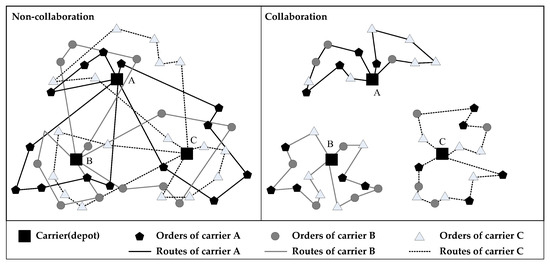
Figure 2.
An example of the CMCVRP with three carriers.
2.1. The Model of Transportation Planning
The objective of transportation planning is to obtain an optimum scheme with minimum logistics costs of the coalition. There are the following assumptions in this stage:
- (1)
- Each route starts and ends at the same carrier depot;
- (2)
- Each order is serviced exactly once by a vehicle;
- (3)
- The total demands of each route should not exceed the vehicle’s capacity;
- (4)
- The goods among different carriers are homogeneous.
Assume that there are m carriers in a coalition. Carriers use identical vehicles with a fixed capacity and share their vehicles to deliver goods. The number of vehicles is sufficient. For the formulation of the mathematical model, the following parameters are introduced:
- M: set of carriers;
- m: number of carriers;
- C: capacity of vehicles;
- V: set of nodes, including all carriers and orders;
- O: set of orders;
- n: number of orders;
- K: set of vehicles;
- v: number of vehicles;
- dij: distance between node i and node j, ;
- qi: demand for order i, , qi > 0;
- xijk: if vehicle k travels from node i to node j, xijk = 1, otherwise, xijk = 0, , .
The objective is to minimize the total travel distance of all the vehicles within the coalition. The model of transportation planning is as follows:
Objective:
Subject to:
In this model, constraints (2) and (3) guarantee that each request is satisfied by one and only one vehicle. Constraint (4) represents the route continuity. Constraint (5) describes the vehicle capacity condition. Constraints (6) and (7) verify the vehicle availability. Constraint (8) provides sub tour elimination. Finally, the formula (9) defines the values of decision variable xijk.
2.2. The Model of Profit Sharing
When the scheme of the coalition with minimum cost is obtained in the stage of transportation planning, the profit gained in the collaboration will be quantified and allocated to individual players.
Let Ci be the cost of carrier i in non-collaborative case, and be the total costs of carriers in coalition M. The minimum travel cost of coalition M in a collaborative case is denoted as C(M). Assume the profit generated in the collaboration is v(M), then it is equal to . The profits of carriers are equal to 0 in the non-collaborative case.
The objective of profit sharing is to allocate the benefits fairly to players based on a specific mechanism Fm, as shown in Equation (10), where denotes the profit allocated to carrier i.
The model of profit sharing is as follows:
Objective:
Subject to:
Constraint (11) represents that the profit is fully allocated to players. Constraint (12) verifies the stability of the allocation mechanism in the sense that there is no sub-coalition S (), such that its players would get better outcomes by deviating from the grand coalition M. Constraint (13) shows that the profits allocated to carriers should not be less than the profits when they act alone.
3. The Proposed Method
3.1. Transportation Planning Based on HHA
A hierarchical heuristic algorithm (HHA) is proposed to address transportation planning, where the first step is to assign total orders by exchanging customer orders among participants based on two distance rules described below. After that, the orders of each carrier are fixed, and a hybrid genetic algorithm (HGA) is proposed to address the vehicle routing problem of individual carriers.
3.1.1. Order Assignment
The assignment employs two distance rules: (1) the closest carrier and (2) the closest neighborhood. Firstly, the term fuzzy node is defined as the node which cannot be assigned to its closest carrier and F is the set of fuzzy nodes. Concerning the two distance rules and fuzzy nodes, the assignment process is divided into two phases, where the first phase is to deal with the nodes that can be allocated to their closest carriers, and these nodes are defined as non-fuzzy nodes. The set of non-fuzzy nodes is defined as NF. The second phase is to allocate fuzzy nodes to the carriers which contain their closest neighborhoods. Here the closest neighborhood of a fuzzy node refers to the non-fuzzy node that is closest to the fuzzy node.
For an order j, define , where and denote the distance between order j and the depots in carrier x, y, respectively. Assume that the number of carriers is m and each carrier has its serial number. Define the distance coefficient , which reflects the difficult degree of an order being allocated to its nearest carrier. The greater the difference between and 1, the more fuzzy nodes generated after the first assignment. The allocation criterion is as follows:
- If , order j will be distributed to carrier 1, where ;
- If and , order j will be distributed to carrier y where , , ;
- If , order j will be distributed to carrier m, where .
The node that cannot be assigned to a specific carrier based on the allocation criterion mentioned above will be appended to the fuzzy node set F. Then, these nodes are assigned to the carrier containing their closest neighborhood. During this process, the distance coefficient is a key parameter that determines the numbers of fuzzy nodes. The smaller the value of , the more fuzzy nodes. The more fuzzy nodes are, the more orders are not assigned to their nearest carrier. When all the order nodes are fuzzy nodes, the result of the order assignment is similar to that of random allocation. Therefore, the appropriate value of should be determined to generate the appropriate number of fuzzy nodes. Preliminary tests showed that when is equal to 0.8, the results of the order assignment can generate better solutions with less cost. In this situation, most of the orders are distributed to their nearest carrier and a small part to the carrier containing their nearest neighborhood.
3.1.2. Solving the Vehicle Routing Problem with HGA
This paper develops a hybrid genetic algorithm (HGA) to deal with the vehicle routing problem in the stage of transportation planning. The HGA integrates the local search technique and greedy algorithm into the crossover operator to generate feasible solutions. Figure 3 depicts the data processing in HGA, where N denotes the population size. HGA starts with generating the initial population. After that, a selection operation is conducted to generate the parent population, and crossover, as well as mutation processes, aim to generate the offspring population. The processes of selection, crossover, and mutation repeat until the ending criterion is reached. Finally, HGA returns the best individual in the above optimization process.
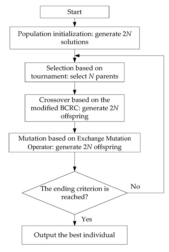
Figure 3.
The flow chart of HGA.
- 1.
- Problem Representation
Most previous studies employed an array filled with index numbers of orders to represent a solution. Unfortunately, this kind of representation can easily produce infeasible solutions in the following recombination process. To overcome this weakness, this study employs a representation that can distinguish sub-routes in a solution by delimiters (see Figure 4). Thus, the recombination is based on the route instead of a single node to avoid the generation of infeasible solutions.
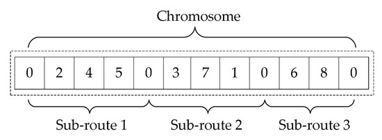
Figure 4.
The representation of the problem.
- 2.
- Population Initialization of HGA
This study adopts the initial strategy composed of a sweep algorithm [30] and a random process. Part of the initial individuals is generated by a sweep algorithm, and others are generated by a random process. The former aims at producing constructed solutions to accelerate convergence, and the latter can ensure the diversity of the population. In our experiments, we found that excessive constructed solutions can decrease population diversity and lead to premature convergence, while excessive random solutions will not influence the quality of solutions but affect the convergence speed. To guarantee population diversity and accelerate the convergence process, the random solutions in the population should account for the majority. In this study, preliminary tests indicated that HGA performs well when the ratio of random solution to constructed solution is 9:1.
Note that all the initial solutions are feasible solutions, indicating that solutions that violate the constraints will be discarded.
- 3.
- Selection Operator of HGA
This study employs the tournament as the selection operator, where several individuals are chosen randomly to compete and the individual with the best fitness value will be selected. This study investigated two types of specific selection strategies: the plus strategy and comma strategy, which can be represented as and , respectively. In these two strategies, denotes the number of parents and represents the amount of offspring. Generally, is larger than . The plus strategy generates from parents new individuals, while the comma strategy generates new parents only from individuals. Preliminary tests have verified that the plus strategy can easily converge to quasi-optimal solutions, while the comma strategy always gives better solutions. Thus, this paper employs the tournament with a comma strategy as the selection operator.
Since infeasible solutions are not allowed to be generated in the evolution process of HGA, potential solutions can be assessed using the objective function (1). Therefore, in the selection process, several individuals are chosen randomly to compete, and the individual with the lowest cost will be selected into the next generation.
- 4.
- Crossover Operator of HGA
Crossover operators for GA can be divided into two groups: (1) crossover based on nodes, and (2) crossover based on routes. The first group includes a classical 1-point crossover (1PX), 2-point crossover (2PX) [31], ordered crossover (OX) [32], linear ordered crossover (LOX) [32], and partial mapping crossover (PMX) [31]. These operators are applied widely in the traveling salesman problem (TSP). Crossover based on routes means that routes in two parents are chosen rather than nodes to carry out the recombination process and generate offspring. This group contains the optimized crossover [33], route copy crossover operator [34], and best cost-best route crossover (BCBRC) [35]. Unfortunately, the above-mentioned crossover operators are not suitable to deal with the VRP directly due to the randomness of the recombination. This randomness can destruct the structure of the sub-route and generate infeasible solutions. Repair algorithms can be applied to deal with infeasible solutions, but they increase the complexity of the GA.
This study proposes a problem-specific crossover operator to obtain the transportation planning of the coalition in the CMCVRP by modifying a well-known crossover operator called Best Cost Route Crossover (BCRC) proposed by Ombuki et al. [36]. The crossover operator integrates the neighborhood search algorithm and the greedy algorithm, aiming at finding the best offspring with maximum fitness while checking the vehicle’s capacity in each sub-route to generate feasible solutions.
The crossover operator carries out the recombination process based on the route to be accordant with the problem representation mentioned above. It consists of two steps: removal and insertion (see Figure 5). The removal step starts with randomly choosing two parents, P1 and P2. Then, a sub-route in P1 and P2 is picked respectively and randomly. The last action of the removal step is to remove the order nodes in the chosen sub-route from the opposite parent. The insertion step is to insert the missing nodes in the offspring. The insertion rules are as follows:
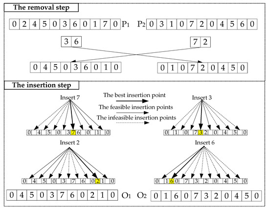
Figure 5.
HGA crossover process.
- (1)
- Insert order j in the alternative positions in the sequence. The alternative positions refer to the intervals between any adjacent orders in each sub-route. During the insertion process, the capacity constraint must be satisfied to generate feasible offspring;
- (2)
- Calculate costs based on Equation (1) after each insertion and find the best insertion point of order j with the best fitness.
- (3)
- A new sub-route can be constructed if all the points violate the capacity constraint.
Let R1 and R2 denote the selected sub-routes in P1 and P2 in the removal step. Assume that the number of order nodes in R1 and R2 is equal to , and the number of orders and sub-routes in one solution is and . Thus, using the representation proposed in this study (see Figure 4), the number of nodes in the initial chromosomes P1 and P2 is including the orders and delimiters between sub-routes. It can be calculated that the maximum computation in the removal step is in 2O() time. In the insertion step, the vehicle’s capacity is first verified for each sub-route before inserting an order j from R1 and R2 into the corresponding parent. Next, each order j is inserted in each alternative position, and the cost based on Equation (1) for each insertion is calculated. After that, order j is deleted in the current alternative position. It can be seen that at each alternative position, three operations are included: insertion, the calculation of cost, and deletion. For the computation simplification, we assume that the number of alternative insertion positions for each order is . Therefore, the maximum computation in the insertion step is in 2O() time. Since and are smaller than , the time complexity of the proposed crossover operator can be simplified as O(). Although the time complexity of the crossover operator used in this study is not high, it is higher than that of the classical 1-point crossover (1PX), 2-point crossover (2PX), ordered crossover (OX), linear ordered crossover (LOX), and partial mapping crossover (PMX). This is because the proposed crossover operator tests all possible insertion positions for each order deleted in the removal step. In our preliminary tests, it was found that the exhaustive tests could bring enough solution quality to motivate such a computational cost, since the solutions returned by the algorithm using the proposed crossover operator were significantly better than those using other crossover operators.
The effectiveness of the crossover operator lies in the insertion step, which incorporates a greedy algorithm and a neighborhood search method. During the insertion process, each available insertion point between any adjacent orders is considered, and the insertion point with the best fitness is selected. Thus, the crossover operator will always find high-quality offspring in the generation. Additionally, the insertion process is subjected to the constraint of the vehicle’s capacity. Thus, infeasible individuals will be avoided.
- 5.
- Mutation Operator of HGA
As we all know, the mutation is a strategy to ensure the diversity of the population by changing several genes of the individuals. Unlike the recombination procedure, the mutation is carried out based on one individual instead of two, which makes it easier than the recombination. This study employs Exchange Mutation Operator as a mutation approach, where two genes are randomly exchanged in one sub-route. As shown in Figure 6, nodes 4 and 1 in the first sub-route are exchanged during the mutation procedure.
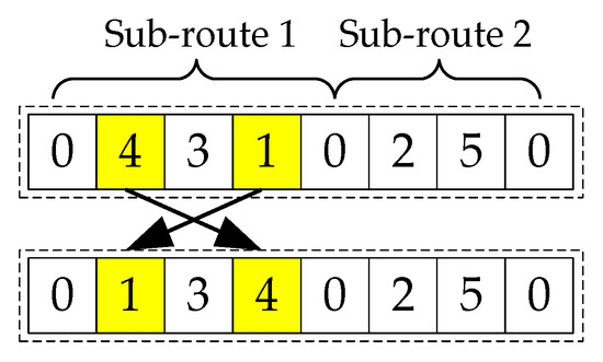
Figure 6.
An example of the Exchange Mutation operator.
- 6.
- Ending Criterion of HGA
This study adopts the ending criterion based on the maximum iterative generations. The preliminary parameter tuning tests showed that generations ranging from 100 to 200 performed well.
3.2. Profit Sharing Based on Improved Shapley Value Method
Since the transportation planning of the coalition has been obtained based on the proposed HHA, the profit arising from the collaboration can then be calculated by comparing the costs between collaborative and non-collaborative cases. The next step is to allocate the gained benefits to individual carriers. Profit sharing is modeled as a game problem aiming at finding a stable and fair allocation scheme for all players. This study proposes a problem-specific profit sharing method for the CMCVRP using an improved Shapley value method [37]. This method assigns a unique distribution (among the players) of a total surplus generated by the coalition of all players. The Shapley value method belongs to the category of cooperative game theory (CGT), where the basic concepts are given below.
3.2.1. Basic Concepts in CGT
Let M = (1,…,m) be the set of all the participants in a coalition, and N be the set of all subsets of M. Define characteristic function v(S): N→, which assigns to each coalition S () a profit value. The characteristic function must satisfy the following two conditions:
The first constraint means that a void coalition has a zero value and the second one, called super additivity, suggests that when two coalitions W and Z collaborate, the profit gained in the collaboration is supposed to be at least the same as when they act alone—i.e., the sum of and .
Define an imputation vector x = (x1,…,xm), referring to the vector of the participants’ profits. It satisfies the rationality and the efficiency, which can be described as below:
Equation (16) presents the individual rationality, meaning that the profit assigned to a player i must be greater than or at least equal to what it could obtain by acting alone—i.e., . The efficiency property of the allocation mechanism is presented in Equation (17), indicating that the total gained benefits are supposed to be fully shared by players. Thus, is equal to the sum of all the participants’ profits—i.e., .
The core of the coalition is the set of imputations when the following condition holds:
The allocation in the core indicates the stability, in the sense that there is no subset S such that its players would get better outcomes by deviating from the grand coalition M. Thus, the benefit of subset S should be less than the sum of profit xi allocated to player i () when it participates in the grand coalition M. As stated in [38], verifying the stability of the method for profit sharing is a common way to verify its effectiveness. Thus, the non-emptiness of the improved Shapley value method should be checked. Note that different profit sharing methods may change the benefits allocated to different players, but they will not influence the general conclusions drawn in this paper. This is because the objective of profit sharing is to allocate the benefits fairly to players, and the methods that satisfy the requirements of profit sharing (the stability mentioned above) will achieve this. Thus, the issue of which method is better is not considered in this study.
3.2.2. Method for Profit Sharing
The proposed improved Shapley value method for profit sharing in the CMCVRP consists of four steps, as detailed below:
Define as the cost of player i when acting alone, and C(S) as the transportation cost of the coalition S. Thus, the characteristics function values are as follows:
Equation (19) denotes the gains obtained from coalition S.
Define the margin contribution of participant i when joining into a coalition S:
Calculate the gains assigned to each carrier by summing all its margin contributions in any possible coalition S. This can be described follows:
where s denotes the number of carriers in the coalition when carrier i joins S. One thing that needs to be mentioned is that s also denotes the sequence when carrier i joins the coalition S. Assume that the number of carriers in a grand coalition is 3, and then the value of s can be equal to 1, 2, or 3.
Verify the non-emptiness of the core in the coalition Constraints (11) and (12).
The Shapley value method satisfies an essential property of a cooperative game: uniqueness. The result of the Shapley value method is unique due to the determinate imputation. Hence, the players will have no room to regret the allocated results and begin an endless bargaining process [38].
3.2.3. An Example with Three Carriers
An assumptive example with three carriers is provided to gain a better understanding of the proposed improved Shapley value method. Table 1 lists all the subsets of the grand coalition, including carriers A, B, and C.

Table 1.
An example of three carriers.
For carrier A, the margin contributions joining into subsets {A}, {A, B}, {A, C}, {A, B, C} are equal to 0, 595, 594, and 628, respectively, based on Equation (20). According to the sequence with which carrier A joins the coalition, the subset {A} has two cases, including {A, B, C} and {A, C, B}; the subset {A, B} has one case, {B, A, C}; the subset {A, C} has one case, {C, A, B}; and the subset {A, B, C} has two cases, including {B, C, A} and {C, B, A}. Table 2 shows the margin contribution of each carrier in all possible coalitions. Thus, the profits allocated to carriers A, B, and C can be obtained based on Equation (21) (=407.5, =503, =502.5).
Table 2.
The margin contribution of each carrier.
Take carrier A for example—when s is equal to 3, it indicates that there are three carriers after carrier A joining the coalition S, and carrier A is the third one to join the coalition. In this case, the value of (m−s)!(s−1)! in Equation (21) is equal to 2, which suggests that there are two kinds of sequences when carrier A joins in coalition S, including {B, C, A} and {C, B, A}, and the margin contributions are equal to 628 in these two coalitions based on Equation (20).
Similarly, when s is equal to 2, it indicates that there are two carriers after carrier A joining the coalition S, and carrier A is the second one to join the coalition. In this case, the value of (m−s)!(s−1)! is equal to 1, which suggests that there is only one kind of sequence when carrier A joins the coalition S. However, the values of also have two cases, which depends on the carriers in the coalition S. If the carriers in the coalition S are A and B, the value of is equal to 595 based on Equation (20), while the value is 594 if the carriers are A and C.
Finally, when s is equal to 1, it indicates that there is only one carrier after carrier A joining the coalition S, and carrier A is the first one to join the coalition. In this case, the value of (m−s)!(s−1)! is equal to 2, which suggests that there are two kinds of sequences when carrier A joins the coalition S—i.e., {A, B, C} and {A, C, B}. The margin contributions are equal to 0 in both of these two coalitions based on Equation (20).
The profit allocated to carrier A can be obtained based on the sum of all margin contributions divided by 6 (3!). Therefore, it can be concluded that the identification of all the possible coalitions that a carrier may join with disparate sequences is the key to obtain the profit allocated to it.
3.3. Solution Framework for the CMCVRP
Figure 7 depicts a solution framework for the CMCVRP, integrating both transportation planning and profit sharing. It can be seen that a classical VRP should be solved for each carrier in the coalition M to quantify the gained profit. Additionally, all of the subsets in the coalition M must be addressed to distribute the gained profit to individual carriers. For a CMCVRP with three carriers (A, B, C), the transportation planning issue is required to be solved seven times, including coalitions {A}, {B}, and {C} in the non-collaboration case and coalitions {A, B, C}, {A, B}, {A, C}, and {B, C} in the collaboration case.
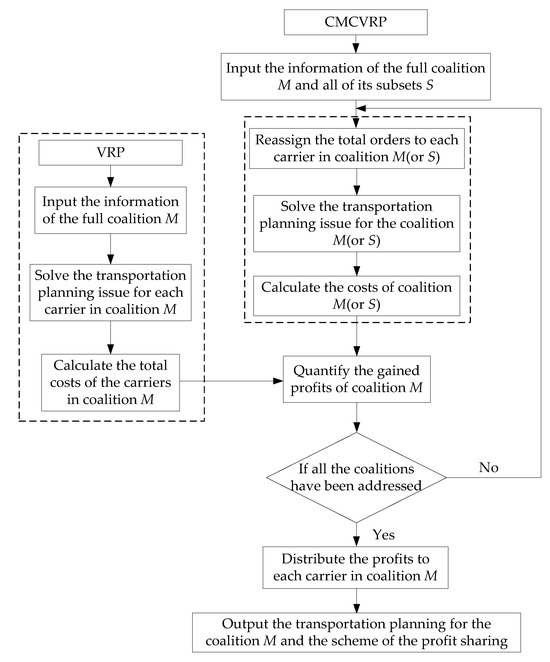
Figure 7.
Solution framework for the CMCVRP.
4. Experimental Results and Discussion
In this section, numerical experiments were conducted to test the performance of the above-mentioned methods for the CMCVRP. Since the CMCVRP was addressed based on two stages in this study—i.e., transportation planning first and profit sharing second (see Section 3)—the experiments were divided into two aspects to test the performance of the proposed methods in these two stages. In Section 4.1, the proposed HHA method for the stage of transportation planning was tested based on MDVRP benchmark instances, since the model in the transportation planning process in CMCVRP is similar to MDVRP (see Section 2.1). After that, 10 cases were generated to test the proposed profit sharing method because CMCVRP has no benchmark instances. These instances were solved by the proposed HHA method to quantify the profit obtained from the collaboration (see Section 4.2). Finally, the profit was allocated to individual partners using the improved Shapley value method, whose effectiveness was confirmed based on the rules in Section 3.2.2 (see Section 4.3).
In the experiments, each instance was solved 30 times, and the best solution with minimum cost (based on Equation (1)) was reported. All the tests were conducted on a Lenovo laptop computer with Windows 10, an Intel i7 processor, and 8 GB of installed RAM.
4.1. Testing the Performance of HHA for Transportation Planning
As mentioned in Section 2, the problem in the stage of transportation planning can be modeled as a special MDVRP. Thus, we tested the performance of HHA based on MDVRP benchmark instances. Table 3 shows the results of HHA in solving MDVRP benchmark instances. The selected seven data sets can be obtained from [39]. Each data set contains the following information: the coordinates of depots and orders, the number of demands for each order, and the capacity of the vehicles. In Table 3, columns n, m, and C show the number of orders, the number of depots, and the capacity of vehicles, respectively. Besides this, BKS denotes the best-known solutions in existing studies. Columns HHAbest and HHAavg show the best and average solutions returned by the HHA method. Gap1 denotes the gap between HHAbest and BKS and equals (HHAbest − BKS)/BKS. Gap2 represents the gap between HHAbest and HHAavg and equals (HHAavg − HHAbest)/HHAbest.
Table 3.
The results of HHA in solving MDVRP benchmark instances.
As shown in Table 3, the maximum gap between the best solutions returned by HHA and BKS is less than 4% (see column Gap1) when solving the seven data sets, so it can be concluded that HHA is effective in addressing MDVRP instances, and then it can be used for solving the transportation planning issues in CMCVRP. Moreover, it can be seen that the gap between the best solutions and the average solutions is small (see column Gap2), indicating the stability of HHA. Since the process of order assignment is deterministic, it can be inferred that the HGA method is stable and can return stable solutions.
In this study, the HGA method is proposed for solving VRP in the process of transportation planning. Additionally, it is used for calculating the transportation cost of each carrier before the collaboration to quantify the gained profit (see Section 3.3). Thus, we also tested the performance of HGA. Table 4 shows the results of HGA when solving VRP benchmark instances selected from [39].
Table 4.
The results of HGA in solving VRP benchmark instances.
As shown in Table 4, the maximum gap between HGAbest and BKS is less than 1% (see column Gap1), indicating the effectiveness of HGA in addressing VRP instances. Additionally, the maximum gap between HGAbest and HGAavg is less than 1% (see column Gap2), which confirms the stability of HGA. Therefore, HHA is used to obtain the solution with the minimum cost for the coalition, and HGA is used to calculate the stand-alone cost of individual carriers. The difference between the cost of the coalition and the total stand-alone cost of all carriers is the profit of the coalition.
4.2. Quantifying the Gained Profit
The profit gained in the collaboration depends on the gap between the cost in the collaborative and non-collaborative cases. The cost in the collaborative case can be obtained based on the solutions of the transportation planning problem using the proposed HHA, while the cost in the non-collaborative case is the sum of each player’s cost when acting alone. Without a loss of generality, this paper studied the coalition with three carriers. Ten grand coalitions were generated randomly, where each coalition had three carriers and the number of orders ranged from 60 to 150.
Table 5 presents the results of transportation planning in ten coalitions. In the tests, each instance was solved 30 times and the best-known solution was reported. Thus, the time reported in Table 5 for solving one instance is the average time of 30 runs. The details of each coalition comprise the following: (1) a serial number of the coalition, S; (2) the number of the orders, n; (3) carriers in each coalition, i; (4) the cost of carrier i in the non-collaboration case, C(i); (5) the cost of carriers in the collaboration case, CCC; (6) cost reduction ratio of carrier i, CRRC (refer to Equation (22)); (7) the number of carriers’ orders in the non-collaboration case, NCONC; (8) the number of carriers’ orders in the collaboration case, NCOC; (9) the proportion of carriers’ orders in a coalition, PCO (refer to Equation (23)); (10) the number of carriers’ vehicles in the non-collaboration case, NCVNC; (11) the number of carriers’ vehicles in the collaboration case, NCVC; (12) the reduction in vehicles, RV; (13) the total non-collaboration costs for coalition S, ; (14) the collaboration costs of coalition S, C(S); (15) the profit gain rate of coalition S, PRCO (refer to Equation (24)).
Table 5.
The results of transportation planning.
At the level of individual players, it can be seen that the cost of each player in each coalition reduces significantly, especially for carrier A, and the cost reduction rates of different carriers are very different (see column CRRC). Note that each carrier is responsible for several orders in the coalition and the proportions are disequilibrium (see columns NCOC and PCO). At the level of the coalition, it is found that the reduction in the total vehicle number is not significant (see column RV), whereas the cost of the coalition decreases markedly with the profit gain rates ranging from 46.5% to 50.3% (see column PRCO).
Table 6 shows the profit gain rates of the coalitions, including both the sub-coalitions ({A, B}, {A, C}, {B, C}) and the grand coalition ({A, B, C}). It indicates that the grand coalition can always obtain the largest profit gain rate in all possible coalitions, which suggests the effectiveness of the collaboration.
Table 6.
The profit gain rates of the coalitions.
4.3. Allocating the Gained Profit
To guarantee the stability of the collaboration, the gained profit must be allocated to the players fairly. The proposed improved Shapley value method distributes the profit based on the margin contributions of the participants, which can ensure the uniqueness of the allocation outcome. However, this outcome may not be stable, which means that the players may not accept the allocation outcome because there is a subset S such that its players will get more profit. Thus, the non-emptiness of the core in the coalition is supposed to be checked.
Table 7 presents the profit allocated to individual carriers based on the improved Shapley value method (see column PRC). Column PRC shows the profit gain rates of the carriers which can be calculated based on Equation (25). Column ARPC presents the average profit gain rates of the carriers in a coalition. To verify the stability of the allocation method, the profits of individual sub-coalitions are calculated to check the non-emptiness of the core in a grand coalition. Table 8 shows the profits gained in sub-coalitions and grand coalitions. It can be seen that the total profit gained in the grand coalition ({A, B, C}) for the carriers is larger than that in any sub-coalition (including {A, B}, {B, C}, {A, C}). Based on constraints (11) and (12), it can be concluded that the core of each coalition is non-empty and the allocation outcome in each grand coalition can satisfy the quality of the stability. Thus, there is no sub-coalition of each grand coalition which has a better outcome for players—i.e., the players can accept the allocation outcomes without bargaining.
Table 7.
The results of profit sharing.
Table 8.
The stability of the allocation method.
The fairness of the proposed method for profit sharing can also be verified based on the principle of “more pay for more work”. The more orders served by a carrier, the more profits they should get. Figure 8 shows the relationship between the profit gain rates of the carriers (PRC, including PRCA, PRCB, and PRCC for carriers A, B, and C, respectively) and the proportions of the carriers’ orders in a coalition (PCO, including PCAO, PCBO, and PCCO for carriers A, B, and C, respectively). PCO can be calculated based on Equation (23). It can be seen that the larger the PCO, the larger the PRC, which confirms the fairness of the proposed improved Shapley value method.
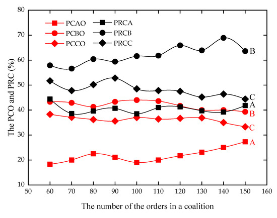
Figure 8.
The relationship between PCO and PRC.
5. Conclusions and Future Work
This paper addressed the collaborative multi-carrier vehicle routing problem (CMCVRP), where several logistics service providers collaborate to reduce transportation costs by exchanging customer orders. The carriers in such a partnership share their information about the vehicles and the orders. The objective is to minimize the total transportation cost of the coalition and then allocate the gained profit fairly to individual players (coalition members).
In this study, we proposed the methodology for carriers in the field of electronic commerce to conduct horizontal collaboration, including both transportation planning and profit sharing. A hierarchical heuristic algorithm (HHA) was proposed to make transportation planning for the coalition. The simulation results have verified the effectiveness of the proposed algorithm in the stage of transportation planning, which indicated that the proposed HHA could provide a solid foundation for the quantification as well as the allocation of the profit in the collaboration. The profit gained from the coalition was quantified and an improved Shapley value method, belonging to the category of cooperative game theory, was provided to allocate the profit based on the margin contributions of the players. The stability of the allocation method has been confirmed by checking the non-emptiness of the core in the coalition.
The results obtained from the tests could provide managers with some implications: (1) horizontal collaboration is worth trying since it can make significant cost savings for the coalition as well as individual partners; (2) the number of players in a coalition can influence the profit gain rates obtained by the players, so the appropriate number of co-operators before forming a coalition should be determined; (3) the selection of a profit sharing method is important because it can influence the stability of the coalition, and the method based on cooperative game theory can well ensure the stability of the cooperation.
This study is the first step towards the full integration of transportation planning and profit sharing in the collaborative multi-carrier vehicle routing problem, where the transportation planning and profit sharing tasks are solved collaboratively to promote the collaboration. However, the method presented in this paper addresses these two tasks independently. This two-staged method cannot ensure the stability of the coalition when using the proportional method for profit sharing. This is due to the fact that the objective of the CMCVRP is to minimize the total cost of the coalition, while the objectives of the individual players are not considered. The transportation planning of the coalition with the minimum cost may not be the best planning for individual players where they may get more profits [25,27]. Thus, the players may not accept the allocation outcome or even quit the coalition. In this study, the proposed improved Shapley value method can ensure the stability of the coalition, since the players could obtain the most profits in the solution in which the coalition obtains the most profits based on the rules in Section 3.2.2. The integrated method for the CMCVRP could be investigated to ensure the stability of the coalition when the proportional method is used for profit sharing. In this integrated method, the objectives at the coalition level and player level were considered simultaneously, making the CMCVRP a multi-objective optimization issue [25,27].
In future work, it will be interesting to develop the integrated method mentioned above for the CMCVRP. Thus, transportation planning and profit sharing stages could be integrated into one model and optimized integrally, considering the benefits of both the coalition and individual carriers. Additionally, more complicated horizontal cooperation optimization issues will emerge with the development of electronic commerce, which can be one potential future research direction. Moreover, considering unexpected random disturbances is interesting and significant for the real-life implementation of horizontal cooperation. Finally, the methodology proposed in this study for horizontal collaboration could be extended to more fields, including emergency logistics, where organizations collaborate to conduct last-mile relief delivery [40].
Author Contributions
Conceptualization, Y.S. and W.S.; Data curation, N.L. and T.Z.; Formal analysis, N.L. and Q.H.; Funding acquisition, Y.S.; Investigation, N.L., Q.H., and T.Z.; Methodology, Y.S. and N.L.; Project administration, Y.S.; Resources, Y.S. and W.S.; Software, N.L. and T.Z.; Supervision, Y.S. and W.S.; Validation, Q.H.; Visualization, N.L.; Writing—original draft, Y.S., N.L., and Q.H.; Writing—review and editing, Y.S., N.L., Q.H., and W.S. All authors have read and agreed to the published version of the manuscript.
Funding
This work was financially supported by the National Key Research and Development Project (no. 2018YFE0197700).
Conflicts of Interest
The authors declare no conflict of interest.
References
- EU Transport in Figures-Statistical Pocketbook. 2018. Available online: https://www.europeansources.info/record/eu-transport-in-figures-statistical-pocketbook-2018/ (accessed on 22 July 2020).
- Hvattum, L.M.; Tirado, G.; Felipe, A. The Double Traveling Salesman Problem with Multiple Stacks and a Choice of Container Types. Mathematics 2020, 8, 979. [Google Scholar] [CrossRef]
- Dantzig, G.B.; Ramser, J.H. The Truck Dispatching Problem. Manag. Sci. 1959, 6, 80–91. [Google Scholar] [CrossRef]
- Sabo, C.; Pop, P.C.; Horvat-Marc, A. On the Selective Vehicle Routing Problem. Mathematics 2020, 8, 771. [Google Scholar] [CrossRef]
- Yoshiike, N.; Takefuji, Y. Solving Vehicle Routing Problems by Maximum Neuron Model. Adv. Eng. Inform. 2002, 16, 99–105. [Google Scholar] [CrossRef]
- De Araujo Lima, S.J.; de Araujo, S.A.; Triguis Schimit, P.H. A Hybrid Approach Based on Genetic Algorithm and Nearest Neighbor Heuristic for Solving the Capacitated Vehicle Routing Problem. Acta Sci. Technol. 2018. [Google Scholar] [CrossRef]
- Kim, B.-I.; Son, S.-J. A Probability Matrix Based Particle Swarm Optimization for the Capacitated Vehicle Routing Problem. J. Intell. Manuf. 2012, 23, 1119–1126. [Google Scholar] [CrossRef]
- Xiao, Y.; Zhao, Q.; Kaku, I.; Mladenovic, N. Variable Neighbourhood Simulated Annealing Algorithm for Capacitated Vehicle Routing Problems. Eng. Optim. 2014, 46, 562–579. [Google Scholar] [CrossRef]
- Bell, J.E.; McMullen, P.R. Ant Colony Optimization Techniques for the Vehicle Routing Problem. Adv. Eng. Inform. 2004, 18, 41–48. [Google Scholar] [CrossRef]
- Chunyu, R. Fast Tabu Search Algorithm for Capacitated Vehicle Routing Problem. Adv. Mater. Res. 2013, 760–762, 1790–1793. [Google Scholar]
- Zhang, J.; Yang, F.; Weng, X. An Evolutionary Scatter Search Particle Swarm Optimization Algorithm for the Vehicle Routing Problem with Time Windows. IEEE Access 2018, 6, 63468–63485. [Google Scholar] [CrossRef]
- Wu, L.; He, Z.; Chen, Y.; Wu, D.; Cui, J. Brainstorming-Based Ant Colony optimization for Vehicle Routine With Soft Time Windows. IEEE Access 2019, 7, 19643–19652. [Google Scholar] [CrossRef]
- Braekers, K.; Ramaekers, K.; Van Nieuwenhuyse, I. The Vehicle Routing Problem: State of the Art Classification and Review. Comput. Ind. Eng. 2016, 99, 300–313. [Google Scholar] [CrossRef]
- Ezugwu, A.E.; Akutsah, F.; Olusanya, M.O.; Adewumi, A.O. Enhanced Intelligent Water Drops Algorithm for Multi-Depot Vehicle Routing Problem. PLoS ONE 2018. [CrossRef] [PubMed]
- De Oliveira, F.B.; Enayatifar, R.; Sadaei, H.J.; Guimaraes, F.G.; Potvin, J.-Y. A Cooperative Coevolutionary Algorithm for the Multi-Depot Vehicle Routing Problem. Expert. Syst. Appl. 2016, 43, 117–130. [Google Scholar] [CrossRef]
- Montoya-Torres, J.R.; Lopez Franco, J.; Nieto Isaza, S.; Felizzola Jimenez, H.; Herazo-Padilla, N. A Literature Review on the Vehicle Routing Problem with Multiple Depots. Comput. Ind. Eng. 2015, 79, 115–129. [Google Scholar] [CrossRef]
- Alinaghian, M.; Shokouhi, N. Multi-Depot Mmulti-Compartment Vehicle Routing Problem, Solved by a Hybrid Adaptive Large Neighborhood Search. Omega 2018, 76, 85–99. [Google Scholar] [CrossRef]
- Jabir, E.; Panicker, V.V.; Sridharan, R. Design and Development of a Hybrid ant Colony-Variable Neighbourhood Search Algorithm for a Multi-Depot Green Vehicle Routing Problem. Transp. Res. Part D 2017, 57, 422–457. [Google Scholar] [CrossRef]
- Shen, L.; Tao, F.; Wang, S. Multi-Depot Open Vehicle Routing Problem with Time Windows Based on Carbon Trading. Int. J. Env. Res. Public Health 2018, 15, 2025. [Google Scholar] [CrossRef]
- Liu, R.; Jiang, Z.; Fung, R.Y.K.; Chen, F.; Liu, X. Two-Phase Heuristic Algorithms for Full Truckloads Multi-Depot Capacitated Vehicle Routing Problem in Carrier Collaboration. Comput. Oper. Res. 2010, 37, 950–959. [Google Scholar] [CrossRef]
- Perez-Bernabeu, E.; Juan, A.A.; Faulin, J.; Barrios, B.B. Horizontal Cooperation in Road Transportation: A Case Illustrating Savings in Distances and Greenhouse Gas Emissions. Intl. Trans. Oper. Res. 2015, 22, 585–606. [Google Scholar] [CrossRef]
- Montoya-Torres, J.R.; Munoz-Villamizar, A.; Vega-Mejia, C.A. On the Impact of Collaborative Strategies for Goods Delivery in City Logistics. Prod. Plan. Control 2016, 27, 443–455. [Google Scholar] [CrossRef]
- Cruijssen, F.; Cools, M.; Dullaert, W. Horizontal Cooperation in Logistics: Opportunities and Impediments. Transp. Res. Part E 2007, 43, 129–142. [Google Scholar] [CrossRef]
- Ozener, O.O.; Ergun, O.; Savelsbergh, M. Allocating Cost of Service to Customers in Inventory Routing. Oper. Res. 2013, 61, 112–125. [Google Scholar] [CrossRef]
- Defryn, C.; Sorensen, K.; Dullaert, W. Integrating Partner Objectives in Horizontal Logistics Optimisation Models. Omega 2019, 82, 1–12. [Google Scholar] [CrossRef]
- Kimms, A.; Kozeletskyi, I. Shapley Value-Based Cost Allocation in the Cooperative Traveling Salesman Problem Under Rolling Horizon Planning. EURO J. Transp. Logist. 2016, 5, 371–392. [Google Scholar] [CrossRef]
- Vanovermeire, C.; Sorensen, K. Integration of the Cost Allocation in the Optimization of Collaborative Bundling. Transp. Res. Part E 2014, 72, 125–143. [Google Scholar] [CrossRef]
- GotheLundgren, M.; Jornsten, K.; Varbrand, P. On the Nucleolus of the Basic Vehicle Routing Game. Math. Program. Ser. B 1996, 72, 83–100. [Google Scholar] [CrossRef]
- Frisk, M.; Gothe-Lundgren, M.; Jornsten, K.; Ronnqvist, M. Cost Allocation in Collaborative Forest Transportation. Eur. J. Oper. Res. 2010, 205, 448–458. [Google Scholar] [CrossRef]
- Gillett, B.E.; Miller, L.R. Heuristic Algorithm for Vehicle-Dispatch Problem. Oper. Res. 1974, 22, 340–349. [Google Scholar] [CrossRef]
- Zhu, K.Q. A Diversity-Controlling Adaptive Genetic Algorithm for the Vehicle Routing Problem with Time Windows. In Proceedings of the 15th IEEE International Conference on Tools with Artificial Intelligence, Sacramento, CA, USA, 5 November 2003; pp. 176–183. [Google Scholar]
- Xing, L.; Rohlfshagen, P.; Chen, Y.; Yao, X. An Evolutionary Approach to the Multidepot Capacitated Arc Routing Problem. IEEE Trans. Evol. Comput. 2010, 14, 356–374. [Google Scholar] [CrossRef]
- Nazif, H.; Lee, L.S. Optimised Crossover Genetic Algorithm for Capacitated Vehicle Routing Problem. Math. Model. 2012, 36, 2110–2117. [Google Scholar] [CrossRef]
- Wang, K.; Lan, S.; Zhao, Y. A Genetic-Algorithm-Based Approach to the Two-Echelon Capacitated Vehicle Routing Problem with Stochastic Demands in Logistics Service. J. Oper. Res. Soc. 2017, 68, 1409–1421. [Google Scholar] [CrossRef]
- Ghannadpour, S.F.; Zarrabi, A. Multi-Objective Heterogeneous Vehicle Routing and Scheduling Problem with Energy Minimizing. Swarm Evol. Comput. 2019, 44, 728–747. [Google Scholar] [CrossRef]
- Ombuki, B.; Ross, B.J.; Hanshar, F. Multi-Objective Genetic Algorithms for Vehicle Routing Problem with Time Windows. Appl. Intell. 2006, 24, 17–30. [Google Scholar] [CrossRef]
- Shapley, L. A Value for N-Person Games. In Contributions to the Theory of Games II; Princeton University Press: Princeton, NJ, USA, 1953; pp. 307–317. [Google Scholar]
- Krajewska, M.A.; Kopfer, H.; Laporte, G.; Ropke, S.; Zaccour, G. Horizontal Cooperation Among Freight Carriers: Request Allocation and Profit Sharing. J. Oper. Res. Soc. 2008, 59, 1483–1491. [Google Scholar] [CrossRef]
- The VRP Web. Available online: http://neo.lcc.uma.es/radi-aeb/WebVRP/ (accessed on 27 July 2020).
- Jiang, Y.P.; Yuan, Y.F. Emergency Logistics in a Large-Scale Disaster Context: Achievements and Challenges. Int. J. Environ. Res. Public Health 2019, 16, 23. [Google Scholar] [CrossRef]
Publisher’s Note: MDPI stays neutral with regard to jurisdictional claims in published maps and institutional affiliations. |
© 2020 by the authors. Licensee MDPI, Basel, Switzerland. This article is an open access article distributed under the terms and conditions of the Creative Commons Attribution (CC BY) license (http://creativecommons.org/licenses/by/4.0/).