Abstract
To follow up on the progress made on exploring the stability investigation of linear commensurate Fractional-order Difference Systems (FoDSs), such topic of its extended version that appears with incommensurate orders is discussed and examined in this work. Some simple applicable conditions for judging the stability of these systems are reported as novel results. These results are formulated by converting the linear incommensurate FoDS into another equivalent system consists of fractional-order difference equations of Volterra convolution-type as well as by using some properties of the Z-transform method. All results of this work are verified numerically by illustrating some examples that deal with the stability of solutions of such systems.
1. Introduction
Undoubtedly, it has been demonstrated, over the past few decades, that the non-integer calculus is a forceful mathematical argument for providing many and more dynamics for lots of ancient as well as modern models. For instance, there are several dynamical models and many real-world applications that were recently handled via this tool such as diffusion modeling [], robot manipulators [], economics [], and many more. As a matter of fact, such branch of calculus, in its two structures (discrete and continuous), requires the order of the functional operator of calculus to be in its fractional-order case for a number of core concepts such as derivatives, integrals, and differences. This indeed allows for creating appropriate mathematical models together with extremely rich and complex dynamics [,]. In the area of the discrete fractional calculus, the explanation of its main concept is referred to in Diaz and Olseronly in 1974 []. After that time, for at least a decade or more, some serious efforts in this field began to appear. Among those efforts, to name a few, is what Miller and Ross proposed in []. They actually established some basic definitions, primary schemes, and properties related to the fundamental theorem []. To date, a lot of researchers are competing in proposing impressive results and methods in regard to this field. Anyhow, for a complete comprehensive description about this branch of calculus, the reader may refer to [,,].
Over the past few years, modeling several chemical and physical phenomena have broadly been carried out using the theory of Fractional-order Difference Systems (FoDSs) []. In fact, the FoDS is employed, with its particular digital data, for the purpose of approximating its corresponding fractional-order differential equations. This allows one to enter them into suitable computer programs and then simulate the obtained results []. However, it was reported in [] that the Z-transform method can solve the linear FoDSs, as it can perform the same matter for the linear Fractional-order Difference Equation (FoDE). The Z-transform method can be, at the same time, employed as a powerful aid tool in discussing the stability analysis of such systems, as declared in [,,,]. However, even so, there are formidable challenges, generally, in proposing a proper tool for performing this task []. Therefore, it might be said that the stability analysis of the FoDSs is not yet developed []. This has motivated, in recent years, many researchers to deal with this dilemma, and as a consequence of this, several other works have preferred it to be the main target of their investigations (see [,,,]). In particular, Abu-Saris and Al-Mdallal developed in [] a theory about the stability of linear FoDSs. However, unfortunately, it was shown that their theorem is difficult to apply. That matter remained until 2015. This year, Čermák et al. developed another simplified and applicable theorem for the same purpose (see []). As far as we know, discussing the stability analysis by providing novel simplified results for Linear FoDS with incommensurate orders remains up until now a recent and mostly unexamined topic. In light of this urgent need, this paper presents some simple applicable conditions for judging the stability of such system by first converting it into another equivalent form that includes FoDEs of the Volterra convolution-type as well as by using the properties of the Z-transform method. All results of this work are provided by examples, so that all plots of the stability of the solutions for systems are exhibited according to given incommensurate orders. However, this paper is organized in the following order. Section 2 introduces some primary preliminaries associated with discrete fractional calculus, while Section 3 discusses some recently established results that have handled the stability of linear commensurate FoDS for the purpose of getting new results in regard to incommensurate orders. Section 4 exhibits several examples to verify all findings, followed by the last section that summarizes the achievements of the whole work.
2. Preliminaries
This section briefly introduces some basic definitions and preliminaries associated with discrete fractional calculus. In all of the definitions below, the function f is defined on , where , for .
Definition 1
([]). The fractional sum operator of a function is expressed as:
where is the order of the operator and .
Definition 2
([]). The fractional Riemann–Liouville difference operator of a function f is defined by:
where is the order of the operator, , and .
Definition 3
([]). The fractional Caputo difference operator of a function f is expressed as:
where is the order of the operator, and .
Lemma 1
([]). Let and . Then,
where is the general binomial coefficient.
Proof.
By Definition 2, one can obtain:
Using Pascal rule yields
□
3. Stability Analysis of the Linear Incommensurate FoDS
In this section, we state some additional results, reported in [,], in order to pave the way for introducing the main results of this work, which will be verified numerically, later on, in Section 4. Such results will clearly show the stability of the linear FoDS with incommensurate orders via some useful conditions formulated as theorems. First of all, consider the following linear incommensurate FoDS:
where is the fractional Caputo difference operator of order , and , for .
The main objective of this work does not explore the separate investigation of the FoDSs, but it especially explores the generalization of some notions and results achieved in the framework of these discrete settings. One of the main features that is reflected from studying such systems is memory. This feature can be revealed by tracking the evolution of any state of these systems, which not only depends on the current solution, but it also depends on the whole history of its development. In general, many literature works seem to agree that these systems possess superior properties as compared to their standard counterpart. It has been shown that the core of their general dynamics solution is heavily dependent on the variations of the fractional-order values. However, most of those literature works are concerned only with studying the dynamic characteristics of linear commensurate FoDSs, which is of course a special case of systems with incommensurate fractional-orders. From the perspective of such orders having different effects on the linear incommensurate FoDSs, several physical phenomena are formulated and accurately described for the purpose of improving the complexity of their solutions over the original systems. For instance, if , then system (5) might be expressed in the commensurate form as follows:
where , , and where . In [], Abu-Saris and Al-Mudalal established some results associated with the stability of the system given in (6) by transforming it into a northern difference system of the Volterra convolution-type as well as using some properties of the Z-transform method. They actually deduced Theorem 1 given below.
Theorem 1
([]). Suppose . The isolated zeroes, of the nonnegative real axis, of
lie inside the unit disk if and only if the zero solution of system (6) is asymptotically stable, where is the identity matrix.
One might notice that, despite their good work, applying such results is, indeed, an extremely difficult task. The justification of that belief is referred to difficulties in determining the zeros of (7). This matter, however, encouraged Čermák et al. to overcome its difficulties. For that purpose, they transformed system (6) into another difference system of Volterra convolution-type and then applied the deduced results of Elaydi et al. in []. In other words, they formulated the following result.
Theorem 2
([]). Suppose that and ξ is an eigenvalue of A. Then, the zero solution of system (6) is asymptotically stable if , . In this regard, every solution of system (6) tends to zero algebraically, i.e.,
In addition, if , then the zero solution of system (6) is not stable, where denotes to the closure of .
Remark 1.
The affirmations of the two above results outline the same region of stability, although they have two analytical different descriptions. For instance, the condition declared in Theorem 2 appears to be more suitable for practical intents because of , which has been established in an explicit form.
Thus, one can definitely observe that the two aforementioned theorems could be implemented in dealing with linear commensurate FoDSs. To follow the progress in this context, the linear incommensurate FoDSs will be handled next. Actually, discussing the stability of these systems, as far as we know, remains, up to now, a recent and generally unexamined topic. In this regard, we provide the following result:
Theorem 3.
Consider system (5) subject to the initial vector condition . Then,
- If all roots of the following characteristic equation:lie inside the unit disk, then the zero solution of system (5) is asymptotically stable.
- If there exists a zero, say , of (9) such that , then the zero solution of system (5) is not stable.
Proof.
Using Lemma 1, we can rewrite system (5) as follows:
One might take the Z-transform to (10). This yields the following system:
where indicates the -transform of , (i.e., , ). Consequently, we can rewrite system (11) as follows:
in which
Multiplying both sides of (12) by gives:
Now, we should note that, if all roots of lie inside the unit disk, then system (14) will be considered such that z satisfies , with , (R is the radius of convergence of . Actually, system (14) has a unique solution in this limited area represented by . Accordingly, we have:
Based on the assumption stated in first part of this theorem, and based also on the Final-Value Theorem associated with Z-transform, we obtain:
On the other hand, considering the second part of this theorem implies that the convergence radius R of the series:
is greater than 1 (i.e., ). Therefore, there exists , where , which makes the convergence radius of the series:
also be greater than 1 (i.e., ). Thus, by using the Cauchy–Hadamard Theorem, we obtain:
Consequently, . This, however, implies that x will be never bounded and hence (5) is not stable. □
Remark 2.
If , then Theorem 3 becomes similar to Theorem 1 which is equivalent, as it is known, to Theorem 2.
Corollary 1.
Suppose that A is a triangular matrix with diagonal elements , . If , , then the zero solution of system (5) is asymptotically stable. Furthermore, such solution is not stable if either or , for some i.
Proof.
Consider the first part of Theorem 3 and A as assumed here. This will turn (9) into the form:
It means that there exists i, where , such that:
Now, according to the assumption that supposes all roots of (9) lie inside the unit disk, we deduce that all ’s belong to the set , for . Based on the proof of Theorem 1.4 described in [], we also deduce:
where . This means that , as desired. □
As a matter of fact, the above result, represented by Corollary 1, is deemed one of the main significant results in this work. It can be easily implemented for exploring the stability of some linear incommensurate FoDSs which involve just a triangular matrix A in their forms. On the contrary, one can find it extremely hard to verify condition (9) in the proposed result represented by Theorem 3. Actually, this condition is related to the full matrix that might be found in the linear incommensurate FoDSs. To deal with this problem, we present below another more practical result which is equivalent to Theorem 3.
Theorem 4.
Consider , for , and M is the lowest common multiple of the denominators of ’s, in which and , where , . Then, the zero solution of system (5), subject to the initial vector condition , is:
- Asymptotically stable if any zero solution of the polynomial:lies inside the setwhere and where
- Not stable, furthermore, if there is a zero, say ξ, of (22) such that .
Proof.
In accordance with Theorem 3, system (5) is asymptotically stable if all zeros of the following characteristic equation:
are located inside the unit circle. However, setting
will turn the above characteristic equation to be in the form:
Multiplying both sides of (24) by yields:
Now, one finds that it is necessary to prove the two assertions and . For achieving those goals, consider the following steps:
- Step 1: (Defining the stability boundary). Consider the following curve:which defines the stability boundary for system (5) and also describes its structure. Suppose and , for and , and also suppose , where . Then,This equation, after the imaginary and real parts are equated, will be turned into the following two components:Observe that, when , then . Otherwise, we have:In view of the fact that:we can write r and as and , respectively. From here, we obtain:Observe that setting will turn to be as follows:One can use the polar form represented by ), where , to obtain:
- Step 2: (Showing that maps the set onto , with noting that ). In view of the Open Mapping Theorem, and since is nonconstant holomorphic on , then it maps to an open set. In other words, we have a neighborhood of included in , . This implies that the boundary of can not be mapped by any point of . This means that . Similarly, one can prove that , where . In view of (see the previous step), and also in view of the continuity of , the above arguments imply that .
- Step 3: For the purpose of showing the other part this theorem, we first assume that there is a solution of (22) with . This implies that is a solution of (9) with . Thus, we can deduce, in view of Theorem 3, that there is an instability of the zero solution of system (5). On the other hand, if each solution of (22) belongs to , then all solutions of (9) will belong to , which makes the zero solution of system (5), via Theorem 3, asymptotically stable, as required.
□
4. Numerical Simulations
To highlight the primary outcomes of this paper in exploring the stability of the linear incommensurate FoDSs, Theorem 4 will be utilized to investigate two examples that explore such stability when these systems involve full matrices in their forms.
Example 1.
Consider the following linear incommensurate FoDS:
One can obtain M to be equal 4. This, however, implies:
⇔
⇔
Accordingly, the solution of (29) will be in the following form:
As per Theorem 4, and due to , , then system (28) is asymptotically stable about its zero solution.
In order to demonstrate the validity of the obtained outcomes, one can observe, from Figure 1, that the two states of system (28) converge to zero, and hence it is stable.
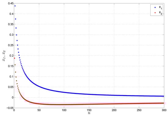
Figure 1.
The stability of the zero solution of system (28).
Example 2.
Consider the following linear incommensurate FoDS:
One can find , which leads to:
⇔
Consequently, the solution of (32) will be in the form:
where
Hence, in view of Theorem 4, system (31) is also asymptotically stable about its zero solution.
To confirm the final inference of Example 2, Figure 2 illustrates such stability by exhibiting the convergence of all system’s states to zero, which shows the validity of the proposed results.
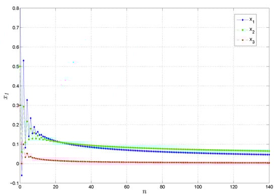
Figure 2.
The stability of the zero solution of system (31).
5. Conclusions and Future Works
In the present work, some simple applicable conditions for judging the stability of the linear incommensurate Fractional-order Difference Systems have been reported as novel results. These results have really been verified numerically by illustrating the stability of the solutions of such systems via several examples. All results of this work are applicable to be implemented in lots of difference systems, like e.g., the Duffing oscillator system which has been successfully employed to model a set of physical schemes such as beam buckling, ionization waves in plasmas, nonlinear electronic circuits, stiffening springs, and superconducting Josephson parametric amplifiers. Such investigation together with studying the dynamics of the linear incommensurate FoDSs will be some of several targets that are left for future consideration.
Author Contributions
Conceptualization, A.O.; Data curation, N.D.; Formal analysis, N.D.; Funding acquisition, G.G.; Investigation, N.D. and A.O.; Methodology, A.O.; Resources, I.M.B. and Viet-Thanh Pham; Software, I.M.B.; Validation, G.G.; Visualization, V.-T.P.; Writing—original draft, I.M.B. and V.-T.P.; Writing—review & editing, G.G. All authors have read and agreed to the published version of the manuscript.
Funding
This research received no external funding.
Conflicts of Interest
The authors declare no conflict of interest.
References
- Sun, H.; Chen, W.; Chen, Y. Variable–order fractional differential operators in anomalous diffusion modeling. Phys. Stat. Mech. Its Appl. 2009, 388, 4586–4592. [Google Scholar] [CrossRef]
- Wang, Y.; Gu, L.; Xu, Y.; Cao, X. Practical tracking control of robot manipulators with continuous fractional-order nonsingular terminal sliding mode. IEEE Trans. Ind. Electron. 2016, 63, 6194–6204. [Google Scholar] [CrossRef]
- Machado, J.; Mata, M.E. A fractional perspective to the bond graph modeling of world economies. Nonlinear Dyn. 2015, 80, 1839–1852. [Google Scholar] [CrossRef]
- Mozyrska, D.; Wyrwas, M. Stability analysis of discrete-time fractional-order Caputo-type Lorenz system. In Proceedings of the 2019 42nd International Conference on Telecommunications and Signal Processing (TSP), Budapest, Hungary, 3–5 July 2019. [Google Scholar]
- May, R.M. Simple mathematical models with very complicated dynamics. Nature 1976, 261, 459–467. [Google Scholar] [CrossRef] [PubMed]
- Diaz, J.B.; Olser, T.J. Differences of fractional order. Math. Comput. 1974, 28, 185–202. [Google Scholar] [CrossRef]
- Srivastava, H.M.; Owa, S. Univalent Functions, Fractional Calculus, and Their Applications; Ellis Horwood Ltd.: Hertfordshire, UK, 1989. [Google Scholar]
- Jarad, F.; Taş, K. On Sumudu transform method in discrete fractional calculus. Abstr. Appl. Anal. 2012, 2012, 270106. [Google Scholar] [CrossRef]
- Hilfer, R. Applications of Fractional Calculus in Physics; World Scientific Publishing Company: Singapore, 2000. [Google Scholar]
- Kilbas, A.A.; Srivastava, H.M.; Trujillo, J.J. Theory and Applications of Fractional Differential Equations; North-Holland Mathematics Studies, 204; Elsevier: Amsterdam, The Netherlands, 2006. [Google Scholar]
- Podlubny, I. Fractional Differential Equations; Academic Press: San Diego, CA, USA, 1999. [Google Scholar]
- Mozyrska, D.; Wyrwas, M. Solutions of fractional linear difference systems with Riemann–Liouville–type operator via transform method. In Proceedings of the ICFDA’14 International Conference on Fractional Differentiation and Its Applications, Catania, Italy, 23–25 June 2014. [Google Scholar]
- Mozyrska, D.; Ostalczyk, P.; Wyrwas, M. Stability conditions for fractional-order linear equations with delays. Bull. Pol. Acad. Sci. Tech. Sci. 2018, 66, 449–454. [Google Scholar]
- Mozyrska, D.; Wyrwas, M. The Z-transform method and delta type fractional difference operators. Discret. Dyn. Nat. Soc. 2015, 2015, 852734. [Google Scholar] [CrossRef]
- Abu-Saris, R.; Al-Mdallal, Q. On the asymptotic stability of linear system of fractional-order difference equations. Int. J. Theory Appl. Fract. Calc. Appl. Anal. 2013, 16, 613–629. [Google Scholar] [CrossRef]
- Mozyrska, D.; Wyrwas, M. Explicit criteria for stability of two-dimensional fractional difference systems. Int. J. Dynam. Control 2017, 5, 4–9. [Google Scholar] [CrossRef]
- Čermák, J.; Gyori, I.; Nechvátal, L. On explicit stability conditions for a linear farctional difference system. Fract. Calc. Appl. Anal. 2015, 18, 651–672. [Google Scholar] [CrossRef]
- Atici, F.M.; Eloe, P.W. Linear systems of fractional nabla difference equations. Rocky Mt. J. Math. 2011, 41, 353–370. [Google Scholar] [CrossRef]
- Chen, F. Fixed points and asymptotic stability of nonlinear fractional difference equations. El. J. Qualit. Theory Differ. Equ. 2011, 39, 1–18. [Google Scholar] [CrossRef]
- Abdeljawad, T. On Riemann and Caputo fractional differences. Comput. Math. Appl. 2011, 62, 1602–1611. [Google Scholar] [CrossRef]
- Elaydi, S.; Murakami, S. Asymptotic stability versus exponential stability in linear volterra difference equations of convolution type. J. Differ. Equ. Appl. 1996, 940, 35–46. [Google Scholar] [CrossRef]
© 2020 by the authors. Licensee MDPI, Basel, Switzerland. This article is an open access article distributed under the terms and conditions of the Creative Commons Attribution (CC BY) license (http://creativecommons.org/licenses/by/4.0/).