Finite-Time H_∞ Static Output Feedback Control for Itô Stochastic Markovian Jump Systems

Abstract

This paper focuses on the problem of finite-time $H_{\infty }$ static output feedback control for $It\widehat{o}$ stochastic systems with Markovian jumps (MJs). First of all, by introducing a new state vector and a novel signal, several sufficient conditions for the existence of static output feedback controllers are established for the considered systems with completely known transition rates (CKTRs) and partially known transition rates (PKTRs), respectively. Then the static output feedback controllers are designed via solving linear matrix inequalities (LMIs), which ensure the closed-loop systems are stochastic $H_{\infty }$ finite-time boundedness. The validity of the developed method was demonstrated through two examples.

1. Introduction

Markovian jump systems (MJs) have been investigated due to their properties in characterizing and modeling dynamic systems with random abrupt changes [1]. Up to now, much effort has been put into this field and a lot of achievements on such class of systems have been gained, for instance, stability analysis and synthesis [2], robust control and filtering [3] and sliding mode control [4]. Many results on $It\widehat{o}$ systems with Markovian jumps have been presented, for example $H_2$ control [5], Stackelberg strategy [6], $H_{-}$index in fault detection [7] and so on. However, it is well known that in practice, due to technical limitations, it is difficult to fully measure the exact value of transition rates of Markovian jump process [8]. Markovian jump system with PKTR has been paid much concerns [9]. The authors of [10] adopted a different way to solve the sequential estimation of a hidden state vector from noisy observations. Martino et al [11] designed a sequential Monte Carlo scheme by interactive parallel particle filters and applied it to urban traffic. A switching Kalman filter model was proposed in [12], where firing rates are Gaussian mixtures.

In 1961, the conception of finite-time stability was proposed by Dorato to keep system trajectories in a given threshold at a finite- time interval [13]. A great deal of results about the finite-time stability have been reported, for example, linear systems [14,15], nonlinear systems [16,17] and stochastic Itô systems [18,19,20] and so on. With regard to stochastic Itô systems, what is worth mentioning is that Kiyoshi Ito established stochastic analysis in 1944 and introduced Itô formula for calculating stochastic integral in 1951. In recent years, the research on stochastic Itô systems has become a hot spot. About the Itô stochastic MJs, the problem of finite-time stability and stabilization and finite-time guaranteed cost control had been solved in [18,19]. Liu et al [20] studied finite-time guaranteed cost control for uncertain mean-field stochastic systems.

It is worth noting that the above results are obtained through state feedback, while the system state cannot be directly measured in most cases. In addition, $H_{\infty }$ control is an important robust control design applied to eliminate the effect of disturbance [21]. In order to overcome the difficulty of state measurement and attenuate the exogenous disturbance, the research on output feedback control has been developed. Among them, static output feedback control (SOFC) has drawn the attention of a number of investigators owing to its low maintenance cost and implementation in various output feedback control schemes [22,23,24]. To be more specific, for the finite-time SOFC problem of MJs, sufficient conditions for LMIs with fixed parameter constraints are given in [22]. In recent years, stochastic $H_2/H_{\infty }$ control for MJs has become a popular area of research, in a context of partial information, the design of $H_{\infty }$, and mixed $H_2/H_{\infty }$ static output feedback controllers for Markov jump linear systems were studied [23]. Furthermore, the finite-time static output feedback $H_{\infty }$ controller was designed for Takagi–Sugeno fuzzy nonlinear systems with time-varying transition rates [24]. In [25], by introducing two new signals, sufficient conditions that the closed-loop systems are stochastic finite-time boundness with the given $H_{\infty }$ performance were obtained. From what has been discussed above, one can note that, at present, less research about static output feedback control focuses on Itô system. In this article, we will settle the issue of finite-time $H_{\infty }$ static output feedback control for Itô systems with MJs.

The paper is outlined as follows. The problem is illustrated and some useful definitions are given in Section 2. Section 3 gives the sufficient conditions such that the closed-loop Itô stochastic system is stochastic finite-time boundedness with the prescribed $H_{\infty }$ performance. In Section 4, the effectiveness of the proposed method is illustrated through two examples. Finally, Section 5 provides the conclusions.

Notation: The notations used throughout the paper are strictly standard. The transpose of M is expressed as $M^T$; $A\ge 0(A\le 0)$: A is semi-positive (negative) definite symmetric matrix; * is the symmetric hidden matrix entries; The maximum and minimum eigenvalues of the matrix M are shown by ${\lambda }_{max}\left(M\right)$ and ${\lambda }_{min}\left(M\right)$. $E\{·\}$ expresses the mathematical expectation; $He(A+B)=(A+B)+{(A+B)}^T$. For matrices, unless otherwise specified, it is assumed that they have the appropriate dimensions.

2. Problem Statement and Preliminaries

Consider linear Itô stochastic system with Markovian jumps described by

$$\begin{array}{c}\hfill \left\{\begin{array}{c}\begin{array}{cc}\hfill dx\left(t\right)& =[A\left(r_t\right)x\left(t\right)+B_1\left(r_t\right)v\left(t\right)+B_2\left(r_t\right)u\left(t\right)]dt+A_1\left(r_t\right)x\left(t\right)dW\left(t\right),\hfill \\ \hfill z\left(t\right)& =C\left(r_t\right)x\left(t\right)+D_1\left(r_t\right)v\left(t\right)+D_2\left(r_t\right)u\left(t\right),\hfill \\ \hfill y\left(t\right)& =E\left(r_t\right)x\left(t\right)+F\left(r_t\right)v\left(t\right),t\in [0,T^{*}]\hfill \end{array}\hfill \end{array}\right.\end{array}$$

(1)

where $x\left(t\right)\in R^n$, $v\left(t\right)\in R^q$, $u\left(t\right)\in R^m$, $y\left(t\right)\in R^r$ and $z\left(t\right)\in R^p$ denote the system state, the disturbance signal, control input, measured output and control output, respectively. $W\left(t\right)$ is a one-dimensional standard Brownian motion which satisfies $E\left\{dW\right(t\left)\right\}=0$ and $E\left\{dW{\left(t\right)}^2\right\}=dt$; $r_t$ is a continuous homogeneous Markovian jump process taking values in a finite state space $S=\{1,2,\cdots ,N\}$ with transition probability matrix $\Pi ={\left\{{\pi }_{ij}\right\}}_{N\times N}$ given by

$$\begin{array}{c}\hfill Pr\{r_{t+h}=j|r_t=i\}=\left\{\begin{array}{c}\begin{array}{ccc}& {\pi }_{ij}h+o\left(h\right),\hfill & i\ne j,\\ & 1+{\pi }_{ii}h+o\left(h\right),\hfill & i=j,\end{array}\hfill \end{array}\right.\end{array}$$

with $h>0$, $\underset{h\to 0}{lim}o\left(h\right)=0$, ${\pi }_{ij}$ represents the transition probability from mode i to mode j, which satisfies ${\pi }_{ij}\ge 0$ ($i\ne j$) and ${\pi }_{ii}=-{\sum }_{j=1,j\ne i}^N{\pi }_{ij}$. As a sequence, the corresponding transition probability matrix is

$${\Pi }_1=\left[\begin{array}{cccc}{\pi }_{11}& {\pi }_{12}& \cdots & {\pi }_{1N}\\ {\pi }_{21}& {\pi }_{22}& \cdots & {\pi }_{2N}\\ ⋮\\ {\pi }_{N1}& {\pi }_{N1}& \cdots & {\pi }_{NN}\end{array}\right].$$

However, it is hard to measure transition rates exactly. In this work, we also consider that the transition rates of $r_t$ is partially available. That is to say, some elements in $\Pi$ are unknown. It is assumed that the transition rate matrix $\Pi$ with two operation modes

$${\Pi }_2=\left[\begin{array}{cc}{\pi }_{11}& {\pi }_{12}\\ ?& ?\end{array}\right],$$

where ‘?’ is unknown element and ${\pi }_{ij}$ is known. All above information was covered by two sets to formulate the accessability of transition probability concisely,

$$S_k^i=\{j:if{\pi }_{ij}isknown\},$$

(2)

$$S_{uk}^i=\{j:if{\pi }_{ij}isunknown\}.$$

(3)

If $S_k^i\ne \varnothing$, then

$$S_k^i=\{k_1^i,k_2^i,\cdots ,k_l^i\},1\le l\le N,$$

where $k_l^i\in {\mathbb{N}}^{+}$, expresses as the mth known element in the mth row of matrix $\Pi$. Then let’s assume that $r_t$ and $W\left(t\right)$ are independent, and the external disturbance signal $v\left(t\right)$ satisfies

$${\int }_0^t{v}^T\left(s\right)v\left(s\right)ds<d^2,d>0.$$

To facilitate the following presentation, for $r_t=i\in S$, the ith mode system matrices can be simplified as $A_i,B_{1i},B_{2i},A_{1i},C_i,D_{1i},$ $D_{21},E_i$ and $F_i$, which are with appropriate dimension.

Now, we consider the following static output feedback controller

$$u\left(t\right)=K_{r_t}y\left(t\right),$$

(4)

where $K_{r_t}$ is an output feedback gain matrix to be designed and is given by $K_i$ for $r_t=i$. Therefore, system (1) with controller (4) can be rewritten as follows:

$$\begin{array}{c}\hfill \left\{\begin{array}{c}\begin{array}{cc}\hfill dx\left(t\right)& =[(A_i+B_{2i}{K}_i{E}_i)dt+A_{1i}dW\left(t\right)]x\left(t\right)+(B_{1i}dt+B_{2i}{K}_i{F}_{i}dt)v\left(t\right),\hfill \\ \hfill z\left(t\right)& =(C_i+D_{2i}{K}_i{E}_i)x\left(t\right)+(D_{1i}+D_{2i}{K}_i{F}_i)v\left(t\right),i\in S,t\in [0,T^{*}].\hfill \end{array}\hfill \end{array}\right.\end{array}$$

(5)

Before proceeding further, the following fundamental definitions and lemmas are introduced, which play a key role in this paper.

Definition 1

(stochastic finite-time boundedness (SFTB)). The linear Itô stochastic system (5) is said to SFTB with respect to (w.r.t) ($c_1,c_2,T^{*},R,d$), if it has an impulse-free solution in the time interval $[0,T^{*}]$ and satisfies

$$\begin{array}{c}\hfill E\left\{x^T\left(0\right)Rx\left(0\right)\right\}\le c_1\Rightarrow E\left\{x^T\left(t\right)Rx\left(t\right)\right\}<c_2,\forall t\in [0,T^{*}].\end{array}$$

holds for $R>0,c_1>0,c_2>0$ and $c_1<c_2$.

Remark 1.

When $v\left(t\right)=0$, the definition of SFTB can be reduced to stochastic finite-time stable with respect to $(c_1,c_2,T^{*},R$).

Remark 2.

Definition 1 can be interpreted as: for a given initial condition a bound and a fixed time interval, during this time interval, if state is maintained in a region of ellipsoid shape in the mean square sense, then this linear stochastic system is stochastic finite-time stable.

Definition 2

(stochastic $H_{\infty }$ finite-time boundedness( S$H_{\infty }$FTB)). The linear Itô stochastic system (5) is said to S $H_{\infty }$ FTB w.r.t ( $c_1,c_2,T^{*},R,\gamma ,d$), if under the zero initial condition, it is SFTB w.r.t ($c_1,c_2,T^{*},R,d$) and satisfies the following inequality

$$E\{{\int }_0^{T^{*}}{z}^T\left(t\right)z\left(t\right)dt\}<{\gamma }^{2}E\{{\int }_0^{T^{*}}{v}^T\left(t\right)v\left(t\right)dt\}.$$

(6)

In this article, our main target is to design a static output feedback controller (4) such that the closed-loop system (5) is S$H_{\infty }$FTB.

3. Main Results

3.1. MJS with CKTR

In this part, we give the main results through two theorems. First of all, we solve the problem of S$H_{\infty }$FTB for MJS (5) with completely known transition rate (CKTR), by introducing two new signals under the output feedback gain $K_i=J_i{P}_i^{-1}$.

Theorem 1.

For constants $\alpha ,\varphi >0$, system (5) with CKTR is S$H_{\infty }$FTB w.r.t ($c_1,c_2,T^{*},R,\gamma ,d$), if there exist matrices $J_i,P_i$, positive definite matrix $Y_i$, scalars ${\rho }_1,{\rho }_2>0$, such that the following matrix inequalities hold

$${\rho }_{1}I<{\widehat{Y}}_i^{-1}<{\rho }_{2}I$$

(7)

$$e^{\alpha T^{*}}{c}_1{\rho }_2+{\gamma }^2{d}^2-c_2{\rho }_1<0$$

(8)

$$\left[\begin{array}{ccccc}{\Theta }_{11}& {\Theta }_{12}& 0& -\varphi F_i& J_i^T{D}_{2i}^T\\ *& {\Theta }_{22}& A_{1i}{Y}_i& B_{1i}& {\Theta }_{24}\\ *& *& -Y_i& 0& 0\\ *& *& *& -{\gamma }^2{e}^{-\alpha T^{*}}I& D_{1i}^T\\ *& *& *& *& -I\end{array}\right]<0,$$

(9)

where

• ${\Theta }_{11}=-\varphi (P_i^T+P_i)$,
• ${\Theta }_{12}=\varphi (P_i{E}_i-E_i{Y}_i)+J_i^T{B}_{2i}^T$,
• ${\Theta }_{22}=He(A_i{Y}_i+B_{2i}{J}_i{E}_i)-\alpha Y_i+Y_i^T{\sum }_{j=1}^N{\pi }_{ij}{Y}_j^{-1}{Y}_i$,
• ${\Theta }_{24}=Y_i{C}_i^T+E_i^T{J}_i^T{D}_{2i}^T$,
• $Y_i^{-1}=R^{\frac{1}{2}}{\widehat{Y}}_i^{-1}{R}^{\frac{1}{2}}$.

Moreover, a expected static output feedback controller is given in the form of (4) with $K_i=J_i{P}_i^{-1}$.

Proof. 

First, define a new state vector $\mu \left(t\right)$ and a novel signal $\varrho \left(t\right)$ :

$$\begin{array}{c}\hfill \mu \left(t\right)=Y_i^{-1}x\left(t\right),\end{array}$$

(10)

$$\begin{array}{c}\hfill \varrho \left(t\right)=E_i\mu \left(t\right)-P_i^{-1}y\left(t\right).\end{array}$$

(11)

Then,

$$\begin{array}{c}\hfill V(x\left(t\right),i)=x^T\left(t\right)Y_i^{-1}x\left(t\right),\end{array}$$

(12)

where $Y_i>0$. Pre-multiplying (11) by $J_i$ results in

$$\begin{array}{c}\hfill K_{i}y\left(t\right)=J_i{E}_i\mu \left(t\right)-J_i\varrho \left(t\right).\end{array}$$

(13)

Using Schur complement, (9) is equivalent to

$$\left[\begin{array}{cccc}-\varphi (P_i^T+P_i)& \varphi (P_i{E}_i-E_i{Y}_i)+J_i^T{B}_{2i}^T& -\varphi F_i& J_i^T{D}_{2i}^T\\ *& {\Delta }_{22}& B_{1i}& Y_i{C}_i^T+E_i^T{J}_i^T{D}_{2i}^T\\ *& *& -{\gamma }^2{e}^{-\alpha T}I& D_{1i}^T\\ *& *& *& -I\end{array}\right]<0,$$

(14)

where ${\Delta }_{22}=He(A_i{Y}_i+B_{2i}{J}_i{E}_i)+{\left(A_{1i}{Y}_i\right)}^T{Y}_i^{-1}{A}_{1i}{Y}_i-\alpha Y_i+Y_i^T{\sum }_{j=1}^N{\pi }_{ij}{Y}_j^{-1}{Y}_i$. Together with (10)–(13), the closed-loop system (5) can be rewritten as

$$\begin{array}{c}\hfill \left\{\begin{array}{c}\begin{array}{cc}\hfill dx\left(t\right)& =(A_i{Y}_{i}dt+B_{2i}{J}_i{E}_{i}dt+A_{1i}{Y}_{i}d\omega )\mu \left(t\right)+B_{1i}dtv\left(t\right)-B_{2i}{J}_i\varrho \left(t\right)dt,\hfill \\ \hfill z\left(t\right)& =(C_i{Y}_i+D_{2i}{J}_i{E}_i)\mu \left(t\right)+D_{1i}v\left(t\right)-D_{2i}{J}_i\varrho \left(t\right).\hfill \end{array}\hfill \end{array}\right.\end{array}$$

Pre-multiplying (11) by $P_i$, we can get the following equation associated with $\varrho \left(t\right)$, $\mu \left(t\right)$ and $v\left(t\right)$

$${\varsigma }_i=(P_i{E}_i-E_i{Y}_i)\mu \left(t\right)-F_{i}v\left(t\right)-P_i\varrho \left(t\right)=0.$$

Defining $\xi$ as the weak infinitesimal operator, and using Itô’s formula, (6) will satisfy if

$$\xi V(x\left(t\right),i)-\alpha V(x\left(t\right),i)-{\gamma }^2{e}^{-\alpha T^{*}}{v}^T\left(t\right)v\left(t\right)+z^T\left(t\right)z\left(t\right)<0.$$

(15)

To this end, pre and post-multiplying (14) by $\Phi$ and ${\Phi }^T$, we can obtain

$$\Phi \left[\begin{array}{cccc}-\varphi (P_i^T+P_i)& \varphi (P_i{E}_i-E_i{Y}_i)+J_i^T{B}_{2i}^T& -\varphi F_i& J_i^T{D}_{2i}^T\\ *& {\Delta }_{22}& B_{1i}& Y_i{C}_i^T+E_i^T{J}_i^T{D}_{2i}^T\\ *& *& -{\gamma }^2{e}^{-\alpha T^{*}}I& D_{1i}^T\\ *& *& *& -I\end{array}\right]{\Phi }^T<0,$$

(16)

where

• $\Phi =\left[\varrho \right(t\left)\mu \right(t\left)v\right(t\left)z\right(t\left)\right]$,
• ${\Delta }_{22}=He(A_i{Y}_i+B_{2i}{J}_i{E}_i)+{\left(A_{1i}{Y}_i\right)}^T{Y}_i^{-1}\left(A_{1i}{Y}_i\right)-\alpha Y_i++Y_i^T{\sum }_{j=1}^N{\pi }_{ij}{Y}_j^{-1}{Y}_i$,
• $Y_i^{-1}=R^{\frac{1}{2}}{\widehat{Y}}_i^{-1}{R}^{\frac{1}{2}}$.

We can see that (16) is equivalent to

$$\begin{array}{c}\xi V(x\left(t\right),i)-\alpha V(x\left(t\right),i)-{\gamma }^2{e}^{-\alpha T^{*}}{v}^T\left(t\right)v\left(t\right)+2\varphi {\varrho }^T\left(t\right){\varsigma }_i+z^T\left(t\right)z\left(t\right)<0.\hfill \end{array}$$

Therefore, (15) holds.

By (15), we can get

$$\xi V(x\left(t\right),i)-\alpha V(x\left(t\right),i)-{\gamma }^2{e}^{-\alpha T^{*}}{v}^T\left(t\right)v\left(t\right)<0,$$

(17)

then, taking the mathematical expectation of (17), we have

$$E\left\{\xi e^{-\alpha t}V(x\left(t\right),i)\right\}<{\gamma }^2{e}^{-\alpha (t+T^{*})}E\left\{v^T\left(t\right)v\left(t\right)\right\},$$

(18)

integrating both sides of (18) from 0 to t, with $t\in [0,T^{*}]$, it can be deduced that

$$\begin{array}{c}{e}^{-\alpha t}E\left\{V(x\left(t\right),i)\right\}<E\left\{V(x\left(0\right),r_0)\right\}+{\gamma }^{2}E\left\{{\int }_0^t{e}^{-\alpha (\tau +T^{*})}{v}^T\left(\tau \right)v\left(\tau \right)d\tau \right\},\hfill \end{array}$$

(19)

pre-multiplying (19) by $e^{\alpha t}$, it is easy to see

$$\begin{array}{c}\hfill \begin{array}{cc}\hfill E\left\{V\right(x\left(t\right),i\left)\right\}& <e^{\alpha t}E\left\{V(x\left(0\right),r_0)\right\}+{\gamma }^2{d}^2<e^{\alpha T^{*}}{\rho }_{max}\left({\widehat{Y}}_i^{-1}\right)x^T\left(0\right)Rx\left(0\right)+{\gamma }^2{d}^2\hfill \\ & \le e^{\alpha T^{*}}{\rho }_{max}\left({\widehat{Y}}_i^{-1}\right)c_1+{\gamma }^2{d}^2.\hfill \end{array}\end{array}$$

Since

$$E\left\{V(x\left(t\right),i)\right\}\ge {\rho }_{min}\left({\widehat{Y}}_i^{-1}\right)E\left\{x^T\left(t\right)Rx\left(t\right)\right\},$$

it can be verified that

$$E\left\{x^T\left(t\right)Rx\left(t\right)\right\}<\frac{e^{\alpha T^{*}}{\rho }_{max}\left({\widehat{Y}}_i^{-1}\right)c_1+{\gamma }^2{d}^2}{{\rho }_{min}\left({\widehat{Y}}_i^{-1}\right)},$$

it follows that from (8),

$$E\left\{x^T\left(t\right)Rx\left(t\right)\right\}<\frac{e^{\alpha T^{*}}{\rho }_{max}\left({\widehat{Y}}_i^{-1}\right)c_1+{\gamma }^2{d}^2}{{\rho }_{min}\left({\widehat{Y}}_i^{-1}\right)}<c_2.$$

From Definition 1, system (5) with CKTR is SFTB.

Multiplying (15) with $e^{-\alpha t}$ and taking mathematical expectation

$$E\left\{\zeta \left[e^{-\alpha t}V(x\left(t\right),i)\right]\right\}<E\left\{e^{-\alpha t}[{\gamma }^2{e}^{-\alpha T^{*}}{v}^T\left(t\right)v\left(t\right)-z^T\left(t\right)z\left(t\right)]\right\},$$

(20)

integrating (20) from 0 to t, the result follows

$$E\{{\int }_0^t{e}^{-\alpha \hslash }[z^T(\hslash )z(\hslash )-{\gamma }^2{e}^{-\alpha T^{*}}{v}^T(\hslash )v(\hslash )]d\hslash \}<0.$$

For all $t\in [0,T^{*}]$ , it implies that

$$\begin{array}{c}\hfill \begin{array}{cc}\hfill E\{{\int }_0^{T^{*}}{z}^T\left(t\right)z\left(t\right)dt\}& \le e^{-\alpha T^{*}}E\{{\int }_0^{T^{*}}{e}^{-\alpha t}{z}^T\left(t\right)z\left(t\right)dt\}<e^{\alpha T^{*}}E\{{\int }_0^{T^{*}}{\gamma }^2{e}^{-\alpha (t+T^{*})}{v}^T\left(t\right)v\left(t\right)dt\}\hfill \\ & <{\gamma }^{2}E\{{\int }_o^T{v}^T\left(t\right)v\left(t\right)dt\}.\hfill \end{array}\end{array}$$

From the above, the closed-loop system (5) with CKTR is S$H_{\infty }$FTB with the proposed static output feedback controller. □

Remark 3.

By the introducing $\mu \left(t\right)$ and $\varrho \left(t\right)$, we can decouple the connection between input matrix and output matrix. We use a zero term ${\varsigma }_i$ to make the conditions given in Theorem 1 solvable via linear matrix inequalities.

Considering another form of the output feedback gain matrix $K_i=Q_i^{-1}{L}_i$, and the corresponding theorem is given as follows.

Theorem 2.

Given positive scalars β and φ, system (5) with CKTR is S$H_{\infty }$FTB w.r.t ($c_1,c_2,T^{*},R,\gamma ,d$), if there exist matrices $Q_i,L_i$, and positive definite matrices $X_i(i\in S)$, scalars ${\rho }_1,{\rho }_2>0$ satisfying

$${\rho }_{1}R<X_i<{\rho }_{2}R,$$

$$e^{\beta T^{*}}{c}_1{\rho }_2+{\gamma }^2{d}^2-c_2{\rho }_1<0,$$

$$\left[\begin{array}{cccc}{\Xi }_{11}& {\Xi }_{12}& L_i{F}_i& \phi D_{2i}^T\\ *& {\Xi }_{22}& {\Xi }_{23}& C_i^T\\ *& *& -{\gamma }^2{e}^{-\beta T^{*}}I& D_{1i}^T\\ *& *& *& -I\end{array}\right]<0,$$

(21)

where

• ${\Xi }_{11}=-\phi (Q_i^T+Q_i)$,
• ${\Xi }_{12}=\phi {(X_i{B}_{2i}-B_{2i}{Q}_i)}^T+L_i{E}_i$,
• ${\Xi }_{22}=He(A_i{X}_i+B_{2i}{L}_i{E}_i)+A_{1i}^T{X}_i{A}_{1i}-\beta X_i+{\sum }_{j=1}^N{\pi }_{ij}{X}_j$,
• ${\Xi }_{23}=X_i{B}_{1i}+B_{2i}{L}_i{F}_i$, Beyond that,

  $$K_i=Q_i^{-1}{L}_i.$$

Proof. 

Set $\mu \left(t\right)=x\left(t\right)$ and $\varrho \left(t\right)={\phi }^{-1}u\left(t\right)$ and construct the following function

$$V(x\left(t\right),i)=x^T\left(t\right)X_{i}x\left(t\right),$$

where $X_i>0$.

By $K_i=Q_i^{-1}{L}_i$, multiply $u\left(t\right)=K_{i}y\left(t\right)$ from the left by $Q_i$, one has

$${\varsigma }_i=L_i{E}_{i}x\left(t\right)+L_i{F}_{i}v\left(t\right)-Q_{i}u\left(t\right)=0.$$

Then, (1) is described

$$\begin{array}{c}\hfill \begin{array}{cc}\hfill dx\left(t\right)=& A_{i}x\left(t\right)dt+B_{1i}v\left(t\right)dt+(B_{2i}-X_i^{-1}{B}_{2i}{Q}_i)u\left(t\right)dt+A_{1i}x\left(t\right)d\omega \hfill \\ & +X_i^{-1}(B_{2i}{L}_i{E}_{i}x\left(t\right)+B_{2i}{L}_i{F}_{i}v\left(t\right))dt.\hfill \end{array}\end{array}$$

(22)

Pre-multiplying (22) by $X_i$, we can get

$$\begin{array}{c}\hfill \begin{array}{cc}\hfill X_{i}dx\left(t\right)=& (X_i{A}_{i}dt+X_i{A}_{1i}d\omega +B_{2i}{L}_i{E}_{i}dt)x\left(t\right)+(X_i{B}_{1i}dt+B_{2i}{L}_i{F}_{i}dt)v\left(t\right)\hfill \\ & +\phi (X_i{B}_{2i}dt-B_{2i}{Q}_{i}dt)\varrho \left(t\right).\hfill \end{array}\end{array}$$

According to Definition 2, we prove that the following inequality holds

$$E\{\zeta V(x\left(t\right),i)-\beta V(x\left(t\right),i)-{\gamma }^2{e}^{-\beta T^{*}}{v}^T\left(t\right)v\left(t\right)+z^T\left(t\right)z\left(t\right)\}<0.$$

(23)

By taking a similar approach to Theorem 1, (21) can be rewritten as

$$E\{\zeta V(x\left(t\right),i)-\beta V(x\left(t\right),i)+2{\xi }^T\left(t\right){\varsigma }_i-{\gamma }^2{e}^{-\beta T^{*}}{v}^T\left(t\right)v\left(t\right)+z^T\left(t\right)z\left(t\right)\}<0.$$

(24)

It is easy to see that (24) is correct from (23).

Then, using the same method as Theorem 1, we can easily prove that the closed-loop system (5) with CKTR is S$H_{\infty }$FTB with the output feedback gain matrix $K_i=Q_i^{-1}{L}_i$. □

3.2. MJS with PKTR

The following theorems will give a sufficient condition of S$H_{\infty }$FTB for system (5) with PKTR.

Theorem 3.

Given positive scalars α and ϕ, system (5) with PKTR is S$H_{\infty }$FTB w.r.t ($c_1,c_2,T^{*},R,\gamma ,d$), if there exist matrices ${\tilde{J}}_i,{\tilde{P}}_i$, positive definite matrice $Y_i$, two positive scalars ${\rho }_1,{\rho }_2$, satisfying

$${\rho }_{1}I<{\widehat{Y}}_i^{-1}<{\rho }_{2}I,$$

$$e^{\alpha T^{*}}{c}_1{\rho }_2+{\gamma }^2{d}^2-c_2{\rho }_1<0,$$

$$\left[\begin{array}{ccccc}-\varphi ({\tilde{P}}_i^T+{\tilde{P}}_i)& \varphi ({\tilde{P}}_i{E}_i-E_i{Y}_i)+{\tilde{J}}_i^T{B}_{2i}^T& 0& -\varphi F_i& {\tilde{J}}_i^T{D}_{2i}^T\\ *& {\Lambda }_{22}& A_{1i}{Y}_i& B_{1i}& Y_i{C}_i^T+E_i^T{\tilde{J}}_i^T{D}_{2i}^T\\ *& *& -Y_i& 0& 0\\ *& *& *& -{\gamma }^2{e}^{-\alpha T^{*}}I& D_{1i}^T\\ *& *& *& *& -I\end{array}\right]<0,$$

(25)

where

• ${\Omega }_j=He(A_i{Y}_i+B_{2i}{\tilde{J}}_i{E}_i)$,
• ${\Lambda }_{22}=(1+Y_i^T{\sum }_{j\in S_k^i}{\pi }_{ij}){\Omega }_j+Y_i^T{\sum }_{j\in S_k^i}{\pi }_{ij}{Y}_j^{-1}{Y}_i+Y_i^T{\sum }_{j\in S_{uk}^i}{\pi }_{ij}({\Omega }_j+Y_j^{-1})-\alpha Y_i$,
• $Y_i^{-1}=R^{\frac{1}{2}}{\widehat{Y}}_i^{-1}{R}^{\frac{1}{2}}$.

The static output feedback controller gain is given by $K_i={\tilde{J}}_i{\tilde{P}}_i^{-1}$.

Proof. 

Using Schur complement, (25) is equivalent to

$$\left[\begin{array}{cccc}-\varphi ({\tilde{P}}_i^T+{\tilde{P}}_i)& \varphi ({\tilde{P}}_i{E}_i-E_i{Y}_i)+{\tilde{J}}_i^T{B}_{2i}^T& -\varphi F_i& {\tilde{J}}_i^T{D}_{2i}^T\\ *& {{\rm Y}}_{22}& B_{1i}& Y_i{C}_i^T+E_i^T{\tilde{J}}_i^T{D}_{2i}^T\\ *& *& -{\gamma }^2{e}^{-\alpha T}I& D_{1i}^T\\ *& *& *& -I\end{array}\right]<0,$$

where

$${{\rm Y}}_{22}=(1+Y_i^T\sum _{j\in S_k^i}{\pi }_{ij}){\Omega }_j+{(A_{1i}{Y}_i)}^T{Y}_i^{-1}{A}_{1i}{Y}_i+Y_i^T\sum _{j\in S_k^i}{\pi }_{ij}{Y}_j^{-1}{Y}_i+Y_i^T\sum _{j\in S_{uk}^i}{\pi }_{ij}({\Omega }_j+Y_j^{-1})-\alpha Y_i.$$

Because of ${\sum }_{j=1}^N{\pi }_{ij}=0$, then

$${\Delta }_{22}={\Omega }_j+{\left(A_{1i}{Y}_i\right)}^T{Y}_i^{-1}\left(A_{1i}{Y}_i\right)-\alpha Y_i+Y_i^T{\sum }_{j=1}^N{\pi }_{ij}{Y}_j^{-1}{Y}_i+Y_i^T{\sum }_{j=1}^N{\pi }_{ij}{\Omega }_j$$

.

Together with (2) and (3),

$$\begin{array}{c}\hfill \begin{array}{cc}\hfill {\Delta }_{22}=& {\Omega }_j+{\left(A_{1i}{Y}_i\right)}^T{Y}_i^{-1}\left(A_{1i}{Y}_i\right)+Y_i^T\sum _{j\in S_k^i}{\pi }_{ij}{Y}_j^{-1}{Y}_i+Y_i^T\sum _{j\in S_{uk}^i}{\pi }_{ij}{Y}_j^{-1}{Y}_i\hfill \\ & +Y_i^T\sum _{j\in S_k^i}{\pi }_{ij}{\Omega }_j+Y_i^T\sum _{j\in S_{uk}^i}{\pi }_{ij}{\Omega }_j-\alpha Y_i\hfill \\ \hfill =& (1+Y_i^T\sum _{j\in S_k^i}{\pi }_{ij}){\Omega }_j+{\left(A_{1i}{Y}_i\right)}^T{Y}_i^{-1}\left(A_{1i}{Y}_i\right)+Y_i^T\sum _{j\in S_k^i}{\pi }_{ij}{Y}_j^{-1}{Y}_i+Y_i^T\sum _{j\in S_{uk}^i}{\pi }_{ij}({\Omega }_j+Y_j^{-1})-\alpha Y_i.\hfill \end{array}\end{array}$$

The rest of proof is similar to Theorem 1, so it is omitted. □

Considering another form of the output feedback gain matrix $K_i={\tilde{Q}}_i^{-1}{\tilde{L}}_i$, and alternative theorem is presented below.

Theorem 4.

The closed-loop system (5) with PKTR is S$H_{\infty }$FTB w.r.t ($c_1,c_2,T^{*},R,\gamma ,d$), if there exist matrices ${\tilde{Q}}_i,{\tilde{L}}_i$, and positive definite matrice $X_i(i\in S)$, two positive scalars ${\rho }_1,{\rho }_2$ and given positive scalars β and φ, satisfying

$${\rho }_{1}R<X_i<{\rho }_{2}R,$$

$$e^{\beta T^{*}}{c}_1{\rho }_2+{\gamma }^2{d}^2-c_2{\rho }_1<0,$$

$$\left[\begin{array}{cccc}-\phi ({\tilde{Q}}_i^T+{\tilde{Q}}_i)& \phi {(X_i{B}_{2i}-B_{2i}{\tilde{Q}}_i)}^T+{\tilde{L}}_i{E}_i& L_i{F}_i& \phi D_{2i}^T\\ *& {\Delta }_{22}& X_i{B}_{1i}+B_{2i}{\tilde{L}}_i{F}_i& C_i^T\\ *& *& -{\gamma }^2{e}^{-\beta T^{*}}I& D_{1i}^T\\ *& *& *& -I\end{array}\right]<0,$$

where

$$\begin{array}{cc}\hfill {\Delta }_{22}=& (1+\sum _{j\in S_k^i}{\pi }_{ij})He(A_i{X}_i+B_{2i}{\tilde{L}}_i{E}_i)+A_{1i}^T{X}_i{A}_{1i}+\sum _{j\in S_k^i}{\pi }_{ij}{X}_j\hfill \\ & +\sum _{j\in S_{uk}^i}{\pi }_{ij}[He(A_i{X}_i+B_{2i}{\tilde{L}}_i{E}_i)+X_j]-\beta X_i.\hfill \end{array}$$

The static output feedback controller gain is given by $K_i={\tilde{Q}}_i^{-1}{\tilde{L}}_i.$

Remark 4.

It is not easy to deal with the condition (7) and (8) by applying LMIs. To address this problem, set ${\widehat{Y}}_i^{-1}$ with $I<{\widehat{Y}}_i^{-1}<{\delta }^{-1}I$ and $Y_i^{-1}=R^{\frac{1}{2}}{\widehat{Y}}_i^{-1}{R}^{\frac{1}{2}}$, then (7) and (8) can be replaced with following constraints

$$\delta R^{-1}<Y_i^{-1}<R^{-1},$$

(26)

$$\left[\begin{array}{cc}{e}^{-\alpha T}(-c_2+{\gamma }^2{d}^2)& \sqrt{c_1}\\ \sqrt{c_1}& -\delta I\end{array}\right]<0.$$

(27)

Through this transformation, the static output controller can be calculated by LMIs (26), (27) and (9) or (25).

Remark 5.

The conditions given in Theorem 1 can be transformed into the problem as follows

$$\begin{array}{c}\hfill \begin{array}{cc}& min{c}_2^2+{\gamma }^2\hfill \\ & s.t.\left(26\right),\left(27\right),\left(9\right).\hfill \end{array}\end{array}$$

(28)

Remark 6.

The work of static output feedback control problem in deterministic systems has been studied by Shen M et al. [25], and this paper investigates the static output feedback control problem of Itô stochastic system through Theorems 1 and 2. In addition, compared with [25], this paper also studies the S$H_{\infty }$FTB for system (5) with partially known transition rates in Theorems 3 and 4.

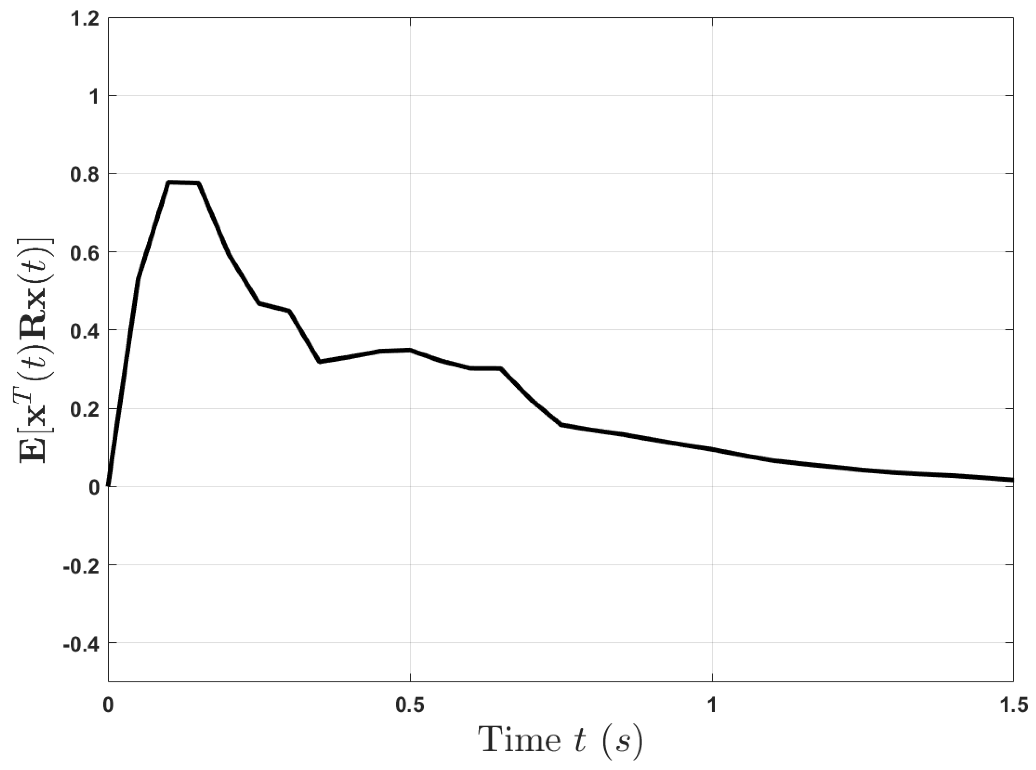
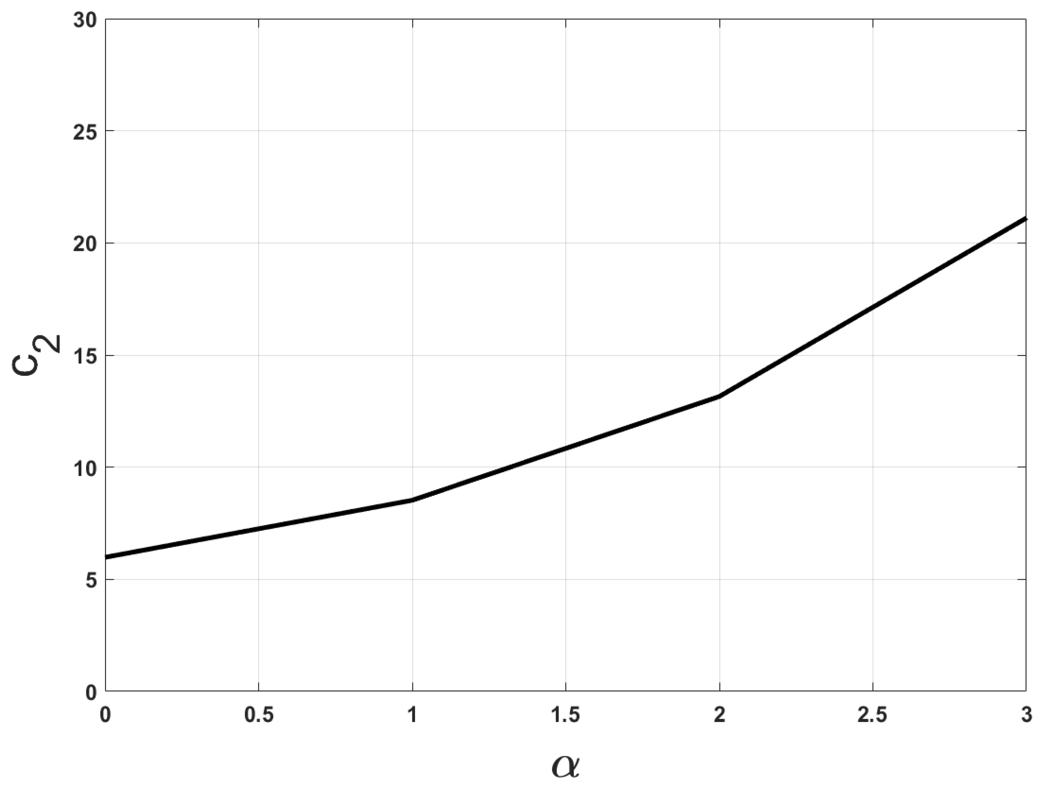
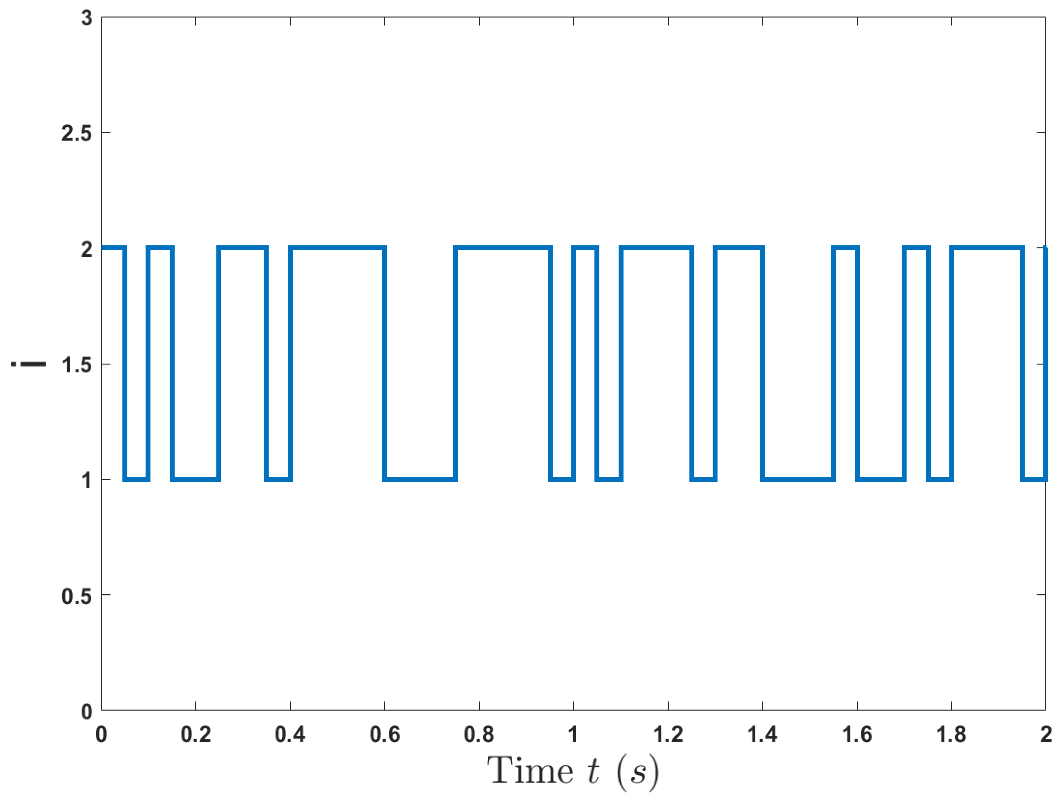
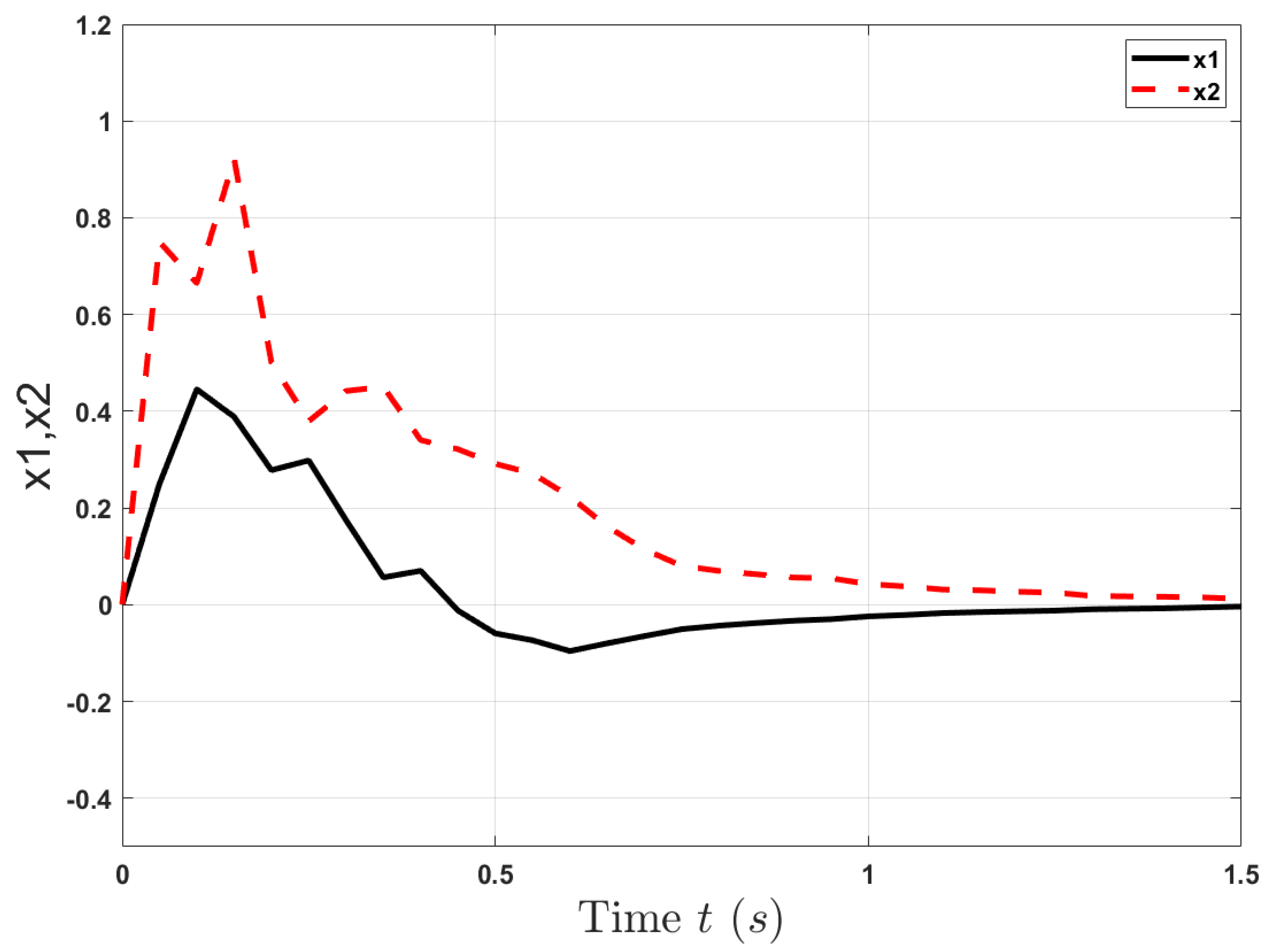
4. Numerical Examples

Simulations of two examples are presented in this section to verify the effectiveness and applicability of the proposed method in this paper.

Example 1.

Consider system (5) with two modes and the transition probability is completely known.

Mode 1:

• $A_1=\left[\begin{array}{cc}-3& 1\\ -2& -5\end{array}\right],A_{11}=\left[\begin{array}{cc}2.1& 0.9\\ 1.5& 1.8\end{array}\right],B_{11}=\left[\begin{array}{c}2\\ 1\end{array}\right],B_{21}=\left[\begin{array}{c}1\\ 1\end{array}\right],C_1=\left[\begin{array}{cc}-1& 0\\ 0& 1\end{array}\right],$
• $D_{11}=\left[\begin{array}{c}0.2\\ 0.2\end{array}\right],D_{21}=\left[\begin{array}{c}0.4\\ 0.2\end{array}\right],E_1=\left[\begin{array}{cc}-1& 0\\ 0& 1\end{array}\right],F_1=\left[\begin{array}{c}0.1\\ 0.1\end{array}\right].$

Mode 2:

• $A_2=\left[\begin{array}{cc}-5& -2\\ 4& -1\end{array}\right],A_{12}=\left[\begin{array}{cc}2.1& 1.1\\ 1& 1.2\end{array}\right],B_{12}=\left[\begin{array}{c}1\\ 3\end{array}\right],B_{22}=\left[\begin{array}{c}1\\ 1\end{array}\right],C_2=\left[\begin{array}{cc}1& 0\\ 0& 1\end{array}\right],$
• $D_{12}=\left[\begin{array}{c}0.2\\ 0.3\end{array}\right],D_{22}=\left[\begin{array}{c}0.3\\ 0.5\end{array}\right],E_2=\left[\begin{array}{cc}-0.5& 0\\ 0& 0.5\end{array}\right],F_2=\left[\begin{array}{c}0.1\\ 0.1\end{array}\right].$

The transiting between the two modes is

• ${\Pi }_1=\left[\begin{array}{cc}-0.3& 0.3\\ 0.35& -0.35\end{array}\right].$

The external disturbance $v\left(t\right)=\frac{0.1}{1+t^2}$. One possible mode evolution is given in Figure 1.

Given $\alpha =1,c_1=0.6,T^{*}=1,d=2,R=I,x_0={\left[00\right]}^T$. With the help of MATLAB, from Theorem 1, it yields that $c_2=11.064,\gamma =3.820({ϵ}_1=1,{ϵ}_2=1)$. The static output feedback gains are calculated as follows:

$K_1=\left[\begin{array}{cc}-0.3238& -0.5388\end{array}\right],K_2=\left[\begin{array}{cc}0.0322& -0.0287\end{array}\right].$

With these conditions, we can obtain the state response curves of closed-loop system (5) in Figure 2 and the simulated curves of $E\left[x^T\left(t\right)Rx\left(t\right)\right]$ in Figure 3. From Figure 2 and Figure 3, we can see that (5) with CKTR is S$H_{\infty }$FTB.

It should note that the optimization problem (28) relies on the parameter $\alpha$, once the value of $\alpha$ is determined, we can treat (28) as a linear matrix inequality. By using the linear search algorithm, we can find feasible solution when $0\le \alpha \le 3$. Figure 4 and Figure 5 show the optimal value with different value of $\alpha$.

Example 2.

Consider system (5) with two modes, and the transition probability is partially known. In this case, the system parameters of Example 1 are used. The transition probability matrix between the two modes is

• ${\Pi }_2=\left[\begin{array}{cc}-1.2& 1.2\\ ?& ?\end{array}\right]$.

By using the relevant data from Example 1: $\alpha =1,c_1=0.6,T^{*}=1,d=2,R=I,x_0={\left[00\right]}^T$, from Theorem 3, we have $c_2=11.064,\gamma =3.820({ϵ}_1=1,{ϵ}_2=1),$ the static output feedback gains

$K_1=\left[\begin{array}{cc}-0.3238& -0.5388\end{array}\right],K_2=\left[\begin{array}{cc}0.0322& -0.0287\end{array}\right]$.

For the simulation purpose, it is assumed that the actual partially unknown transition rate matrix is

• ${\Pi }_1=\left[\begin{array}{cc}-1.2& 1.2\\ 0.5& -0.5\end{array}\right].$

In this case, we can get another possible Markov mode evolution Figure 6. Meanwhile, Figure 7 and Figure 8 are the simulated curves of $E\left[x^T\left(t\right)Rx\left(t\right)\right]$ and the state response curves of system (5), which show that MJS (5) with partially known transition rates is S$H_{\infty }$FTB.

5. Conclusions

In this paper, the problem of finite-time $H_{\infty }$ static output feedback control for $It\widehat{o}$ stochastic systems with Markovian jump has been studied. By introducing a new state vector and a novel signal, several new sufficient conditions are presented for the considered system with completely known or partially unknown transition rates to be S$H_{\infty }$FTB. At last, the validity of proposed methods is verified by two numerical examples.

References

1. Costa, O.L.V.; Fragoso, M.D.; Todorov, M.G. Continuous-Time Markov Jump Linear Systems; Springer: Berlin/Heidelberg, Germany, 2013. [Google Scholar]
2. Zhang, L.; Lam, J. Necessary and sufficient conditions for analysis and synthesis of Markov jump linear systems with incomplete transition descriptions. IEEE Trans. Autom. Control. 2010, 55, 1695–1701. [Google Scholar] [CrossRef] [Green Version]
3. Hua, M.; Zhang, L.; Yao, F. Robust H filtering for continuous-time nonhomogeneous Markov jump nonlinear systems with randomly occurring uncertainties. Signal Process. 2018, 148, 250–259. [Google Scholar] [CrossRef]
4. Li, H.; Shi, P.; Wu, L. Observer-based adaptive sliding mode control for nonlinear Markovian jump systems. Automatica 2016, 64, 133–142. [Google Scholar] [CrossRef]
5. Stadtmann, F.; Costa, O.L.V. H2 control of continuous-time hidden Markov jump linear systems. IEEE Trans. Autom. Control. 2017, 62, 4031–4037. [Google Scholar] [CrossRef]
6. Hukaidani, H.; Xu, H.; Shima, T.; Dragan, V. A stochastic multiple-leader-follower incentive Stackelberg strategy for Markov jump linear systems. IEEE Control Syst. Lett. 2017, 1, 250–255. [Google Scholar] [CrossRef]
7. Liu, X.; Zhang, W.; Li, Y. Hindex for continuous-time stochastic systems with Markov jump and multiplicative noise. Automatica 2019, 105, 167–178. [Google Scholar] [CrossRef]
8. Du, B.; Lam, J.; Zou, Y.; Zhan, S. Stability and stabilization for Markovian jump time-delay systems with partially unknown transition rates. IEEE Trans. Circ. Syst. 2013, 62, 341–351. [Google Scholar] [CrossRef] [Green Version]
9. Li, X.; Lam, J.; Gao, H.; Xiong, J. H and H2 filtering for linear systems with uncertain Markov transition. Automatica 2016, 67, 252–266. [Google Scholar] [CrossRef]
10. Caron, F.; Davy, M.; Duflos, E. Particle filtering for multisensor data fusion with switching observation models: Application to land vehicle positioning. IEEE Trans. Signal Process. 2007, 55, 2703–2719. [Google Scholar] [CrossRef]
11. Martino, L.; Read, J.; Elvira, V.; Louzada, F. Cooperative parallel particle filters for on-line model selection and Applications to urban mobility. Digit. Signal Process. 2017, 60, 172–185. [Google Scholar] [CrossRef] [Green Version]
12. Wu, W.; Black, M.J.; Mumford, D.; Gao, Y.; Bienenstock, E.; Donoghue, J.P. Modeling and decoding motor cortical activity using a switching Kalman filter. IEEE Trans. Biomed. Eng. 2004, 51, 933–942. [Google Scholar] [CrossRef] [Green Version]
13. Dorato, P. Short time stability in linear time-varying systems. In Proceedings of the IRE International Convention Record Part 4, New York, NY, USA, 26 October 1961; pp. 83–87. [Google Scholar]
14. Amato, F.; Ariola, M.; Cosentino, C. Finite-time stability of linear time-varying systems: Analysis and controller design. IEEE Trans. Autom. Control 2010, 55, 1003–1008. [Google Scholar] [CrossRef]
15. Amato, F.; Darouach, M.; Tommasi, G. Finite-time stabilization, detectability, and dynamic output feedback finite-time stabilization of linear systems. IEEE Trans. Autom. Control 2017, 62, 6521–6528. [Google Scholar] [CrossRef]
16. Amato, F.; Cosentino, C.; Merola, A. Sufficient conditions for finite-time stability and stabilization of nonlinear quadratic systems. IEEE Trans. Autom. Control 2010, 55, 430–434. [Google Scholar] [CrossRef]
17. Zhang, Y.; Shi, Y.; Shi, P. Resilient and robust finite-time H control for uncertain discrete-time jump nonlinear systems. Appl. Math. Model. 2017, 49, 612–629. [Google Scholar] [CrossRef]
18. Yan, Z.; Zhang, W.; Zhang, G. Finite-time stability and stabilization of Itô stochastic systems with Markovian switching: Mode-dependent parameter approach. IEEE Trans. Autom. Control 2015, 60, 2428–2433. [Google Scholar] [CrossRef]
19. Yan, Z.; Park, J.; Zhang, W. Finite-time guaranteed cost control for Itô stochastic Markovian jump systems with incomplete transition rates. Int. J. Robust Nonlinear Control 2017, 27, 66–83. [Google Scholar] [CrossRef]
20. Liu, X.; Liu, Q.; Li, Y. Finite-time guaranteed cost control for uncertain mean-field stochastic systems. J. Frankl. Inst. 2020, 57, 2813–2829. [Google Scholar] [CrossRef]
21. Hinrichsen, D.; Pritchard, A. Stochastic H. Siam J. Control Optim. 1998, 36, 1504–1538. [Google Scholar] [CrossRef]
22. Zhang, Y.; Liu, C.; Mu, X. Robust finite-time H control of singular stochastic systems via static output feedback. Appl. Math. Comput. 2012, 218, 5629–5640. [Google Scholar] [CrossRef]
23. Oliveira, A.; Costa, O.; Daafouz, J. Suboptimal H2 and H static output feedback control of hidden Markov jump linear systems. Eur. J. Control 2020, 51, 10–18. [Google Scholar] [CrossRef]
24. Wang, J.; Ma, S.; Zhang, C. Finite-time H control for T-S fuzzy descriptor semi-Markov jump systems via static output feedback. Fuzzy Sets Syst. 2019, 365, 60–80. [Google Scholar] [CrossRef]
25. Shen, M.; Yan, S.; Zhang, G.; Park, J. Finite-time H static output control of Markov jump systems with an auxiliary approach. Math. Comput. 2016, 273, 553–561. [Google Scholar] [CrossRef]
Figure 1. One possible Markov mode evolution.
Mathematics 08 01709 g001
Figure 2. The response of system (5).
Mathematics 08 01709 g002
Figure 3. The trajectory of E [ x T ( t ) R x ( t ) ] .
Mathematics 08 01709 g003
Figure 4. The local optimal bound of c 2 when α [ 0 , 3 ] .
Mathematics 08 01709 g004
Figure 5. The local optimal bound of γ when α [ 0 , 3 ] .
Mathematics 08 01709 g005
Figure 6. Another possible Markov mode evolution.
Mathematics 08 01709 g006
Figure 7. State response curves of closed-loop system.
Mathematics 08 01709 g007
Figure 8. The trajectory of E [ x T ( t ) R x ( t ) ] .
Mathematics 08 01709 g008