Estimation in Partial Functional Linear Spatial Autoregressive Model

Abstract

Functional regression allows for a scalar response to be dependent on a functional predictor; however, not much work has been done when response variables are dependence spatial variables. In this paper, we introduce a new partial functional linear spatial autoregressive model which explores the relationship between a scalar dependence spatial response variable and explanatory variables containing both multiple real-valued scalar variables and a function-valued random variable. By means of functional principal components analysis and the instrumental variable estimation method, we obtain the estimators of the parametric component and slope function of the model. Under some regularity conditions, we establish the asymptotic normality for the parametric component and the convergence rate for slope function. At last, we illustrate the finite sample performance of our proposed methods with some simulation studies.

1. Introduction

Over the last two decades, there has been an increasing interest in functional data analysis in econometrics, biometrics, chemometrics, and medical research, as well as other fields. Due to the infinite-dimensional nature of functional data, the classical methods for functional data are no longer applicable. There has been a large amount of work in function data analysis; see Ramsay and Silverman [1], Cardot et al. [2], Yao et al. [3], Lian and Li [4], Fan et al. [5], Feng and Xue [6], Kong et al. [7], and Yu et al. [8]. Some methods and theories on partial functional linear models have been proposed. For example, based on a two-stage nonparametric regression calibration method, Zhang et al. [9] discussed a partial functional linear model. Shin [10] proposed new estimators of the parameters and coefficient function of partial functional linear model. Lu et al. [11] considered quantile regression for the functional partially linear model. Yu et al. [12] proposed a prediction procedure for the partial functional linear quantile regression model. However, the aforementioned articles have a significant limitation. That is, they assumed that response variables are independence variables. However, in many fields, such as economics, finance, and environmental studies, sometimes response variables are dependence spatial variables. Therefore, it is of practical interest to develop more flexible approaches using a broader family of data.

There has been considerable work on dependence spatial variables. One useful approach in dealing with spatial dependence is the spatial autoregressive model, which adds a weighted average of nearby values of the dependent variable to the base set of explanatory variables. Theories and methods based on parametric spatial autoregressive models have been extensively studied in Cliff and Ord [13], Anselin [14], and Cressie [15]. Lee [16] proposed the quasi-maximum likelihood estimation. Then, Su and Jin [17] extended the quasi-likelihood estimation method to partially linear spatial autoregressive models. Koch and Krisztin [18] developed the B-splines and genetic-algorithms method for partially linear spatial autoregressive models. Chen et al. [19] proposed a new estimation method based on the kernel estimation method. Du et al. [20] considered partially linear additive spatial autoregressive models, proposed the instrumental variable estimation method, and established the asymptotic normality for the parametric component.

It is a good idea to develop more flexible approaches using a broader family of data, where the limitation can, in principle, be easily solved by proposing a new model. Thus, in this paper, based on spatial variables and functional data, we combine the spatial autoregressive model and the partial functional linear model, and propose a partial functional linear spatial autoregressive model.

Let $Y_i$ be a real-valued dependence spatial variable corresponding to the ith observation, $Z_i$ be a p-dimensional vector of associated explanatory variables, for $i=1,\cdots ,n$. $X_i(t)$ be zero mean random functions belonging to $L^2(\mathcal{T})$, and be independent and identically distributed, $i=1,\cdots ,n$. For simplicity, we suppose throughout that $\mathcal{T}=[0,1]$. The partial functional linear spatial autoregressive model is given by

$$Y_i=\rho \sum _{j=1}^n{w}_{ij}{Y}_j+Z_i^{\mathrm{T}}\mathbf{\beta }+{\int }_0^1\gamma (t)X_i(t)\mathrm{d}t+{\epsilon }_i,$$

(1)

where $w_{ij}$ is the $(i,j)$th element of a given $n\times n$ non-stochastic spatial weighting matrix ${\mathit{W}}_n$, such that $w_{ij}=0$ for all $i=j$, ${\mathit{W}}_n$ is a specified $n\times n$ spatial weight matrix. The definition of spatial weight matrix ${\mathit{W}}_n$ is based on the geographic arrangement of the observations or contiguity. More generally, ${\mathit{W}}_n$ matrices can be specified based on geographical distance decay, economic distance, and the structure of a social network. $\mathbf{\beta }={({\beta }_1,\cdots ,{\beta }_p)}^{\mathrm{T}}$ is a vector of p-dimensional unknown parameters, $\gamma (t)$ is a square integrable unknown slope function on [0, 1], and ${\epsilon }_i$ are independent and identically distributed random errors with zero mean and finite variance ${\sigma }^2$.

There are many methods which can be used to deal with functional data, such as the functional principal component method, spline methods, and the rough penalty method. Functional principal component analysis (FPCA) can analyse an infinite dimensional problem by a finite dimensional one—therefore, FPCA is popular and widely used by researchers. Dauxois et al. [21] investigated the asymptotic theory of FPCA. Cardot et al. [22] applied FPCA to estimate the slope function of the functional linear model. Hall and Horowitz [23] and Hall and Hosseini-Nasab [24] showed the optimal convergence rates of slope function based on the FPCA technique.

In this paper, we consider the estimating problem of the model (1). Based on FPCA and the instrumental variable estimation techniques, we obtain the estimators of the parameters and slope function of model (1) with the two-stage least squares method. Under some mild conditions, the rate of convergence and asymptotic normality of the resulting estimators are established. Finally, some simulation studies are carried out to assess the finite sample performance of the proposed method. The results are encouraging and show that all estimators perform well in finite samples. Overall, simulation experiments lend support to our asymptotic results.

The rest of the paper proceeds as follows. In Section 2, functional principal component analysis and the instrumental variable estimation method is proposed to estimate the partial functional linear spatial autoregressive regression model. In Section 3, the asymptotic properties are given. Some simulation studies are described in Section 4. Lastly, we conclude the paper in Section 5 with some future work.

2. Estimation Procedures

First, we introduce FPCA. Denote the covariance function of $X(t)$ by $K_X$. Then, by Mercer’s Theorem, we can obtain the spectral decomposition as $K_X(s,t)={\displaystyle \sum _{k=1}^{\infty }}{\lambda }_k{\varphi }_k(s){\varphi }_k(t)$, where ${\lambda }_1\ge {\lambda }_2\ge \cdots \ge 0$ are the eigenvalues of the linear operator associated with $K_X(s,t)$, and ${\varphi }_k(t)$ are the corresponding eigenfunctions. By the Karhunen-Loève expansion, $X_i(t)$ can be represented as $X_i(t)={\displaystyle \sum _{j=1}^{\infty }}{\xi }_{ij}{\varphi }_j(t),$ where the coefficients ${\xi }_{ik}=\int X_i(t){\varphi }_k(t)\mathrm{d}t$ are uncorrelated random variables with mean zero and variances $E({\xi }_{ik}^2)={\lambda }_k$, also called the functional principal component scores. Expanded on the orthonormal eigenbasis $\left\{{\varphi }_k(t)\right\}$, the slope function can be written as $\gamma (t)={\sum }_{k=1}^{\infty }{\gamma }_k{\varphi }_k(t)$. Based on the above FPCA, model (1) can be well-approximated by

$$Y_i\dot{=}\rho \sum _{j=1}^n{w}_{ij}{Y}_j+Z_i^{\mathrm{T}}\mathbf{\beta }+\sum _{j=1}^m{\gamma }_j⟨X_i,{\varphi }_j⟩+{\epsilon }_i,i=1,\cdots ,n,$$

(2)

where $⟨·,·⟩$ represents the $L^2(\mathcal{T})$ inner product, ${\gamma }_j=⟨\gamma ,{\varphi }_j⟩$, and m is sufficiently large.

The approximate model (2) naturally suggests the idea of principal components regression. However, in practice, ${\varphi }_j$ are unknown and must be replaced by estimates in order to estimate $\mathbf{\beta }$ and ${\gamma }_j$$(j=1,\cdots ,m)$. For this purpose, we consider the empirical version of $K_X(s,t)$, which is given by

$${\widehat{K}}_X(s,t)=\frac{1}{n}\sum _{i=1}^n{X}_i(s)X_i(t)=\sum _{j=1}^{\infty }{\widehat{\lambda }}_j{\widehat{\varphi }}_j(s){\widehat{\varphi }}_j(t),$$

where $({\widehat{\lambda }}_j,{\widehat{\varphi }}_j)$ are pairs of eigenvalues and eigenfunctions for the covariance operator associated with ${\widehat{K}}_X$ and ${\widehat{\lambda }}_1\ge {\widehat{\lambda }}_2\ge \cdots \ge 0.$ We take $({\widehat{\lambda }}_j,{\widehat{\varphi }}_j)$ as the estimator of $({\lambda }_j,{\varphi }_j)$.

Replacing ${\varphi }_j(t)$ by ${\widehat{\varphi }}_j(t)$, model (2) can be written as

$$Y_i\dot{=}\rho \sum _{j=1}^n{w}_{ij}{Y}_j+Z_i^{\mathrm{T}}\mathbf{\beta }+\sum _{j=1}^m{\gamma }_j⟨X_i,{\widehat{\varphi }}_j⟩+{\epsilon }_i,i=1,\cdots ,n.$$

(3)

Let ${\mathit{Y}}_{\mathit{n}}={(Y_1,\cdots ,Y_n)}^{\mathrm{T}}$, ${\mathit{Z}}_{\mathit{n}}={(Z_1,\cdots ,Z_n)}^{\mathrm{T}}$, ${\mathit{X}}_{\mathit{n}}={(X_1(t),\cdots ,X_n(t))}^{\mathrm{T}}$, $⟨{\mathit{X}}_{\mathit{n}},{\widehat{\varphi }}_j⟩={\int }_0^1{\widehat{\varphi }}_j(t){\mathit{X}}_{\mathit{n}}(\mathit{t})\mathrm{d}t={({\int }_0^1{\widehat{\varphi }}_j(t)X_1(t)\mathrm{d}t,\cdots ,{\int }_0^1{\widehat{\varphi }}_j(t)X_n(t)\mathrm{d}t)}^{\mathrm{T}},$ and $\Pi =(⟨{\mathit{X}}_{\mathit{n}},{\widehat{\varphi }}_1⟩,\cdots ,⟨{\mathit{X}}_{\mathit{n}},{\widehat{\varphi }}_m⟩)$, $\mathit{\alpha }={({\gamma }_1,\cdots ,{\gamma }_m)}^{\mathrm{T}}$, ${\mathit{\epsilon }}_{\mathit{n}}={({\epsilon }_1,\cdots ,{\epsilon }_n)}^{\mathrm{T}}$, model (3) can be written as matrix notation

$${\mathit{Y}}_{\mathit{n}}\dot{=}\rho {\mathit{W}}_{\mathit{n}}{\mathit{Y}}_{\mathit{n}}+{\mathit{Z}}_{\mathit{n}}\mathit{\beta }+\Pi \mathbf{\alpha }+{\mathbf{\epsilon }}_{\mathit{n}}.$$

(4)

Let $\mathit{P}=\Pi {({\Pi }^{\mathrm{T}}\Pi )}^{-1}{\Pi }^{\mathrm{T}}$ denote the projection matrix onto the space spanned by $\Pi$, and we obtain

$$(\mathit{I}-\mathit{P}){\mathit{Y}}_{\mathit{n}}\dot{=}\rho (\mathit{I}-\mathit{P}){\mathit{W}}_{\mathit{n}}{\mathit{Y}}_{\mathit{n}}+(\mathit{I}-\mathit{P}){\mathit{Z}}_{\mathit{n}}\mathbf{\beta }+(\mathit{I}-\mathit{P}){\mathbf{\epsilon }}_{\mathit{n}}.$$

(5)

Let $\mathit{Q}=({\mathit{W}}_{\mathit{n}}{\mathit{Y}}_{\mathit{n}},{\mathit{Z}}_{\mathit{n}})$,$\mathbf{\theta }={(\rho ,{\mathbf{\beta }}^{\mathrm{T}})}^{\mathrm{T}}$, applying the two-stage least squares procedure proposed by Kelejian and Prucha [25], we propose the following estimator

$$\widehat{\mathbf{\theta }}={\left({\mathit{Q}}^{\mathrm{T}}(\mathit{I}-\mathit{P})\mathit{M}(\mathit{I}-\mathit{P})\mathit{Q}\right)}^{-1}{\mathit{Q}}^{\mathrm{T}}(\mathit{I}-\mathit{P})\mathit{M}(\mathit{I}-\mathit{P}){\mathit{Y}}_{\mathit{n}},$$

(6)

where $\mathit{M}=\mathit{H}{({\mathit{H}}^{\mathrm{T}}\mathit{H})}^{-1}{\mathit{H}}^{\mathrm{T}}$ and $\mathit{H}$ is matrix of instrumental variables. Moreover,

$$\widehat{\mathbf{\alpha }}={({\widehat{\gamma }}_1,\cdots ,{\widehat{\gamma }}_m)}^{\mathrm{T}}={({\Pi }^{\mathrm{T}}\Pi )}^{-1}{\Pi }^{\mathrm{T}}({\mathit{Y}}_{\mathit{n}}-\mathit{Q}\widehat{\mathbf{\theta }}).$$

(7)

Consequently, we use $\widehat{\gamma }(t)={\displaystyle \sum _{k=1}^m}{\widehat{\gamma }}_k{\widehat{\varphi }}_k(t)$ as the estimator of $\gamma (t)$.

Similar to Zhang and Shen [26], we next construct the instrument variables $\mathit{H}$. In the first step, the following instrumental variables are obtained

$$\tilde{\mathit{H}}=({\mathit{W}}_{\mathit{n}}{(\mathit{I}-\tilde{\rho }{\mathit{W}}_{\mathit{n}})}^{-1}(\Pi \tilde{\mathbf{\alpha }},{\mathit{Z}}_{\mathit{n}}),{\mathit{Z}}_{\mathit{n}}),$$

where $\tilde{\rho }$ and $\tilde{\mathbf{\alpha }}$ are obtained by simply regressing ${\mathit{Y}}_{\mathit{n}}$ on pseudo regressor variables ${\mathit{W}}_{\mathit{n}}{\mathit{Y}}_{\mathit{n}},{\mathit{Z}}_{\mathit{n}},\Pi$. In the second step, we use $\tilde{\mathit{H}}$ to obtain the estimators $\overline{\mathbf{\alpha }}$ and $\overline{\mathbf{\theta }}$, and then we can construct the instrumental variables

$$\mathit{H}=({\mathit{W}}_{\mathit{n}}{(\mathit{I}-\overline{\rho }{\mathit{W}}_{\mathit{n}})}^{-1}(\Pi \overline{\mathbf{\alpha }}+{\mathit{Z}}_{\mathit{n}}\overline{\mathbf{\beta }}),{\mathit{Z}}_{\mathit{n}}).$$

To implement our estimation method, we need to choose m. Here, truncation parameter m is selected by AIC criterion. Specifically, we minimize

$$\mathrm{AIC}(m)=log\mathrm{RSS}(m)+2n^{-1}m,$$

(8)

where

$$\mathrm{RSS}(m)=\sum _{i=1}^n{\left\{Y_i-\left(\widehat{\rho }\sum _{j=1}^n{w}_{ij}{Y}_j+Z_i^{\mathrm{T}}\widehat{\mathbf{\beta }}+\sum _{j=1}^m{\widehat{\gamma }}_j⟨X_i,{\widehat{\varphi }}_j⟩\right)\right\}}^2,$$

with $\widehat{\rho },$$\widehat{\mathbf{\beta }}$ and ${\widehat{\gamma }}_j$ being the estimated value.

3. Asymptotic Properties

In this section, we discuss the asymptotic normality of $\widehat{\mathbf{\theta }}$ and the rate of convergence of $\widehat{\gamma }(t)$. For convenience and simplicity, we let c denote a positive constant that may be different at each appearance. The following assumptions will be maintained throughout the paper.

Assumption 1.

The matrix $\mathit{I}-\rho {\mathit{W}}_{\mathit{n}}$ is nonsingular with $\left|\rho \right|<1$.

Assumption 2.

The row and column sums of the matrices ${\mathit{W}}_{\mathit{n}}$ and ${(\mathit{I}-\rho {\mathit{W}}_{\mathit{n}})}^{-1}$ are bounded uniformly in absolute value for any $\left|\rho \right|<1$.

Assumption 3.

For matrix $\mathit{S}={\mathit{W}}_{\mathit{n}}{(\mathit{I}-\rho {\mathit{W}}_{\mathit{n}})}^{-1}$, there exists a constant ${\rho }_c$ such that ${\rho }_c\mathit{I}-{\mathit{SS}}^{\mathrm{T}}$ is a positive, semidefinite matrix.

Assumption 4.

${\displaystyle \frac{1}{n}{\tilde{\mathit{Q}}}^{\mathrm{T}}(\mathit{I}-\mathit{P})\mathit{M}(\mathit{I}-\mathit{P})\tilde{\mathit{Q}}\stackrel{P}{⟶}\Sigma }$ in probability for some positive definite matrix, where $\tilde{\mathit{Q}}=(\mathit{S}({\mathit{Z}}_{\mathit{n}}\mathbf{\beta }+\mathbf{\eta }),{\mathit{Z}}_{\mathit{n}})$, $\mathbf{\eta }={({\int }_0^1\gamma (t)X_1(t)\mathrm{d}t,\cdots ,{\int }_0^1\gamma (t)X_n(t)\mathrm{d}t)}^{\mathrm{T}}.$

Assumption 5.

For matrix $\tilde{\mathit{Q}}=(\mathit{S}({\mathit{Z}}_{\mathit{n}}\mathbf{\beta }+\mathbf{\eta }),{\mathit{Z}}_{\mathit{n}})$, there exists a constant ${\rho }_{c^{*}}$ such that ${\rho }_{c^{*}}\mathit{I}-{\tilde{\mathit{Q}}\tilde{\mathit{Q}}}^{\mathrm{T}}$ is a positive semidefinite matrix.

Assumption 6.

The random vector Z has bounded fourth moments.

Assumption 7.

For any $c>0$, there exists an $ϵ>0$, such that

$$\underset{t\in [0,1]}{sup}{[E\{\left|X(t)\right|}^c\}]<\infty ,\underset{s,t\in [0,1]}{sup}{(E[\left\{\right|s-t|}^{-ϵ}{|X(s)-X(t)|}^c\}])<\infty .$$

For each integer $r\ge 1$, ${\lambda }_k^{-r}E({\xi }_k^{2r})$ is bounded uniformly in k.

Assumption 8.

$X(t)$ is twice continuously differentiable on $[0,1]$ with probability 1 and $\int E{[X^{(2)}(t)]}^4\mathrm{d}t<\infty$, $X^{(2)}(t)$ denotes the second derivative of $X(t)$.

Assumption 9.

There exists some canstants $a>1$ and $b>a/2+1$, such that ${\lambda }_j-{\lambda }_{j+1}\ge C{j}^{-a-1}$ and $\left|{\gamma }_j\right|\le C{j}^{-b}$ for $j\ge 1$.

Assumption 10.

For truncation parameter m, we assume that $m=O(n^{1/(a+2b)})$.

Assumptions 1–3 impose restrictions on the spatial weighting matrix, and these restrictions are imposed for the spatial regression models (see Lee [16]; Zhang and Shen [26]; Du et al. [20]). Let the weighting matrix ${\mathit{W}}_{\mathit{n}}={\mathit{I}}_{\mathit{D}}\otimes {\mathit{B}}_{\mathit{F}}$, where $I_D$ is a D-dimensional unit matrix, ${\mathit{B}}_{\mathit{F}}=({\mathit{l}}_{\mathit{F}}{\mathit{l}}_{\mathit{F}}^{\mathit{T}}-{\mathit{I}}_{\mathit{F}})/(\mathit{F}-\mathit{1})$, ${\mathit{l}}_{\mathit{F}}$ is the $\mathit{F}$-dimensional unit vector, and ⊗ is a Kronecker product, then weighting matrix ${\mathit{W}}_n$ can satisfy Assumptions 1–3. Assumption 4 is used to represent the asymptotic covariance matrix of $\widehat{\mathbf{\theta }}.$ Assumption 5 is required to ensure the identifiability of parameter $\mathbf{\theta }.$ Assumption 6 is the usual condition for the proofs of asymptotic properties of the estimators. Assumptions 7–9 are regularity assumptions for functional linear models (see Hall and Hosseini-Nasab [24]), where a Gaussian process with H$\ddot{o}$lder continuous sample paths satisfies Assumption 7. Assumption 10 usually appears in functional linear regression (see Feng and Xue [6]; Shin [10]; Hall and Horowitz [23]).

The following Theorem 1 shows the asymptotic property of the estimator of the parameter vector $\mathbf{\theta }={(\rho ,{\mathbf{\beta }}^{\mathrm{T}})}^{\mathrm{T}}.$

Theorem 1.

Under the Assumptions 1–10, then

$$\sqrt{n}(\widehat{\mathbf{\theta }}-\mathbf{\theta })\stackrel{D}{⟶}N(\mathbf{0},{\sigma }^2{\Sigma }^{-\mathbf{1}}),$$

where $\widehat{\mathbf{\theta }}={(\widehat{\rho },{\widehat{\mathbf{\beta }}}^{\mathrm{T}})}^{\mathrm{T}}$ and “$\stackrel{D}{⟶}$” denotes convergence in distribution.

Proof of Theorem 1.

Let ${\mathit{e}}_{\mathit{n}}=\mathbf{\eta }-\Pi \mathbf{\alpha }$, then

$${\mathit{Y}}_{\mathit{n}}=\mathit{Q}\mathbf{\theta }+\mathbf{\eta }+{\mathbf{\epsilon }}_{\mathit{n}}=\mathit{Q}\mathbf{\theta }+{\mathit{e}}_{\mathit{n}}+\Pi \mathbf{\alpha }+{\mathbf{\epsilon }}_{\mathit{n}}.$$

By the definition of $\widehat{\mathbf{\theta }}$, we have

$$\begin{array}{cc}\hfill & \widehat{\mathbf{\theta }}-\mathbf{\theta }\hfill \\ & ={\left({\mathit{Q}}^{\mathrm{T}}(\mathit{I}-\mathit{P})\mathit{M}(\mathit{I}-\mathit{P})\mathit{Q}\right)}^{-1}{\mathit{Q}}^{\mathrm{T}}(\mathit{I}-\mathit{P})\mathit{M}(\mathit{I}-\mathit{P})Y_n-\mathbf{\theta }\hfill \\ & ={\left({\mathit{Q}}^{\mathrm{T}}(\mathit{I}-\mathit{P})\mathit{M}(\mathit{I}-\mathit{P})\mathit{Q}\right)}^{-1}{\mathit{Q}}^{\mathrm{T}}(\mathit{I}-\mathit{P})\mathit{M}(\mathit{I}-\mathit{P})[(\mathit{I}-\mathit{P}){\mathit{Y}}_{\mathit{n}}]-\mathbf{\theta }\hfill \\ & ={\left({\mathit{Q}}^{\mathrm{T}}(\mathit{I}-\mathit{P})\mathit{M}(\mathit{I}-\mathit{P})\mathit{Q}\right)}^{-1}{\mathit{Q}}^{\mathrm{T}}(\mathit{I}-\mathit{P})\mathit{M}(\mathit{I}-\mathit{P})(\mathit{Q}\mathbf{\theta }+{\mathit{e}}_{\mathit{n}}+{\mathbf{\epsilon }}_{\mathit{n}})-\mathbf{\theta }\hfill \\ & ={\left({\mathit{Q}}^{\mathrm{T}}(\mathit{I}-\mathit{P})\mathit{M}(\mathit{I}-\mathit{P})\mathit{Q}\right)}^{-1}{\mathit{Q}}^{\mathrm{T}}(\mathit{I}-\mathit{P})\mathit{M}(\mathit{I}-\mathit{P})({\mathit{e}}_{\mathit{n}}+{\mathbf{\epsilon }}_{\mathit{n}}).\hfill \end{array}$$

First, consider ${\mathit{Q}}^{\mathrm{T}}(\mathit{I}-\mathit{P})\mathit{M}(\mathit{I}-\mathit{P})\mathit{Q}$. Recall that when ${\mathit{Y}}_{\mathit{n}}={(\mathit{I}-\rho {\mathit{W}}_{\mathit{n}})}^{-1}({\mathit{Z}}_{\mathit{n}}\mathbf{\beta }+\mathbf{\eta }+{\mathbf{\epsilon }}_{\mathit{n}}),$ it has

$$\begin{array}{cc}\hfill \mathit{Q}& =({\mathit{W}}_{\mathit{n}}{\mathit{Y}}_{\mathit{n}},{\mathit{Z}}_{\mathit{n}})\hfill \\ & =\left({\mathit{W}}_{\mathit{n}}{(\mathit{I}-\rho {\mathit{W}}_{\mathit{n}})}^{-1}({\mathit{Z}}_{\mathit{n}}\mathbf{\beta }+\mathbf{\eta }+{\mathbf{\epsilon }}_{\mathit{n}}),{\mathit{Z}}_{\mathit{n}}\right)\hfill \\ & =\left({\mathit{W}}_{\mathit{n}}{(\mathit{I}-\rho {\mathit{W}}_{\mathit{n}})}^{-1}({\mathit{Z}}_{\mathit{n}}\mathbf{\beta }+\mathbf{\eta }),{\mathit{Z}}_{\mathit{n}}\right)+\left({\mathit{W}}_{\mathit{n}}{(\mathit{I}-\rho {\mathit{W}}_{\mathit{n}})}^{-1}{\mathbf{\epsilon }}_{\mathit{n}},\mathbf{0}\right)\hfill \\ & \stackrel{\Delta }{=}\tilde{\mathit{Q}}+\tilde{\mathit{e}},\hfill \end{array}$$

where $\tilde{\mathit{Q}}=(\mathit{S}({\mathit{Z}}_{\mathit{n}}\mathbf{\beta }+\mathbf{\eta }),{\mathit{Z}}_{\mathit{n}})$, $\tilde{\mathit{e}}=(\mathit{S}{\mathbf{\epsilon }}_{\mathit{n}},\mathbf{0})$, $\mathit{S}={\mathit{W}}_{\mathit{n}}{(\mathit{I}-\rho {\mathit{W}}_{\mathit{n}})}^{-1}$.

Hence, one has

$$\begin{array}{cc}\hfill & {\mathit{Q}}^{\mathrm{T}}(\mathit{I}-\mathit{P})\mathit{M}(\mathit{I}-\mathit{P})\mathit{Q}\hfill \\ & ={(\tilde{\mathit{Q}}+\tilde{\mathit{e}})}^{\mathrm{T}}(\mathit{I}-\mathit{P})\mathit{M}(\mathit{I}-\mathit{P})(\tilde{\mathit{Q}}+\tilde{\mathit{e}})\hfill \\ & ={\tilde{\mathit{Q}}}^{\mathrm{T}}(\mathit{I}-\mathit{P})\mathit{M}(\mathit{I}-\mathit{P})\tilde{\mathit{Q}}+{\tilde{\mathit{e}}}^{\mathrm{T}}(\mathit{I}-\mathit{P})\mathit{M}(\mathit{I}-\mathit{P})\tilde{\mathit{e}}\hfill \\ & +{\tilde{\mathit{Q}}}^{\mathrm{T}}(\mathit{I}-\mathit{P})\mathit{M}(\mathit{I}-\mathit{P})\tilde{\mathit{e}}+{\tilde{\mathit{e}}}^{\mathrm{T}}(\mathit{I}-\mathit{P})\mathit{M}(\mathit{I}-\mathit{P})\tilde{\mathit{Q}}\hfill \\ & \stackrel{\Delta }{=}{R}_{11}+R_{12}+R_{13}+R_{14},\hfill \end{array}$$

where

$$R_{11}={\tilde{\mathit{Q}}}^{\mathrm{T}}(\mathit{I}-\mathit{P})\mathit{M}(\mathit{I}-\mathit{P})\tilde{\mathit{Q}},$$

$$R_{12}={\tilde{\mathit{e}}}^{\mathrm{T}}(\mathit{I}-\mathit{P})\mathit{M}(\mathit{I}-\mathit{P})\tilde{\mathit{e}},$$

$$R_{13}={\tilde{\mathit{Q}}}^{\mathrm{T}}(\mathit{I}-\mathit{P})\mathit{M}(\mathit{I}-\mathit{P})\tilde{\mathit{e}},$$

and

$$R_{14}={\tilde{\mathit{e}}}^{\mathrm{T}}(\mathit{I}-\mathit{P})\mathit{M}(\mathit{I}-\mathit{P})\tilde{\mathit{Q}}.$$

By the properties of projection matrix and Assumption 3, we have

$$\begin{array}{cc}\hfill & \mathrm{E}\left[{\mathbf{\epsilon }}_{\mathit{n}}^{\mathrm{T}}{\mathit{S}}^{\mathrm{T}}(\mathit{I}-\mathit{P})\mathit{M}(\mathit{I}-\mathit{P})\mathit{S}{\mathbf{\epsilon }}_{\mathit{n}}\right]\hfill \\ & =\mathrm{E}\left(\mathrm{trace}[{\mathbf{\epsilon }}_{\mathit{n}}^{\mathrm{T}}{\mathit{S}}^{\mathrm{T}}(\mathit{I}-\mathit{P})\mathit{M}(\mathit{I}-\mathit{P})\mathit{S}{\mathbf{\epsilon }}_{\mathit{n}}]\right)\hfill \\ & =\mathrm{E}\left(\mathrm{trace}[{\mathbf{\epsilon }}_{\mathit{n}}^{\mathrm{T}}{\mathit{S}}^{\mathrm{T}}(\mathit{I}-\mathit{P})\mathit{H}{({\mathit{H}}^{\mathrm{T}}\mathit{H})}^{-1}{\mathit{H}}^{\mathrm{T}}(\mathit{I}-\mathit{P})\mathit{S}{\mathbf{\epsilon }}_{\mathit{n}}]\right)\hfill \\ & =\mathrm{E}\left(\mathrm{trace}[{({\mathit{H}}^{\mathrm{T}}\mathit{H})}^{-\frac{1}{2}}{\mathit{H}}^{\mathrm{T}}(\mathit{I}-\mathit{P})\mathit{S}{\mathbf{\epsilon }}_{\mathit{n}}{\mathbf{\epsilon }}_{\mathit{n}}^{\mathrm{T}}{\mathit{S}}^{\mathrm{T}}(\mathit{I}-\mathit{P})\mathit{H}{({\mathit{H}}^{\mathrm{T}}\mathit{H})}^{-\frac{1}{2}}]\right)\hfill \\ & \le {\sigma }^2{\rho }_c\mathrm{E}\left(\mathrm{trace}[{({\mathit{H}}^{\mathrm{T}}\mathit{H})}^{-\frac{1}{2}}{\mathit{H}}^{\mathrm{T}}(\mathit{I}-\mathit{P})\mathit{H}{({\mathit{H}}^{\mathrm{T}}\mathit{H})}^{-\frac{1}{2}}]\right)\hfill \\ & \le {\sigma }^2{\rho }_c\mathrm{E}\left(\mathrm{trace}[{({\mathit{H}}^{\mathrm{T}}\mathit{H})}^{-\frac{1}{2}}{\mathit{H}}^{\mathrm{T}}\mathit{H}{({\mathit{H}}^{\mathrm{T}}\mathit{H})}^{-\frac{1}{2}}]\right)\hfill \\ & \stackrel{\Delta }{=}O(1).\hfill \end{array}$$

Hence, we have

$${\mathbf{\epsilon }}_{\mathit{n}}^{\mathrm{T}}{\mathit{S}}^{\mathrm{T}}(\mathit{I}-\mathit{P})\mathit{M}(\mathit{I}-\mathit{P})\mathit{S}{\mathbf{\epsilon }}_{\mathit{n}}=O_p(1).$$

Then, we get that

$$R_{12}={(\mathit{S}{\mathbf{\epsilon }}_{\mathit{n}},\mathbf{0})}^{\mathrm{T}}(\mathit{I}-\mathit{P})\mathit{M}(\mathit{I}-\mathit{P})(\mathit{S}{\mathbf{\epsilon }}_{\mathit{n}},\mathbf{0})=O_p(1).$$

By straightforward algebra, one has $\mathrm{E}(R_{13})=0$. In addition, based on Assumption 3,

$$\begin{array}{cc}\hfill & \mathrm{E}\left(\parallel {\tilde{\mathit{Q}}}^{\mathrm{T}}(\mathit{I}-\mathit{P})\mathit{M}(\mathit{I}-\mathit{P})\mathit{S}{\mathbf{\epsilon }}_{\mathit{n}}{\parallel }^2\right)\hfill \\ & =\mathrm{E}\left(\mathrm{trace}[{\tilde{\mathit{Q}}}^{\mathrm{T}}(\mathit{I}-\mathit{P})\mathit{M}(\mathit{I}-\mathit{P})\mathit{S}{\mathbf{\epsilon }}_{\mathit{n}}{\mathbf{\epsilon }}_{\mathit{n}}^{\mathrm{T}}{\mathit{S}}^{\mathrm{T}}(\mathit{I}-\mathit{P})\mathit{M}(\mathit{I}-\mathit{P})\tilde{\mathit{Q}}]\right)\hfill \\ & \le {\sigma }^2{\rho }_c\mathrm{E}\left(\mathrm{trace}[{\tilde{\mathit{Q}}}^{\mathrm{T}}(\mathit{I}-\mathit{P})\mathit{M}(\mathit{I}-\mathit{P})\mathit{M}(\mathit{I}-\mathit{P})\tilde{\mathit{Q}}]\right)\hfill \\ & \le {\sigma }^2{\rho }_c\mathrm{E}\left(\mathrm{trace}[{\tilde{\mathit{Q}}}^{\mathrm{T}}\mathit{M}\tilde{\mathit{Q}}]\right)\hfill \\ & ={\sigma }^2{\rho }_c\mathrm{E}\left(\mathrm{trace}[{\tilde{\mathit{Q}}}^{\mathrm{T}}\mathit{H}{({\mathit{H}}^{\mathrm{T}}\mathit{H})}^{-1}{\mathit{H}}^{\mathrm{T}}\tilde{\mathit{Q}}]\right)\hfill \\ & ={\sigma }^2{\rho }_c\mathrm{E}\left(\mathrm{trace}[{({\mathit{H}}^{\mathrm{T}}\mathit{H})}^{-\frac{1}{2}}{\mathit{H}}^{\mathrm{T}}{\tilde{\mathit{Q}}\tilde{\mathit{Q}}}^{\mathrm{T}}\mathit{H}{({\mathit{H}}^{\mathrm{T}}\mathit{H})}^{-\frac{1}{2}}]\right)\hfill \\ & \le {\sigma }^2{\rho }_c{\rho }_c^{*}\mathrm{E}\left(\mathrm{trace}[{({\mathit{H}}^{\mathrm{T}}\mathit{H})}^{-\frac{1}{2}}{\mathit{H}}^{\mathrm{T}}\mathit{H}{({\mathit{H}}^{\mathrm{T}}\mathit{H})}^{-\frac{1}{2}}]\right)\hfill \\ & \stackrel{\Delta }{=}O(1),\hfill \end{array}$$

Therefore, we have $R_{13}=O_p(1)$. Similarly, we have $R_{14}=O_p(1).$

Combining the convergence rates of $R_{12}$, $R_{13}$ and $R_{14}$, we have

$${\mathit{Q}}^{\mathrm{T}}(\mathit{I}-\mathit{P})\mathit{M}(\mathit{I}-\mathit{P})\mathit{Q}=R_{11}+O_p(1).$$

Now, we consider ${\mathit{Q}}^{\mathrm{T}}(\mathit{I}-\mathit{P})\mathit{M}(\mathit{I}-\mathit{P}){\mathit{e}}_{\mathit{n}}$. Obviously,

$$\begin{array}{cc}\hfill & {\mathit{Q}}^{\mathrm{T}}(\mathit{I}-\mathit{P})\mathit{M}(\mathit{I}-\mathit{P}){\mathit{e}}_{\mathit{n}}\hfill \\ & ={\tilde{\mathit{Q}}}^{\mathrm{T}}(\mathit{I}-\mathit{P})\mathit{M}(\mathit{I}-\mathit{P}){\mathit{e}}_{\mathit{n}}+{\tilde{\mathit{e}}}^{\mathrm{T}}(\mathit{I}-\mathit{P})\mathit{M}(\mathit{I}-\mathit{P}){\mathit{e}}_{\mathit{n}}\hfill \\ & ={\tilde{\mathit{Q}}}^{\mathrm{T}}(\mathit{I}-\mathit{P})\mathit{M}(\mathit{I}-\mathit{P}){\mathit{e}}_{\mathit{n}}+{\mathbf{\epsilon }}_{\mathit{n}}^{\mathrm{T}}{\mathit{S}}^{\mathrm{T}}(\mathit{I}-\mathit{P})\mathit{M}(\mathit{I}-\mathit{P}){\mathit{e}}_{\mathit{n}}\hfill \\ & \stackrel{\Delta }{=}{R}_{21}+R_{22},\hfill \end{array}$$

where

$$R_{21}={\tilde{\mathit{Q}}}^{\mathrm{T}}(\mathit{I}-\mathit{P})\mathit{M}(\mathit{I}-\mathit{P}){\mathit{e}}_{\mathit{n}},$$

$$R_{22}={\mathbf{\epsilon }}_{\mathit{n}}^{\mathrm{T}}{\mathit{S}}^{\mathrm{T}}(\mathit{I}-\mathit{P})\mathit{M}(\mathit{I}-\mathit{P}){\mathit{e}}_{\mathit{n}}.$$

By $\mathrm{Lemma}$ 1 of $\mathrm{Hu}$ et al. [27], we have

$$\begin{array}{cc}\hfill ∥{\mathit{e}}_{\mathit{n}}∥& =∥\sum _{j=1}^{\infty }{\gamma }_j⟨{\mathit{X}}_{\mathit{N}},{\varphi }_j⟩-\sum _{j=1}^m{\gamma }_j⟨{\mathit{X}}_{\mathit{N}},{\widehat{\varphi }}_j⟩∥\hfill \\ & =∥\sum _{j=1}^m{\gamma }_j⟨{\mathit{X}}_{\mathit{N}},{\varphi }_j-{\widehat{\varphi }}_j⟩+\sum _{j=m+1}^{\infty }{\gamma }_j⟨{\mathit{X}}_{\mathit{N}},{\varphi }_j⟩∥\hfill \\ & \le ∥\sum _{j=1}^m{\gamma }_j⟨{\mathit{X}}_{\mathit{N}},{\varphi }_j-{\widehat{\varphi }}_j⟩∥+∥\sum _{j=m+1}^{\infty }{\gamma }_j⟨{\mathit{X}}_{\mathit{N}},{\varphi }_j⟩∥.\hfill \end{array}$$

By $\mathrm{Lemma}$$1(b)$ of $\mathrm{Kong}$ et al. [7] with the help of Assumptions 7–9, we have

$$∥{\widehat{\varphi }}_j-{\varphi }_j∥=O_p(n^{-\frac{1}{2}}j).$$

By Assumptions 7 and 9, one has

$$\begin{array}{cc}\hfill {∥\sum _{j=1}^m{\gamma }_j⟨X_i,{\varphi }_j-{\widehat{\varphi }}_j⟩∥}^2& \le {∥X_i(t)∥}^2{∥\sum _{j=1}^m({\varphi }_j-{\widehat{\varphi }}_j){\gamma }_j∥}^2\hfill \\ & =O_p{(\sum _{j=1}^m{j}^{-b}j{n}^{-\frac{1}{2}})}^2\hfill \\ & =O_p(n^{-1}{m}^{4-2b}).\hfill \end{array}$$

By Assumptions 9–10, one has

$$\mathrm{E}\left|\sum _{j=m+1}^{\infty }{\gamma }_j⟨X_i,{\varphi }_j⟩\right|\le \sum _{j=m+1}^{\infty }\left|{\gamma }_j\right|\mathrm{E}\left|⟨X_i,{\varphi }_j⟩\right|=O(m^{-b+\frac{1}{2}}).$$

Thus, we have

$$\parallel \sum _{j=m+1}^{\infty }{\gamma }_j⟨X_i,{\varphi }_j⟩{\parallel }^2=O_p(m^{1-2b}),$$

$$\begin{array}{cc}\hfill {∥{\mathit{e}}_{\mathit{n}}∥}^2& \le n·{∥\sum _{j=1}^m{\gamma }_j⟨X_i,{\varphi }_j-{\widehat{\varphi }}_j⟩∥}^2+n·{∥\sum _{j=m+1}^{\infty }{\gamma }_j⟨X_i,{\varphi }_j⟩∥}^2\hfill \\ & =O_p(m^{4-2b})+O(n{m}^{1-2b})\hfill \\ & =o_p(n).\hfill \end{array}$$

Combining this with Assumption 4, we have

$$\begin{array}{cc}\hfill \mathrm{E}({∥R_{21}∥}^2)& =\mathrm{E}\left(\mathrm{trace}[{\mathit{e}}_{\mathit{n}}^{\mathrm{T}}(\mathit{I}-\mathit{P})\mathit{M}(\mathit{I}-\mathit{P}){\tilde{\mathit{Q}}\tilde{\mathit{Q}}}^{\mathrm{T}}(\mathit{I}-\mathit{P})\mathit{M}(\mathit{I}-\mathit{P}){\mathit{e}}_{\mathit{n}}]\right)\hfill \\ & \le {\rho }_c^{*}\mathrm{E}\left(\mathrm{trace}[{\mathit{e}}_{\mathit{n}}^{\mathrm{T}}(\mathit{I}-\mathit{P})\mathit{M}(\mathit{I}-\mathit{P}){\mathit{e}}_{\mathit{n}}]\right)\hfill \\ & \le {\rho }_c^{*}\mathrm{E}\left(\mathrm{trace}[{\mathit{e}}_{\mathit{n}}^{\mathrm{T}}{\mathit{e}}_{\mathit{n}}]\right)\hfill \\ & =o_p(n).\hfill \end{array}$$

Thus, we can get $R_{21}=o_p(\sqrt{n}).$ Similarly, we have $R_{22}=o_p(\sqrt{n}).$

Then, we can find

$$\begin{array}{cc}\hfill & \sqrt{n}(\widehat{\mathbf{\theta }}-\mathbf{\theta })\hfill \\ & =\sqrt{n}{\left(R_{11}+O_p(1)\right)}^{-1}{\mathit{Q}}^{\mathrm{T}}(\mathit{I}-\mathit{P})\mathit{M}(\mathit{I}-\mathit{P})({\mathit{e}}_{\mathit{n}}+{\mathbf{\epsilon }}_{\mathit{n}})\hfill \\ & ={\left(\frac{R_{11}}{n}+O_p(n^{-1})\right)}^{-1}\left(\frac{{\tilde{\mathit{Q}}}^{\mathrm{T}}(\mathit{I}-\mathit{P})\mathit{M}(\mathit{I}-\mathit{P}){\mathbf{\epsilon }}_{\mathit{n}}}{\sqrt{n}}+o_p(1)\right).\hfill \end{array}$$

Invoking the central limit theorem and Slutsky’s theorem, we have

$$\sqrt{n}(\widehat{\mathbf{\theta }}-\mathbf{\theta })\stackrel{D}{⟶}N(\mathbf{0},{\sigma }^2{\Sigma }^{-\mathbf{1}}).$$

 □

Rate of convergence of the slope function $\widehat{\gamma }(t)={\displaystyle \sum _{k=1}^m}{\widehat{\gamma }}_k{\widehat{\varphi }}_k(t)$ is given in the following theorem.

Theorem 2.

Under the Assumptions 1–10, then

$${∥\widehat{\gamma }(t)-\gamma (t)∥}^2=O_p(n^{-\frac{2b-1}{a+2b}}).$$

The proof of Theorem 2 follows the proof of Theorem 2 of $\mathrm{Shin}$ [10], so we omitted it here.

4. Simulation Study

In this section, we conduct simulation studies to assess the finite sample performance of the proposed estimation method. The data $\left\{Y_i\right\}$ are generated from the following model

$${\mathit{Y}}_{\mathit{n}}=\rho {\mathit{W}}_{\mathit{n}}{\mathit{Y}}_{\mathit{n}}+{\mathit{Z}}_{\mathit{n}\mathbf{1}}{\beta }_1+{\mathit{Z}}_{\mathit{n}\mathbf{2}}{\beta }_2+{\int }_0^1\gamma (t){\mathit{X}}_{\mathit{n}}(\mathit{t})\mathrm{d}t+{\mathbf{\epsilon }}_{\mathit{n}},$$

where ${\mathit{Z}}_{\mathit{n}\mathbf{1}}={(Z_{11},Z_{21},\cdots ,Z_{n1})}^{\mathrm{T}}$,${\mathit{Z}}_{\mathit{n}\mathbf{2}}={(Z_{12},Z_{22},\cdots ,Z_{n2})}^{\mathrm{T}}$, $Z_{i1}$ and $Z_{i2}$ are independent and following uniform distributions on $[-1,1]$ and [0, 1] respectively, for $i=1,2,\cdots ,n$, ${\beta }_1=1,{\beta }_2=-1$, $\gamma (t)=\sqrt{2}sin(\pi t/2)+3\sqrt{2}sin(3\pi t/2)$, ${\epsilon }_n\sim N(\mathbf{0},{\sigma }^2{\mathit{I}}_{\mathit{n}})$.

We suppose the functional predictors can be expressed as $X_i(t)={\sum }_{j=1}^{50}{U}_{ij}{v}_j(t)$, where $U_{ij}$ are independently distributed as the normal with mean 0 and variance ${\lambda }_j={((j-0.5)\pi )}^{-2}$, $v_j(t)=\sqrt{2}sin((j-0.5)\pi t)$. For the actual observations, we assume that they are realizations of $\left\{X_i(·)\right\}$ at an equally spaced grid of 100 points in [0, 1]. As we have said in Section 2, the truncation parameters m are selected by AIC criterion in our simulation. Similar to Lee [16] and Case [28], we focus on the spatial scenario with R number of districts, q members in each district, and with each neighbor of a member in a district given equal weight, that is, ${\mathit{W}}_{\mathit{n}}={\mathit{I}}_{\mathit{R}}\otimes {\mathit{B}}_{\mathit{q}}$, where ${\mathit{B}}_{\mathit{q}}=({\mathit{l}}_{\mathit{q}}{\mathit{l}}_{\mathit{q}}^{\mathrm{T}}-{\mathit{I}}_{\mathit{q}})/(q-1)$, ${\mathit{l}}_{\mathit{q}}$ is the q-dimensional unit vector, and ⊗ is a Kronecker product. Some simulation studies are examined with different values of R for 50 and 70, q for 2, 5, and 8, and ${\sigma }^2$ for 0.25 and 1. For comparison, three different values $\rho =0.2,0.5,0.7$ are considered, which represent spatial dependence of the responses from weak to strong. $\rho$ = 0.2 represents weak spatial dependence, and $\rho$ = 0.5 represents mild spatial dependence, whereas $\rho$ = 0.7 represents relatively strong spatial dependence.

Throughout the simulations, for different scalar parameters $\rho$, ${\beta }_1$ and ${\beta }_2$, we use the average bias, standard deviation (SD) as a measure of parametric estimation accuracy. The performance of the estimator of the slope function $\gamma (t)$ is assessed using the square root of average squared errors (RASE), defined as

$$\mathrm{RASE}={\left\{\frac{1}{N}\sum _{l=1}^N{[\widehat{\gamma }(t_l)-\gamma (t_l)]}^2\right\}}^{1/2},$$

where $\{t_l,l=1,\cdots ,N\}$ are the regular grid points at which the function $\widehat{\gamma }(t)$ is evaluated. In our simulation, $N=200$ is used.

The sample size is $n=Rq$. We use 1000 Monte Carlo runs for estimation assessment, and then summarize the results in Table 1, Table 2 and Table 3 and Figure 1 and Figure 2. Table 1, Table 2 and Table 3 list average Bias and SD of the estimators of $\rho$, ${\beta }_1$, and ${\beta }_2$, and average RASE of the estimator of $\gamma (t)$ in the 1000 replications. Figure 1 and Figure 2 present the average estimate curves of $\gamma (t)$.

Table 1. Simulation results for $\rho =0.2$.

${\mathit{\sigma }}^2$	R	Est	$\mathit{q}=2$			$\mathit{q}=5$			$\mathit{q}=8$
			Bias	SD	RASE	Bias	SD	RASE	Bias	SD	RASE
0.25	$R=50$	$\widehat{\rho }$	−1.0$\times {10}^{-4}$	0.022		−1.4$\times {10}^{-4}$	0.023		−0.001	0.021
		${\widehat{\beta }}_1$	−0.002	0.045		−6.5$\times {10}^{-4}$	0.028		4.0$\times {10}^{-4}$	0.022
		${\widehat{\beta }}_2$	0.003	0.048		−0.001	0.034		−0.002	0.030
		$\widehat{\gamma }\left(t\right)$			0.400			0.255			0.197
	$R=70$	$\widehat{\rho }$	−1.4$\times {10}^{-4}$	0.018		−0.001	0.019		−9.2$\times {10}^{-5}$	0.019
		${\widehat{\beta }}_1$	5.1$\times {10}^{-4}$	0.038		−2.2$\times {10}^{-4}$	0.023		1.5$\times {10}^{-4}$	0.018
		${\widehat{\beta }}_2$	7.8$\times {10}^{-4}$	0.042		4.5$\times {10}^{-4}$	0.029		−1.8$\times {10}^{-4}$	0.026
		$\widehat{\gamma }\left(t\right)$			0.345			0.211			0.168
1	$R=50$	$\widehat{\rho }$	−5.4$\times {10}^{-4}$	0.084		−0.006	0.092		−0.009	0.086
		${\widehat{\beta }}_1$	−0.012	0.179		−0.005	0.113		6.6$\times {10}^{-4}$	0.087
		${\widehat{\beta }}_2$	0.016	0.188		−0.006	0.136		−0.009	0.118
		$\widehat{\gamma }\left(t\right)$			0.601			0.386			0.296
	$R=70$	$\widehat{\rho }$	−0.001	0.070		−0.009	0.075		−0.004	0.075
		${\widehat{\beta }}_1$	−5.8$\times {10}^{-4}$	0.151		−0.002	0.092		1.6$\times {10}^{-4}$	0.072
		${\widehat{\beta }}_2$	0.003	0.166		−3.7$\times {10}^{-4}$	0.117		−0.003	0.104
		$\widehat{\gamma }\left(t\right)$			0.517			0.317			0.251

Table 2. Simulation results for $\rho =0.5$.

${\mathit{\sigma }}^2$	R	Est	$\mathit{q}=2$			$\mathit{q}=5$			$\mathit{q}=8$
			Bias	SD	RASE	Bias	SD	RASE	Bias	SD	RASE
0.25	$R=50$	$\widehat{\rho }$	−2.0$\times {10}^{-4}$	0.017		−1.3$\times {10}^{-4}$	0.015		−8.0$\times {10}^{-4}$	0.014
		${\widehat{\beta }}_1$	−0.002	0.046		−6.3$\times {10}^{-4}$	0.029		4.6$\times {10}^{-4}$	0.022
		${\widehat{\beta }}_2$	0.003	0.051		−0.001	0.035		−0.002	0.030
		$\widehat{\gamma }\left(t\right)$			0.401			0.255			0.197
	$R=70$	$\widehat{\rho }$	−1.9$\times {10}^{-4}$	0.014		−8.9$\times {10}^{-4}$	0.013		−7.2$\times {10}^{-5}$	0.012
		${\widehat{\beta }}_1$	6.0$\times {10}^{-4}$	0.039		−1.0$\times {10}^{-4}$	0.023		1.6$\times {10}^{-4}$	0.018
		${\widehat{\beta }}_2$	6.0$\times {10}^{-4}$	0.045		3.0$\times {10}^{-4}$	0.030		−2.0$\times {10}^{-4}$	0.027
		$\widehat{\gamma }\left(t\right)$			0.346			0.211			0.168
1	$R=50$	$\widehat{\rho }$	−0.002	0.066		−0.004	0.062		−0.006	0.056
		${\widehat{\beta }}_1$	−0.010	0.182		−0.004	0.113		0.001	0.088
		${\widehat{\beta }}_2$	0.013	0.200		−0.008	0.141		−0.010	0.121
		$\widehat{\gamma }\left(t\right)$			0.611			0.387			0.297
	$R=70$	$\widehat{\rho }$	−0.002	0.055		−0.006	0.051		−0.003	0.049
		${\widehat{\beta }}_1$	6.2$\times {10}^{-4}$	0.153		−0.001	0.093		3.8$\times {10}^{-4}$	0.073
		${\widehat{\beta }}_2$	6.7$\times {10}^{-4}$	0.178		− 0.002	0.121		−0.004	0.107
		$\widehat{\gamma }\left(t\right)$			0.525			0.317			0.251

Table 3. Simulation results for $\rho =0.7$.

${\mathit{\sigma }}^2$	R	Est	$\mathit{q}=2$			$\mathit{q}=5$			$\mathit{q}=8$
			Bias	SD	RASE	Bias	SD	RASE	Bias	SD	RASE
0.25	$R=50$	$\widehat{\rho }$	−1.9$\times {10}^{-4}$	0.012		−9.4$\times {10}^{-5}$	0.010		−5.0$\times {10}^{-4}$	0.009
		${\widehat{\beta }}_1$	−0.001	0.047		−6.1$\times {10}^{-4}$	0.029		5.1$\times {10}^{-4}$	0.022
		${\widehat{\beta }}_2$	0.003	0.053		− 0.001	0.036		−0.002	0.031
		$\widehat{\gamma }\left(t\right)$			0.402			0.255			0.197
	$R=70$	$\widehat{\rho }$	−1.7$\times {10}^{-4}$	0.010		−5.7$\times {10}^{-4}$	0.008		−5.0$\times {10}^{-5}$	0.007
		${\widehat{\beta }}_1$	7.0$\times {10}^{-4}$	0.040		−2.0$\times {10}^{-5}$	0.023		1.6$\times {10}^{-4}$	0.018
		${\widehat{\beta }}_2$	4.4$\times {10}^{-4}$	0.047		1.9$\times {10}^{-4}$	0.031		−2.2$\times {10}^{-4}$	0.027
		$\widehat{\gamma }\left(t\right)$			0.348			0.211			0.168
1	$R=50$	$\widehat{\rho }$	−0.003	0.046		−0.003	0.039		−0.004	0.035
		${\widehat{\beta }}_1$	−0.009	0.187		−0.004	0.114		0.002	0.088
		${\widehat{\beta }}_2$	0.010	0.210		− 0.009	0.145		−0.011	0.123
		$\widehat{\gamma }\left(t\right)$			0.622			0.389			0.298
	$R=70$	$\widehat{\rho }$	−0.002	0.038		−0.004	0.032		−0.002	0.030
		${\widehat{\beta }}_1$	0.002	0.157		−6.9$\times {10}^{-4}$	0.093		5.5$\times {10}^{-4}$	0.073
		${\widehat{\beta }}_2$	−0.002	0.187		−0.003	0.124		−0.004	0.109
		$\widehat{\gamma }\left(t\right)$			0.534			0.318			0.251

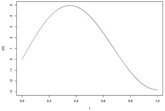
Figure 1. Simulation result of $\widehat{\gamma }(t)$ when $\rho =0.2,R=50,q=5,{\sigma }^2=0.25$. The solid curve denotes the true curve, the dash curve denotes its estimate.

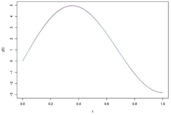
Figure 2. Simulation result of $\widehat{\gamma }(t)$ when $\rho =0.7,R=70,q=5,{\sigma }^2=1$. The solid curve denotes the true curve, the dash curve denotes its estimate.

From Table 1, Table 2 and Table 3 and Figure 1 and Figure 2 we can see that: (1) The biases of $\widehat{\rho }$, ${\widehat{\beta }}_1$ and ${\widehat{\beta }}_2$ are fairly small for almost all cases. (2) The standard deviation of $\widehat{\rho }$, ${\widehat{\beta }}_1$ and ${\widehat{\beta }}_2$ decrease as either R or q increases. (3) The RASEs of $\gamma (t)$ are small for all cases and decrease as sample size n increases or ${\sigma }^2$ decreases, and it can be concluded that the estimate curves fit better to the corresponding true line, which coincides with what was discovered from Figure 1 and Figure 2. Overall, the simulation results suggest that the proposed estimation procedure is effective for the partial functional linear spatial autoregressive model.

5. Conclusions

In this paper, we proposed a partial functional linear spatial autoregressive model to study the link between a scalar dependence spatial response variable and explanatory variables containing both multiple real-valued scalar variables and a functional predictor. We then used functional principal component basis and an instrumental variable to estimate the parametric vector and slope function based on the two-stage least squares procedure. Under some mild conditions, we obtained the asymptotic normality of estimators of a parametric vector. Furthermore, the rate of convergence of the proposed estimator of slope function was also established. The simulation studies demonstrate that the proposed method performs satisfactorily and the theoretical results are valid.

There are some interesting future directions. In this paper, we only considered the estimation of the unknown parametric vector and slope function, which does not present a way to test for the effects of the covariates, an important aspect of any statistical analysis. In the future, we would like to be able to identify the model structure by testing for the main effects of the scalar predictors and the functional predictor. Another interesting direction can be to extend our new procedure to the generalized partial functional linear spatial autoregressive model.

References

- Ramsay, J.O.; Silverman, B.W. Functional Data Analysis; Springer: New York, NY, USA, 1997. [Google Scholar]
- Cardot, H.; Ferraty, F.; Sarda, P. Spline estimators for the functional linear model. Statist. Sin. 2003, 13, 571–592. [Google Scholar]
- Yao, F.; Müller, H.G.; Wang, J.L. Functional linear regression analysis for longitudinal data. Ann. Statist. 2005, 33, 2873–2903. [Google Scholar] [CrossRef]
- Lian, H.; Li, G. Series expansion for functional sufficient dimension reduction. J. Multivariate Anal. 2014, 124, 150–165. [Google Scholar] [CrossRef]
- Fan, Y.; James, G.M.; Radchenko, P. Functional additive regression. Ann. Statist. 2015, 43, 2296–2325. [Google Scholar] [CrossRef]
- Feng, S.Y.; Xue, L.G. Partially functional linear varying coefficient model. Statistics 2016, 50, 717–732. [Google Scholar] [CrossRef]
- Kong, D.; Xue, K.; Yao, F.; Zhang, H.H. Partially functional linear regression in high dimensions. Biometrika 2016, 103, 147–159. [Google Scholar] [CrossRef]
- Yu, P.; Du, J.; Zhang, Z.Z. Varying-coefficient partially functional linear quantile regression models. J. Korean Statist. Soc. 2017, 46, 462–475. [Google Scholar] [CrossRef]
- Zhang, D.; Lin, X.; Sowers, M.F. Assessing the effects of reproductive hormone profiles on bone mineral density using functional two-stage mixed models. Biometrics 2007, 63, 351–362. [Google Scholar] [CrossRef] [PubMed]
- Shin, H. Partial functional linear regression. J. Statist. Plann. Inference 2009, 139, 3405–3418. [Google Scholar] [CrossRef]
- Lu, Y.; Du, J.; Sun, Z. Functional partially linear quantile regression model. Metrika 2014, 77, 317–332. [Google Scholar] [CrossRef]
- Yu, P.; Zhang, Z.Z.; Du, J. A test of linearity in partial functional linear regression. Metrika 2016, 79, 953–969. [Google Scholar] [CrossRef]
- Cliff, A.; Ord, J.K. Spatial Autocorrelation; Pion: London, UK, 1973. [Google Scholar]
- Anselin, L. Spatial Econometrics: Methods and Models; Kluwer: Dordrecht, The Netherlands, 1988. [Google Scholar]
- Cressie, N. Statistics for Spatial Data; John Wiley & Sons: New York, NY, USA, 1993. [Google Scholar]
- Lee, L.F. Asymptotic distributions of quasi-maximum likelihood estimators for spatial econometric models. Econometrica 2004, 72, 1899–1926. [Google Scholar] [CrossRef]
- Su, L.; Jin, S. Profile quasi-maximum likelihood estimation of partially linear spatial autoregressive models. J. Econom. 2010, 157, 18–33. [Google Scholar] [CrossRef]
- Koch, M.; Krisztin, T. Applications for asynchronous multi-agent teams in nonlinear applied spatial econometrics. J. Internet Technol. 2014, 12, 1007–1014. [Google Scholar]
- Chen, J.; Wang, R.; Huang, Y. Semiparametric spatial autoregressive model: A two-step bayesian approach. Ann. Public Health Res. 2015, 2, 1012–1024. [Google Scholar]
- Du, J.; Sun, X.Q.; Cao, R.Y.; Zhang, Z.Z. Statistical inference for partially linear additive spatial autoregressive models. Spat. Statist. 2018, 25, 52–67. [Google Scholar] [CrossRef]
- Dauxois, J.; Pousse, A.; Romain, Y. Asymptotic theory for the principal component analysis of a vector random function: Some applications to statistical inference. J. Multivariate Anal. 1982, 12, 136–154. [Google Scholar] [CrossRef]
- Cardot, H.; Ferraty, F.; Sarda, P. Functional linear model. Statist. Probab. Lett. 1999, 45, 11–22. [Google Scholar] [CrossRef]
- Hall, P.; Horowitz, J.L. Methodology and convergence rates for functional linear regression. Ann. Statist. 2007, 35, 70–91. [Google Scholar] [CrossRef]
- Hall, P.; Hosseini-nasab, M. Theory for high-order bounds in functional principal components analysis. Math. Proc. Cambridge Philos. Soc. 2009, 146, 225–256. [Google Scholar] [CrossRef]
- Kelejian, H.H.; Prucha, I.R. A generalized spatial two-stage least squares procedure for estimating a spatial autoregressive model with autoregressive disturbances. J. Real Estate Financ. 1998, 17, 99–121. [Google Scholar] [CrossRef]
- Zhang, Y.Q.; Shen, D.M. Estimation of semi-parametric varying-coefficient spatial panel data models with random-effects. J. Statist. Plann. Inference 2015, 159, 64–80. [Google Scholar] [CrossRef]
- Hu, Y.P.; Xue, L.G.; Zhao, J.; Zhang, L.Y. Skew-normal partial functional linear model and homogeneity test. J. Statist. Plann. Inference 2020, 204, 116–127. [Google Scholar] [CrossRef]
- Case, A.C. Spatial patterns in household demand. Econometrica 1991, 59, 953–965. [Google Scholar] [CrossRef]
© 2020 by the authors. Licensee MDPI, Basel, Switzerland. This article is an open access article distributed under the terms and conditions of the Creative Commons Attribution (CC BY) license (http://creativecommons.org/licenses/by/4.0/).