Article

Numerical Solutions of Fractional Differential Equations by Using Fractional Explicit Adams Method

by
Nur Amirah Zabidi
1,
Zanariah Abdul Majid
1,2,*,
Adem Kilicman
1,2 and
Faranak Rabiei
3
1
Institute for Mathematical Research, Universiti Putra Malaysia, UPM Serdang 43400, Malaysia
2
Department of Mathematics, Faculty of Science, Universiti Putra Malaysia, UPM Serdang 43400, Malaysia
3
School of Engineering, Monash University Malaysia, Jalan Lagoon Selatan, Bandar Sunway, Selangor 47500, Malaysia
*
Author to whom correspondence should be addressed.
Mathematics 2020, 8(10), 1675; https://doi.org/10.3390/math8101675
Submission received: 20 August 2020 / Revised: 18 September 2020 / Accepted: 19 September 2020 / Published: 1 October 2020
(This article belongs to the Special Issue Nonlinear Equations: Theory, Methods, and Applications)

Abstract

:
Differential equations of fractional order are believed to be more challenging to compute compared to the integer-order differential equations due to its arbitrary properties. This study proposes a multistep method to solve fractional differential equations. The method is derived based on the concept of a third-order Adam–Bashforth numerical scheme by implementing Lagrange interpolation for fractional case, where the fractional derivatives are defined in the Caputo sense. Furthermore, the study includes a discussion on stability and convergence analysis of the method. Several numerical examples are also provided in order to validate the reliability and efficiency of the proposed method. The examples in this study cover solving linear and nonlinear fractional differential equations for the case of both single order as α ( 0 , 1 ) and higher order, α 1 , 2 , where α denotes the order of fractional derivatives of D α y ( t ) . The comparison in terms of accuracy between the proposed method and other existing methods demonstrate that the proposed method gives competitive performance as the existing methods.

1. Introduction

Fractional calculus, particularly fractional differential equation (FDE), has significant applications, which thus plays a crucial role in various fields of science and engineering such as signal processing [1], control theory [2], modeling of materials [3] and diffusion processes [4]. The work by Woon [5] mentions the important implications of mathematical applications in other sciences such as physics. In addition, a study by Bagley and Torvik [6] remarks that fractional modelings are also extensively used in the field of viscoelasticity due to its ability to describe the high-frequency behavior of many viscoelastic materials.
First and foremost, we study the fractional initial value problem (FIVP) in the form [7],
C D t 0 α y ( t ) = f ( t , y ( t ) ) , y ( t 0 ) = y 0
where 0 < α < 1 is the fractional order and C D t 0 α denotes the fractional Caputo’s α - derivative operator C D t 0 α = R L D t 0 α ( y ( t ) y ( t 0 ) ) with R L D t 0 α ( y ( t ) ) is the Riemann–Liouville differential operator defined as [8]:
R L D t 0 α y ( t ) = 1 Γ ( m α ) d d t m t 0 t y ( τ ) d τ ( t τ ) α m + 1 , α > 0 , m = α .
The definition in Equation (2) has been applied especially in seeking for an analytical solution. However, when it comes to the real application, it might be very challenging. This is because, as pointed out by [9], specific additional conditions are needed to solve a differential equation in order to obtain a unique solution. These additional conditions for the Riemann–Liouville fractional derivative constitute a certain fractional derivative of unknown solution at the initial points which might result in an unclear physical meaning. Due to this reason, in the present work, we consider the fractional Caputo’s α -derivative, C D t 0 α (in sequel, we shall simply denote as D α ), which is defined as [10]
D α y ( t ) = 1 Γ ( m α ) t 0 t y ( m ) ( τ ) d τ ( t τ ) α m + 1 , m 1 < α < m Z + ,
where α > 0 and m = α ; see also [11].
In literature, several analytical and numerical methods have been developed over the past few decades, namely the variational iteration method [12,13], homotopy perturbation method [14,15] and the Adams–Bashforth–Moulton method [10] to solve the fractional differential and integral equations. However, in some cases, solving differential equations numerically has proven to be more efficient and convenient compared to analytical solutions especially when dealing with huge and complex problems. Therefore, many researchers have developed numerous numerical methods to solve various kinds of differential equations. For example, research by Podlunby [16] used the first order finite difference numerical method and managed to solve FDE problems with O ( h ) accuracy. Following that, Gorenflo [17] proposed a second order difference method to solve FDE and managed to achieve the desired accuracy. Another well-known numerical method of a predictor–corrector type has been developed by Diethelm et al. [18] In the study, they developed an algorithm of P ( E C ) m E (Predict–Evaluate–Correct–Evaluate) where m is the number of iterations to solve linear and nonlinear FDE. In addition, Galeone and Garrappa [19] present a study on multistep methods for differential equations of fractional order that concerns numerical treatment of FDE on both implicit and explicit types. They managed to prove that explicit methods in the treatment of FDE give a good numerical solution with good stability analysis. Later, Blaszczyk and Leszczynski [20] proposed a study on FDE of higher order with a mixture of integer and Caputo derivatives using Euler’s method. They modified the discrete form of the Caputo derivative being dependent on a range of the parameter, α and found that, when the range increases, the number of discrete equations occurring in the algorithm also increases.
The focus of this study is to derive an explicit multistep method based on the concept of the third-order Adams–Bashforth method, where the derivation of the proposed method is given in Section 2. Furthermore, the analysis of the stability and convergence is demonstrated in Section 3. Following from there, the implementation of the proposed method is shown in Section 4. The numerical results for solving six examples of FDEs are presented in Section 5, where it also includes a discussion on the numerical results obtained to illustrate the efficiency and effectiveness of the proposed method.

2. Fractional Explicit Adams Method of Order 3

This section will introduce a derivation of the fractional explicit Adams method of order 3 (FEAM3).
In the first step, consider the FIVP is in the form [21]:
D α y ( t ) = f ( t , y ( t ) ) , y k ( 0 ) = y 0 k , k = 0 , 1 , , α 1 .
It is well-known that FIVP in Equation (4) can be rewritten in the form equivalent to the Volterra integral equation [21] as:
y ( t ) = k = 0 α 1 t k k ! y k ( 0 ) + 1 Γ ( α ) 0 t [ ( t τ ) α 1 f ( τ , y ( τ ) ) ] d τ .
Note that, according to Diethelm [22], it is common to consruct methods for FDE by taking methods for classical (typically first-order) equations and generalizing the concept in an appropriate way. Therefore, we have Equation (4) as:
D y ( t ) = f ( t , y ( t ) ) , y ( 0 ) = y 0 .
Next, simplify Equation (5) as [23]:
y ( t ) = y 0 + 1 Γ ( α ) 0 t [ ( t τ ) α 1 f ( τ , y ( τ ) ) ] d τ .
Now, we propose an approximate solution that involves approximation at the points t = t n and t = t n + 1 . Thus,
i.
If t = t n ;
y ( t n ) = y 0 + 1 Γ ( α ) 0 t n [ ( t n τ ) α 1 f ( τ , y ( τ ) ) ] d τ
ii.
If t = t n + 1 ;
y ( t n + 1 ) = y 0 + 1 Γ ( α ) 0 t n + 1 [ ( t n + 1 τ ) α 1 f ( τ , y ( τ ) ) ] d τ .
Subtracting Equation (9) from Equation (8) will yield:
y ( t n + 1 ) = y ( t n ) + 1 Γ ( α ) 0 t n + 1 ( t n + 1 τ ) α 1 f ( τ , y ( τ ) ) d τ 0 t n ( t n τ ) α 1 f ( τ , y ( τ ) ) d τ .
The proposed method is of order 3; therefore, taking the Lagrange interpolation with three interpolating functions of F n , F n 1 and F n 2 are required to evaluate the approximate solutions as follows:
P ( t ) ( f ( τ , y ( τ ) ) ) = ( t t n 1 ) ( t t n 2 ) ( t n t n 1 ) ( t n t n 2 ) F n + ( t t n ) ( t t n 2 ) ( t n 1 t n ) ( t n 1 t n 2 ) F n 1 + ( t t n ) ( t t n 1 ) ( t n 2 t n ) ( t n 2 t n 1 ) F n 2
Next, let:
h = t n + 1 t n , τ = t .
Substituting Equations (11) and (12) into Equation (10), we obtain:
y ( t n + 1 ) = y ( t n ) + 1 Γ ( α ) 0 t n + 1 ( t n + 1 t ) α 1 ( t t n 1 ) ( t t n 2 ) ( t n t n 1 ) ( t n t n 2 ) F n + ( t t n ) ( t t n 2 ) ( t n 1 t n ) ( t n 1 t n 2 ) F n 1 + ( t t n ) ( t t n 1 ) ( t n 2 t n ) ( t n 2 t n 1 ) F n 2 d t 1 Γ ( α ) 0 t n ( t n t ) α 1 ( t t n 1 ) ( t t n 2 ) ( t n t n 1 ) ( t n t n 2 ) F n + ( t t n ) ( t t n 2 ) ( t n 1 t n ) ( t n 1 t n 2 ) F n 1 + ( t t n ) ( t t n 1 ) ( t n 2 t n ) ( t n 2 t n 1 ) F n 2 d t .
i.
The first fractional integral is evaluated as:
0 t n + 1 ( t n + 1 t ) α 1 f ( τ , y ( τ ) ) d τ = p = 0 n t p t p + 1 ( t n + 1 t ) α 1 ( t t n 1 ) ( t t n 2 ) ( t n t n 1 ) ( t n t n 2 ) F n + ( t t n ) ( t t n 2 ) ( t n 1 t n ) ( t n 1 t n 2 ) F n 1 + ( t t n ) ( t t n 1 ) ( t n 2 t n ) ( t n 2 t n 1 ) F n 2 d t = p = 0 n F n ( t n t n 1 ) ( t n t n 2 ) t p t p + 1 ( t n + 1 t ) α 1 ( t t n 1 ) ( t t n 2 ) d t + F n 1 ( t n 1 t n ) ( t n 1 t n 2 ) t p t p + 1 ( t n + 1 t ) α 1 ( t t n ) ( t t n 2 ) d t + F n 2 ( t n 2 t n ) ( t n 2 t n 1 ) t p t p + 1 ( t n + 1 t ) α 1 ( t t n ) ( t t n 1 ) d t = p = 0 n F n 2 h 2 t p t p + 1 ( t n + 1 t ) α 1 ( t t n 1 ) ( t t n 2 ) d t F n 1 h 2 t p t p + 1 ( t n + 1 t ) α 1 ( t t n ) ( t t n 2 ) d t + F n 2 2 h 2 t p t p + 1 ( t n + 1 t ) α 1 ( t t n ) ( t t n 1 ) d t .
Now, consider making substitution y = t n + 1 t , d y = d t ; then:
p = 0 n F n 2 h 2 t n + 1 t p t n + 1 t p + 1 ( y ) α 1 ( t n + 1 y t n 1 ) ( t n + 1 y t n 2 ) d y F n 1 h 2 t n + 1 t p t n + 1 t p + 1 ( y ) α 1 ( t n + 1 y t n ) ( t n + 1 y t n 2 ) d y + F n 2 2 h 2 t n + 1 t p t n + 1 t p + 1 ( y ) α 1 ( t n + 1 y t n ) ( t n + 1 y t n 1 ) d y = F n 2 h 2 6 h 2 α [ ( t n + 1 t n + 1 ) α ( t n + 1 t 0 ) α ] + 5 h α + 1 [ ( t n + 1 t n + 1 ) α + 1 ( t n + 1 t 0 ) α + 1 ] 1 α + 2 [ ( t n + 1 t n + 1 ) α + 2 ( t n + 1 t 0 ) α + 2 ] F n 1 h 2 3 h 2 α [ ( t n + 1 t n + 1 ) α ( t n + 1 t 0 ) α ] + 4 h α + 1 [ ( t n + 1 t n + 1 ) α + 1 ( t n + 1 t 0 ) α + 1 ] 1 α + 2 [ ( t n + 1 t n + 1 ) α + 2 ( t n + 1 t 0 ) α + 2 ] + F n 2 2 h 2 2 h 2 α [ ( t n + 1 t n + 1 ) α ( t n + 1 t 0 ) α ] + 3 h α + 1 [ ( t n + 1 t n + 1 ) α + 1 ( t n + 1 t 0 ) α + 1 ] 1 α + 2 [ ( t n + 1 t n + 1 ) α + 2 ( t n + 1 t 0 ) α + 2 ] .
Thus, the computation for the first fractional integral is given by:
h α 3 ( n + 1 ) α α 5 ( n + 1 ) α + 1 2 α + 2 + ( n + 1 ) α + 2 2 α + 4 F n 3 ( n + 1 ) α α 4 ( n + 1 ) α + 1 α + 1 + ( n + 1 ) α + 2 α + 2 F n 1 + ( n + 1 ) α α 3 ( n + 1 ) α + 1 2 α + 2 + ( n + 1 ) α + 2 2 α + 4 F n 2 .
ii.
Similar to the above steps, the second fractional integral can be computed as in the following form:
0 t n ( t n t ) α 1 f ( τ , y ( τ ) ) d τ = p = 0 n 1 t p t p + 1 ( t n t ) α 1 ( t t n 1 ) ( t t n 2 ) ( t n t n 1 ) ( t n t n 2 ) F n + ( t t n ) ( t t n 2 ) ( t n 1 t n ) ( t n 1 t n 2 ) F n 1 + ( t t n ) ( t t n 1 ) ( t n 2 t n ) ( t n 2 t n 1 ) F n 2 d t = p = 0 n 1 F n 2 h 2 t p t p + 1 ( t n t ) α 1 ( t t n 1 ) ( t t n 2 ) d t F n 1 h 2 t p t p + 1 ( t n t ) α 1 ( t t n ) ( t t n 2 ) d t + F n 2 2 h 2 t p t p + 1 ( t n t ) α 1 ( t t n ) ( t t n 1 ) d t .
Next, making the changes y = t n t and d y = d t gives:
p = 0 n 1 F n 2 h 2 t n t p t n t p + 1 ( y ) α 1 ( t n y t n 1 ) ( t n y t n 2 ) d y F n 1 h 2 t n t p t n t p + 1 ( y ) α 1 ( t n y t n ) ( t n y t n 2 ) d y + F n 2 2 h 2 t n t p t n t p + 1 ( y ) α 1 ( t n y t n ) ( t n y t n 1 ) d y = F n 2 h 2 2 h 2 α [ ( t n t n ) α ( t n t 0 ) α ] + 3 h α + 1 [ ( t n t n ) α + 1 ( t n t 0 ) α + 1 ] 1 α + 2 [ ( t n t n ) α + 2 ( t n t 0 ) α + 2 ] F n 1 h 2 2 h α + 1 [ ( t n t n ) α + 1 ( t n t 0 ) α + 1 ] 1 α + 2 [ ( t n t n ) α + 2 ( t n t 0 ) α + 2 ] + F n 2 2 h 2 h α + 1 [ ( t n t n ) α + 1 ( t n t 0 ) α + 1 ] 1 α + 2 [ ( t n t n ) α + 2 ( t n t 0 ) α + 2 ] .
Therefore, we obtain the computation for the second fractional integral
h α ( n ) α α 3 ( n ) α + 1 2 α + 2 + ( n ) α + 2 2 α + 4 F n 2 ( n ) α + 1 α + 1 + ( n ) α + 2 α + 2 F n 1 + ( n ) α + 1 2 α + 2 + ( n ) α + 2 2 α + 4 F n 2 .
Now, if we substitute Equations (16) and (19) into Equation (10), then we obtain a numerical scheme for FEAM3 as follows:
y ( t n + 1 ) = y ( t n ) + h α Γ ( α ) 3 ( n + 1 ) α ( n ) α α + 3 ( n ) α + 1 5 ( n + 1 ) α + 1 2 α + 2 + ( n + 1 ) α + 2 ( n ) α + 2 2 α + 4 F n + 3 ( n + 1 ) α α + 4 ( n + 1 ) α + 1 2 ( n ) α + 1 α + 1 + ( n ) α + 2 ( n + 1 ) α + 2 α + 2 F n 1 + ( n + 1 ) α α + ( n ) α + 1 3 ( n + 1 ) α + 1 2 α + 2 + ( n + 1 ) α + 2 ( n ) α + 2 2 α + 4 F n 2 .
Therefore, Equation (20) is the proposed numerical scheme known as FEAM3. The method analysis and performance evaluation of FEAM3 are discussed in the latter section.

3. Analysis of the Method

3.1. Order of the Method

Definition 1
([24]). Linear multistep method is said to be of order p if, C 0 = C 1 = = C p = 0 and C p + 1 0 . The formula used to calculate the constant C p is given by:
C p = j = 0 k j p α j p ! j p 1 β j ( p 1 ) ! , p = 0 , 1 , 2 ,
where k is the order of the proposed method, α and β is the coefficient obtained from the proposed method. Note that C p + 1 is the error constant of the method.
In order to check the order of the method Equation (20), we consider the general formulation of fractional linear multistep method for the solution of Equation (4) [19] as:
j = 0 n α j y n j = h α j = 0 n β j f ( t n j , y n j )
where α j and β j are real parameters and α denotes the fractional order.
By comparing Equations (20) and (22), we obtain α j and β j as follows:
α 0 = 0 , β 0 = 1 Γ ( α ) ( n + 1 ) α α + ( n ) α + 1 3 ( n + 1 ) α + 1 2 α + 2 + ( n + 1 ) α + 2 ( n ) α + 2 2 α + 4 , α 1 = 0 , β 1 = 1 Γ ( α ) 3 ( n + 1 ) α α + 4 ( n + 1 ) α + 1 2 ( n ) α + 1 α + 1 + ( n ) α + 2 ( n + 1 ) α + 2 α + 2 , α 2 = 1 , β 2 = 1 Γ ( α ) 3 ( n + 1 ) α ( n ) α α + 3 ( n ) α + 1 5 ( n + 1 ) α + 1 2 α + 2 + ( n + 1 ) α + 2 ( n ) α + 2 2 α + 4 , α 3 = 1 , β 3 = 0 .
Substitute Equation (23) into Equation (21) and it gives:
C 0 = j = 0 k α j = 0 . C 1 = j = 0 k ( j α j β j ) = 0 . C 2 = j = 0 k ( j 2 α j 2 ! j β j ) = 0 . C 3 = j = 0 k ( j 3 α j 3 ! j 2 β j 2 ! ) = 0 . C 4 = j = 0 k ( j 4 α j 4 ! j 3 β j 3 ! ) = 3 8 .
Therefore, the method is proven to be of order 3 with error constant C 4 = 3 8 .

3.2. Stability Analysis

The following test equation [7] was considered in order to analyze the stability properties of FEAM3:
D α y ( t ) = λ y ( t ) , λ ϵ C , 0 < α < 1 , y ( t 0 ) = y 0
where the exact solution can be expressed in terms of the Mittag–Leffler function:
E α ( t ) = k = 0 t k Γ ( α k + 1 )
as y ( t ) = E α ( λ ( t t 0 ) α ) y 0 .
Substitute test Equation (25) into the numerical method in Equation (20), which resulted in the stability polynomial of:
y ( t n + 1 ) = y ( t n ) + h ¯ Γ ( α ) 3 ( n + 1 ) α ( n ) α α + 3 ( n ) α + 1 5 ( n + 1 ) α + 1 2 α + 2 + ( n + 1 ) α + 2 ( n ) α + 2 2 α + 4 y n + 3 ( n + 1 ) α α + 4 ( n + 1 ) α + 1 2 ( n ) α + 1 α + 1 + ( n ) α + 2 ( n + 1 ) α + 2 α + 2 y n 1 + ( n + 1 ) α α + ( n ) α + 1 3 ( n + 1 ) α + 1 2 α + 2 + ( n + 1 ) α + 2 ( n ) α + 2 2 α + 4 y n 2
where h ¯ = λ h α .
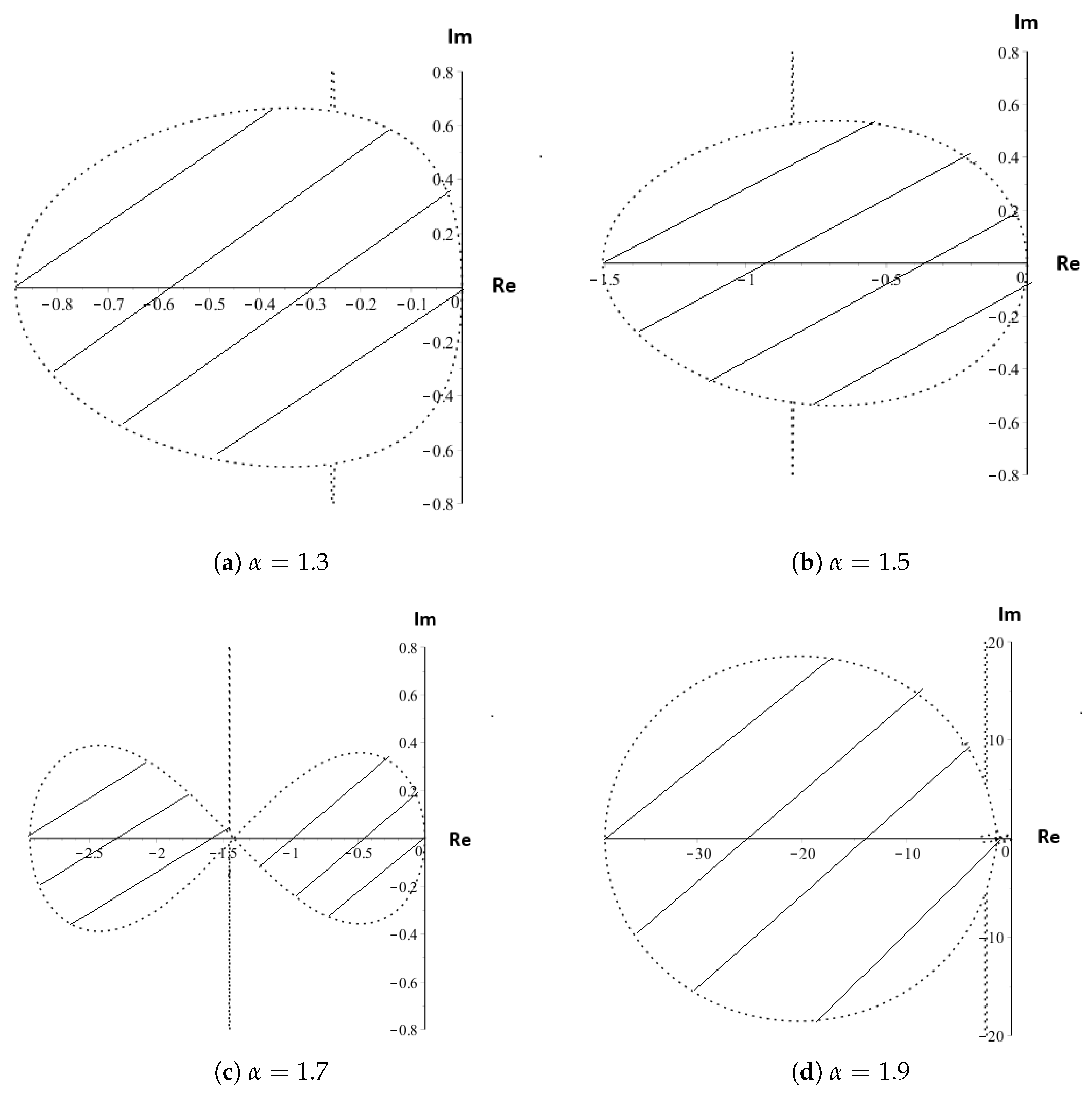
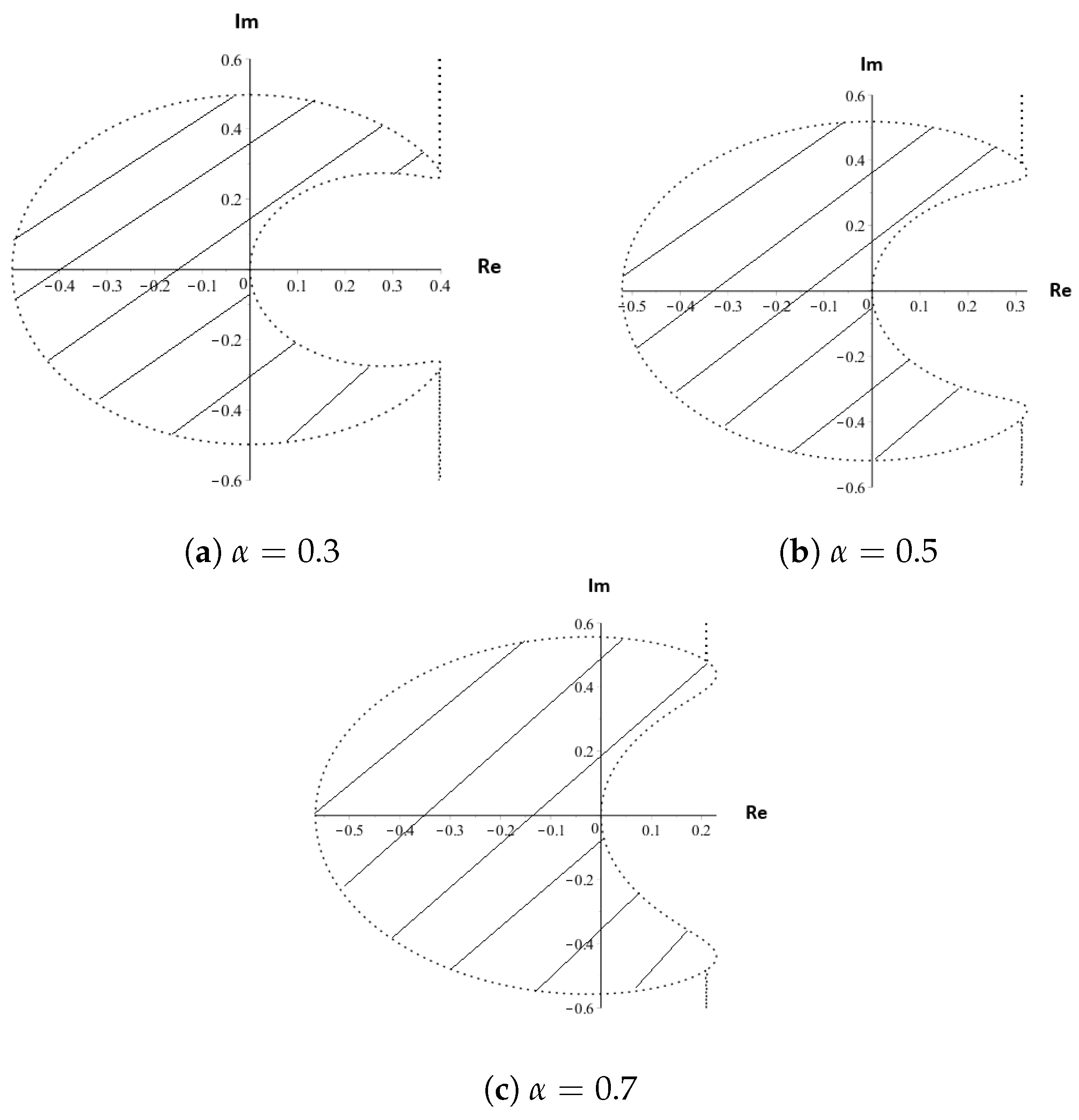
Next, taking Equation (26) into consideration, the stability region of FEAM3 is drawn as shown in Figure 1, Figure 2 and Figure 3 by using Maple software for different values of α . The planes are separated between the imaginary and the real field (horizontal axis, labelled as Re, represents Real while vertical axis, labelled as Im, represents Imaginary).

3.2.1. Single Order

A fractional equation is called single order FDE when 0 < α < 1 . For comparison purposes, this paper separates the analysis for both single and higher order FDE.
While investigating the stability analysis, we are interested to investigate the values of h ¯ = λ h α . To determine the stability region, we take into consideration whether every root of λ i is real and must satisfy | λ i | 1 as stated in [25]. Thus, as the result, Equation (26) proved to be stable inside the shaded region as shown in Figure 1. In addition, we can also see from Figure 1 and Figure 2 that, as the value of α increases, the stability region approaches to the left and is symmetric to the real axis. As for the area of the stability regions, we can observe from Figure 2 that the region became larger as the α increased.

3.2.2. Higher Order

In order to be considered as higher order FDE, the value of α should be when 1 < α < 2 . A similar strategy was applied to determine the stability region for higher order FDE where we were interested in investigating the values of h ¯ = λ h α of Equation (26).
As mentioned before, we take into consideration whether every root of λ i is real and must satisfy | λ i | 1 . Therefore, Equation (26) proved to be stable inside the shaded region as shown in Figure 3 when 1 < α < 2 . According to Figure 3, it shows that the region for higher order FDE also became larger as the α increased and approached 2. The regions are shown to become larger in the left imaginary axis and symmetric to the real axis.

3.3. Convergence Analysis

Recalling the proposed method, FEAM3 as in Equation (20), we have:
y ( t n + 1 ) = y ( t n ) + h α Γ ( α ) 3 ( n + 1 ) α ( n ) α α + 3 ( n ) α + 1 5 ( n + 1 ) α + 1 2 α + 2 + ( n + 1 ) α + 2 ( n ) α + 2 2 α + 4 F n + 3 ( n + 1 ) α α + 4 ( n + 1 ) α + 1 2 ( n ) α + 1 α + 1 + ( n ) α + 2 ( n + 1 ) α + 2 α + 2 F n 1 + ( n + 1 ) α α + ( n ) α + 1 3 ( n + 1 ) α + 1 2 α + 2 + ( n + 1 ) α + 2 ( n ) α + 2 2 α + 4 F n 2 .
Then, we have the following theorems to prove the convergence properties of FEAM3.
Let:
A = 3 ( n + 1 ) α ( n ) α α + 3 ( n ) α + 1 5 ( n + 1 ) α + 1 2 α + 2 + ( n + 1 ) α + 2 ( n ) α + 2 2 α + 4 B = 3 ( n + 1 ) α α + 4 ( n + 1 ) α + 1 2 ( n ) α + 1 α + 1 + ( n ) α + 2 ( n + 1 ) α + 2 α + 2 C = ( n + 1 ) α α + ( n ) α + 1 3 ( n + 1 ) α + 1 2 α + 2 + ( n + 1 ) α + 2 ( n ) α + 2 2 α + 4
Next, by implementing Equation (27) into Equation (20), we have:
i
The exact form of the system is given by:
y * ( t n + 1 ) y * ( t n ) = h α Γ ( α ) A F n * + h α Γ ( α ) B F n 1 * + h α Γ ( α ) C F n 2 * + 3 8 h 4 Y 4 ( ξ )
ii
The approximate form of the system is:
y ( t n + 1 ) y ( t n ) = h α Γ ( α ) A F n + h α Γ ( α ) B F n 1 + h α Γ ( α ) C F n 2
Now, subtracting Equation (29) from Equation (28) will give:
y ( t n + 1 ) y * ( t n + 1 ) = y ( t n ) y * ( t n ) + h α Γ ( α ) ( A ) [ f ( t n , y n ) f ( t n * , y n * ) ] + h α Γ ( α ) ( B ) [ f ( t n 1 , y n 1 ) f ( t n 1 * , y n 1 * ) ] + h α Γ ( α ) ( C ) [ f ( t n 2 , y n 2 ) f ( t n 2 * , y n 2 * ) ] + 3 8 h 4 Y 4 ( ξ ) .
Let:
| d n + 1 | = | y n + 1 y n + 1 * | , | d n | = | y n y n * | , | d n 1 | = | y n 1 y n 1 * | , | d n 2 | = | y n 2 y n 2 * | .
Next, applying Lipschitz condition as in Theorem 1 and the assumption in Equation (31), we have:
d n + 1 1 + h α A Γ ( α ) d n + h α B Γ ( α ) d n 1 + h α C Γ ( α ) d n 2 + 3 8 h 4 β .
Rewriting Equation (32) based on Theorem 2, we obtain:
d n + 1 1 + K h α d n + K h α d n 1 + K h α d n 2 + 3 8 h 4 β .
From the above analysis, it can be seen that, as h 0 , it is proven that | d n + 1 | | d n | ; thus,  | y n + 1 | = | y n + 1 * | and | y n | = | y n * | . In conclusion, Theorem 2 is satisfied. Hence, the proposed method, FEAM3, is proved to converge.
Theorem 1
([22]). Let f ( t , y ) be Lipschitz continuous at all points ( t , y ) in a region D, given by:
a t b , < y < ,
such that, for every t , y , y * , the coordinates t , y , y * and ( t , y * ) are both in D where
D α y ( t ) = f ( t , y ( t ) ) .
Theorem 2
([10,22,26]). A linear multistep method is said to be convergent if, for all initial value problems subject to the hypothesis of Theorem 1 as t [ a , b ] , we have that:
y y * K t α 1 h p ,
where K is a constant that depends only on α and p as p ( 0 , 1 ) , 0 < α < 1 and
lim h 0 y n = y ( t n ) .

4. Implementation

Algorithm of the Method

This section includes the algorithm of the proposed method. The inputs of the programming are the values of endpoints, a and b, number of intervals, N, the value of α as well as the initial value, y 0  as 0 < α < 1 and y 0 , y 0 as 1 < α < 2 . The developed algorithm for the method is illustrated in Algorithm 1.
Algorithm 1 The FEAM3 method.
1:
Step 1. Set t o l = 10 7 , t 0 = a , t 1 = b , y 0 = c , y 0 = d , α = a l p h a , Γ ( α ) = g a m m a and h = b a N .
2:
Step 2. For n = 0 , 1 , calculate the approximation solution, y 1 , y 2 using Fractional Euler method [27]:
3:
          y ( t n + 1 ) = y ( t n ) + h α Γ ( α + 1 ) ( F n ) .
4:
Step 3. For n = 2 , 3 , , N , calculate the approximation solution, y 3 , y 4 , , y N
5:
         by iterating the procedure in steps 4–7.
6:
Step 4. Set t = a + n h and s u m = 0 .
7:
Step 5. Evaluate for y n + 1 by using the FEAM3 as in Equation (20).
8:
Step 6. Next, check the maximum error.
9:
         Note that, error = y n Y n , where y n is the approximation solution and Y n is the exact
10:
         solution.
11:
        If error > tolerance,
12:
        OUTPUT: error= maximum error.
13:
Step 7. Calculate the average error using:
14:
         average error = ( s u m + e r r o r ) / N ,
15:
         s u m = average error,
16:
        OUTPUT: average error.
17:
Step 8. The procedure is completed.

5. Numerical Results

In order to validate the efficiency of the proposed method, six tested FDE problems which consist of single order as 0 < α < 1 and higher order, 1 α < 2 were considered. The computation was done using C programming (CodeBlock). Below are the notations used in the tables:
NNumber of intervals.
hStep size.
Approx.Approximate solution.
ErrorAbsolute error.
FEAM3Fractional Explicit Adams Method order 3 (in this research).
FAMFractional Adams Method [21].
FLMM-3Fractional Linear Multistep Method of Order 3 [25].
ATPCAdams-Type Predictor Corrector Method [18].
SFMoPFSpline Function Method of Polynomial Form [28].
3-HOFLMSMHigh Order Fractional Linear Multistep Method of 3-order [29].
FVIMFractional Variational Iteration method [30].
MHPMModified Homotophy Pertubation method [31].
Example 1.
A simple linear fractional differential equations [21], given
D α y ( t ) = y ( t ) , y ( 0 ) = 1 , y ( 0 ) = 0 .
The exact solution is y ( t ) = E α ( t α ) , where E α ( z ) is the Mittag–Leffler function defined as
E α ( z ) = k = 0 z k Γ ( α k + 1 ) .
Example 2.
An initial value problem of FDE [25].
D α y ( t ) = Γ ( 2 α + 1 ) Γ ( α + 1 ) t α 2 Γ ( 3 α ) t 2 α + t 2 α t 2 4 y 4 ( t ) , y ( 0 ) = 0
where the exact solution is given by y ( t ) = t 2 α t 2 .
Example 3.
A problem of FIVP with variable coefficients [18] is given by
D α y ( t ) = 40320 Γ ( 9 α ) t 8 α 3 Γ ( 5 + α / 2 ) Γ ( 5 α / 2 ) t 4 α / 2 + 9 4 Γ ( α + 1 ) + 3 2 t α / 2 t 4 3 [ y ( t ) ] 3 / 2 , y ( 0 ) = 0 , y ( 0 ) = 0 .
The exact solution is y ( t ) = t 8 3 t 4 + α / 2 + 9 4 t α .
Example 4.
A nonlinear initial value problem of FDE [28] is given by
D α y ( t ) = 1 y ( t ) 4 , y ( 0 ) = 0 .
The exact solution is y ( t ) = 1 + 3 t ( 1 + 6 t + 9 t 2 ) 1 3 ( 1 + 3 t ) as α = 1.0 .
Example 5.
A problem of higher order nonlinear fractional differential equation [29].
D α y ( t ) + y 2 ( t ) = f ( t ) , y ( 0 ) = 0 , y ( 0 ) = 0 ,
where
f ( t ) = Γ ( 6 ) Γ ( 6 α ) t 5 α 3 Γ ( 5 ) Γ ( 5 α ) t 4 α + 2 Γ ( 4 ) Γ ( 4 α ) t 3 α + t 5 3 t 4 + 2 t 3 2 .
The results are tabulated when α = 1.50 where the exact solution is y ( t ) = t 5 3 t 4 + 2 t 3 .
Example 6.
An application problem of fractional Riccati differential equations [30,31].
D α y ( t ) = y 2 ( t ) + 1 , y ( 0 ) = 0 .
The exact solution is y ( t ) = e 2 t 1 e 2 t + 1 when α = 1.0 .
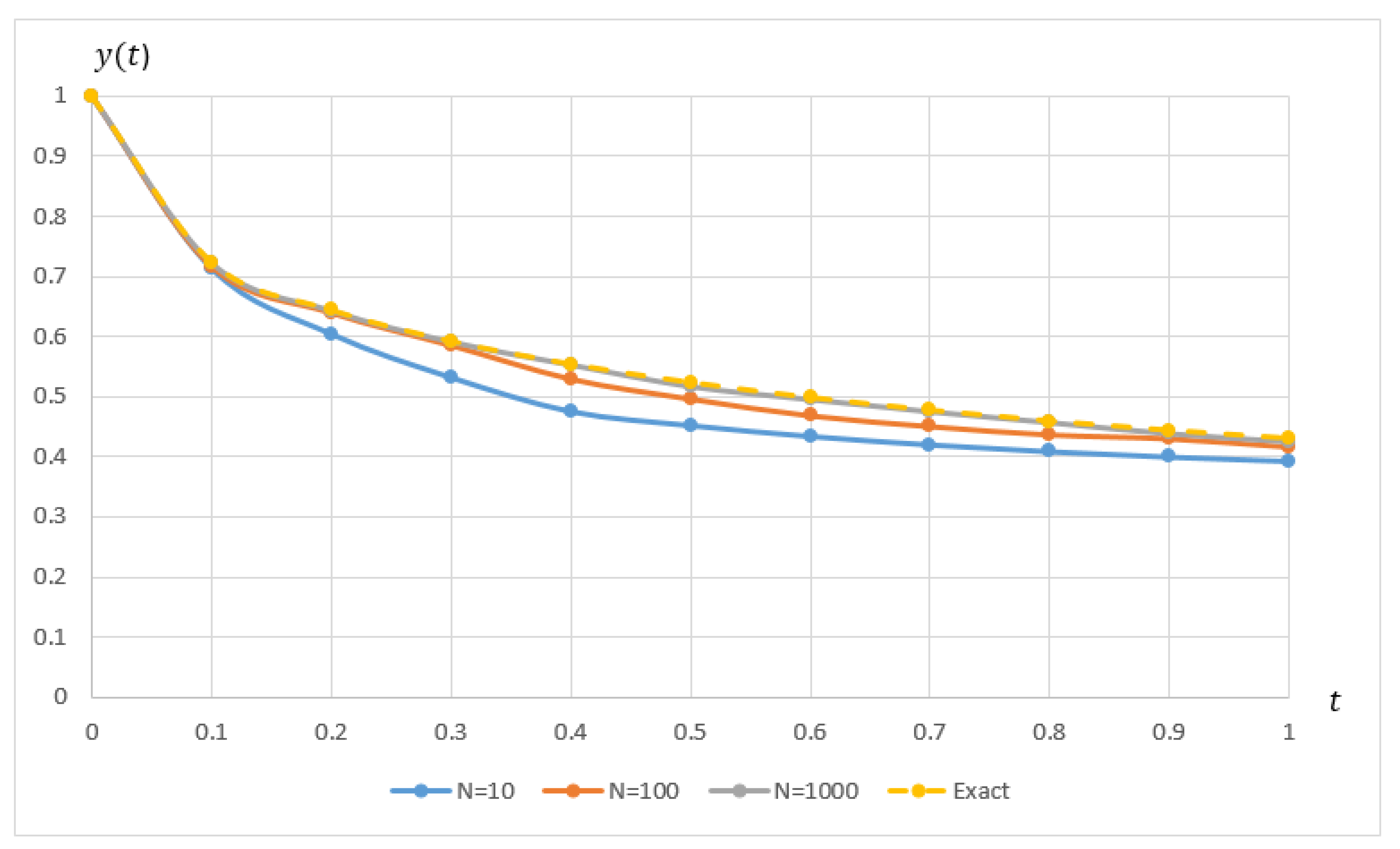
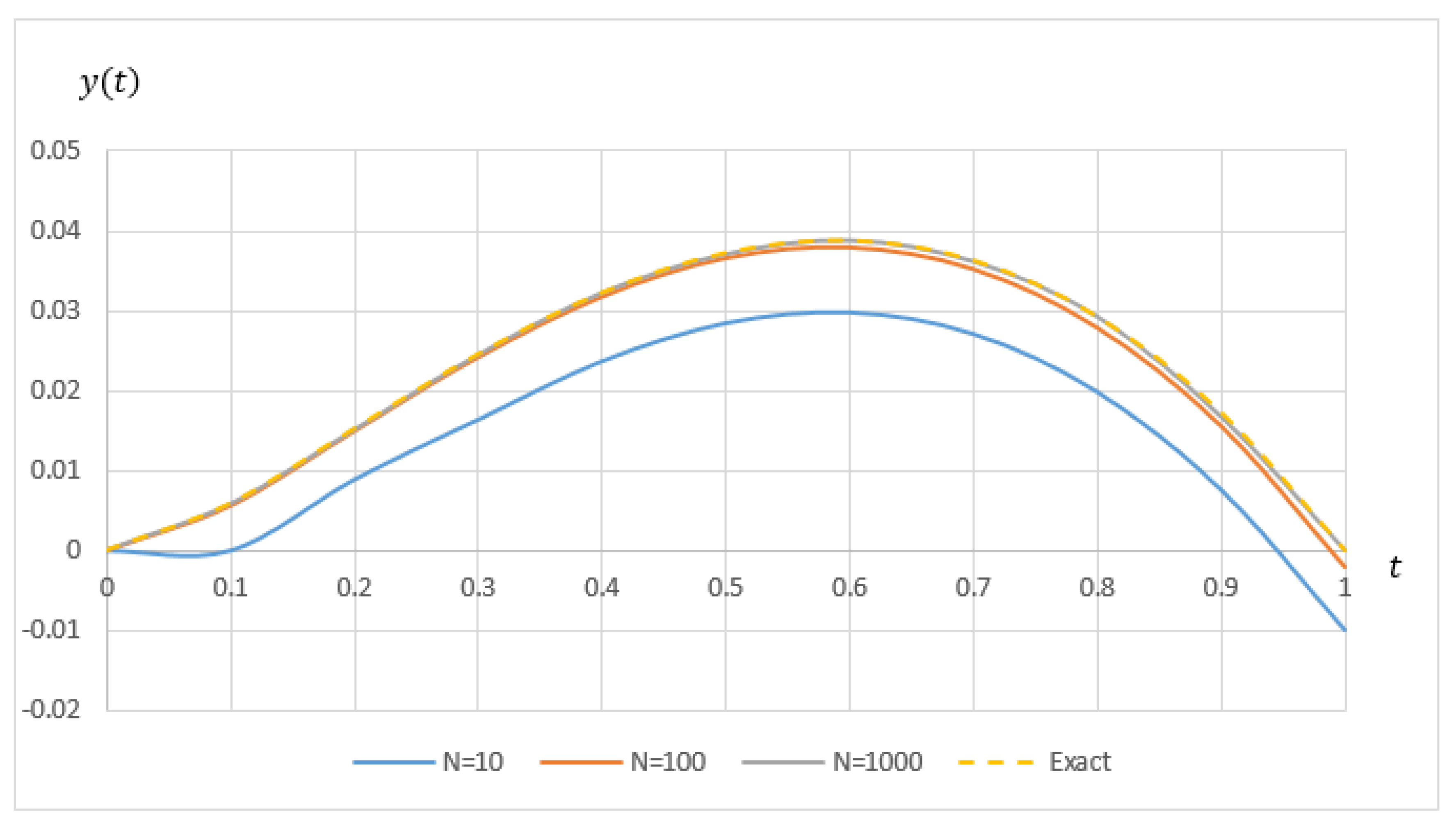
Table 1 and Table 2 demonstrate the absolute error for solving a simple linear FDE of variable coefficient where the exact solution is the Mittag–Leffler function. Table 1 shows the absolute error of single order FDE as α = 0.30 , 0.50 , 0.70 , while Table 2 presents the absolute error of higher order FDE as α = 1.30 , 1.70 , 1.90 at different step size, h = 10 3 , 10 4 . Based on these tables, it can be seen that, for each step size, h, the absolute error decreases as the order of FDE, and α increases. In addition, Table 3 shows the comparison in terms of absolute error at point, t = 1.0 when solving Example 1 between FAM and FEAM3 as α = 0.10 , 0.90 , 1.25 , 1.85 at N = 10 , 20 , 40 , 80 , 160 , 320 . From the table, it can be seen that FEAM3 managed to produce comparable results as FAM. The performance graph for solving single and higher order of Example 1 are shown in Figure 4 and Figure 5 respectively. The graphs illustrate that, for both cases, the approximate solution clearly approaches the exact solution when N increases.
Table 4 displays the absolute error at each point, t for solving an initial value problem of FDE in single order as α = 0.30 , 0.50 , 0.70 at different step size, h = 10 3 , 10 4 . The table shows that FEAM3 managed to perform well, whereby, as h decreases and α approaches 1.0 , better accuracy was obtained. In order to observe the efficiency of FEAM3, Table 5, which displays the absolute error at point, t = 1 when solving Example 2 between FEAM3 and FLMM-3 when α = 0.7 , 0.8 at h = 0.1 , 0.01 , 0.001 is also included. Based on the table, it shows that a comparable result is obtained between FEAM3 and FLMM-3. For better analysis, the performance graph for Example 2 is included in Figure 6 for α = 0.50 at N = 10 , 100 , 1000 . Based on the graph, it can be seen that, as α increases, the approximate solutions approach the exact solution.
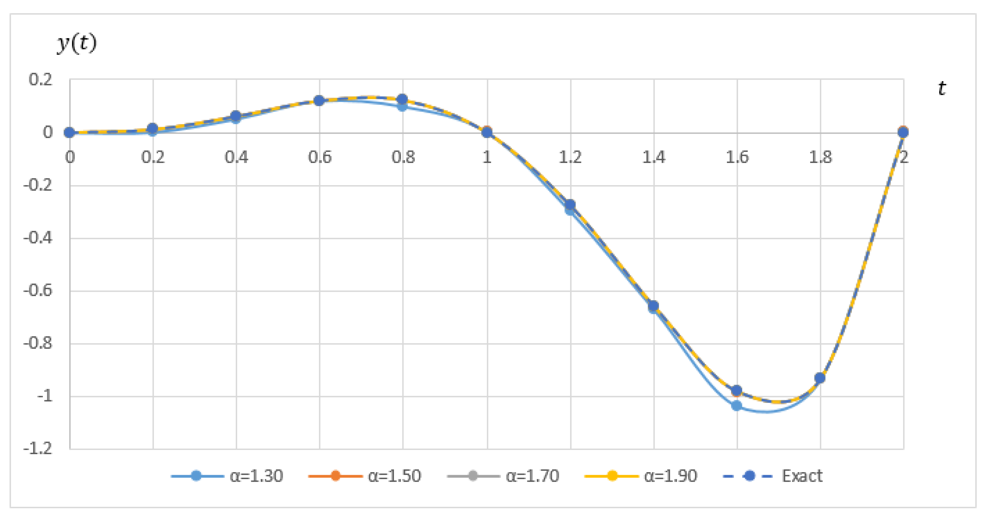
In addition, the numerical results for solving initial value problem of higher order FDE are tabulated in Table 6 in the form of absolute error when α = 1.30 , 1.70 , 1.90 as h = 10 3 , 10 4 . The table proved that FEAM3 is also able to perform well in solving nonlinear FDE, where the absolute error decreases when α increases and h decreases. On the other hand, Table 7 shows the absolute error of various α = 1.25 at different h between FEAM3 and ATPC for solving nonlinear FDE of Example 3, where FEAM3 is able to obtain a comparable result as the existing method, ATPC. Additionally, the graph of approximate solution at each point, t, for solving Example 3 when α = 1.50 for different N is shown in Figure 7. The graph highlights that the approximate solution does indeed approach the exact solution as α increases.
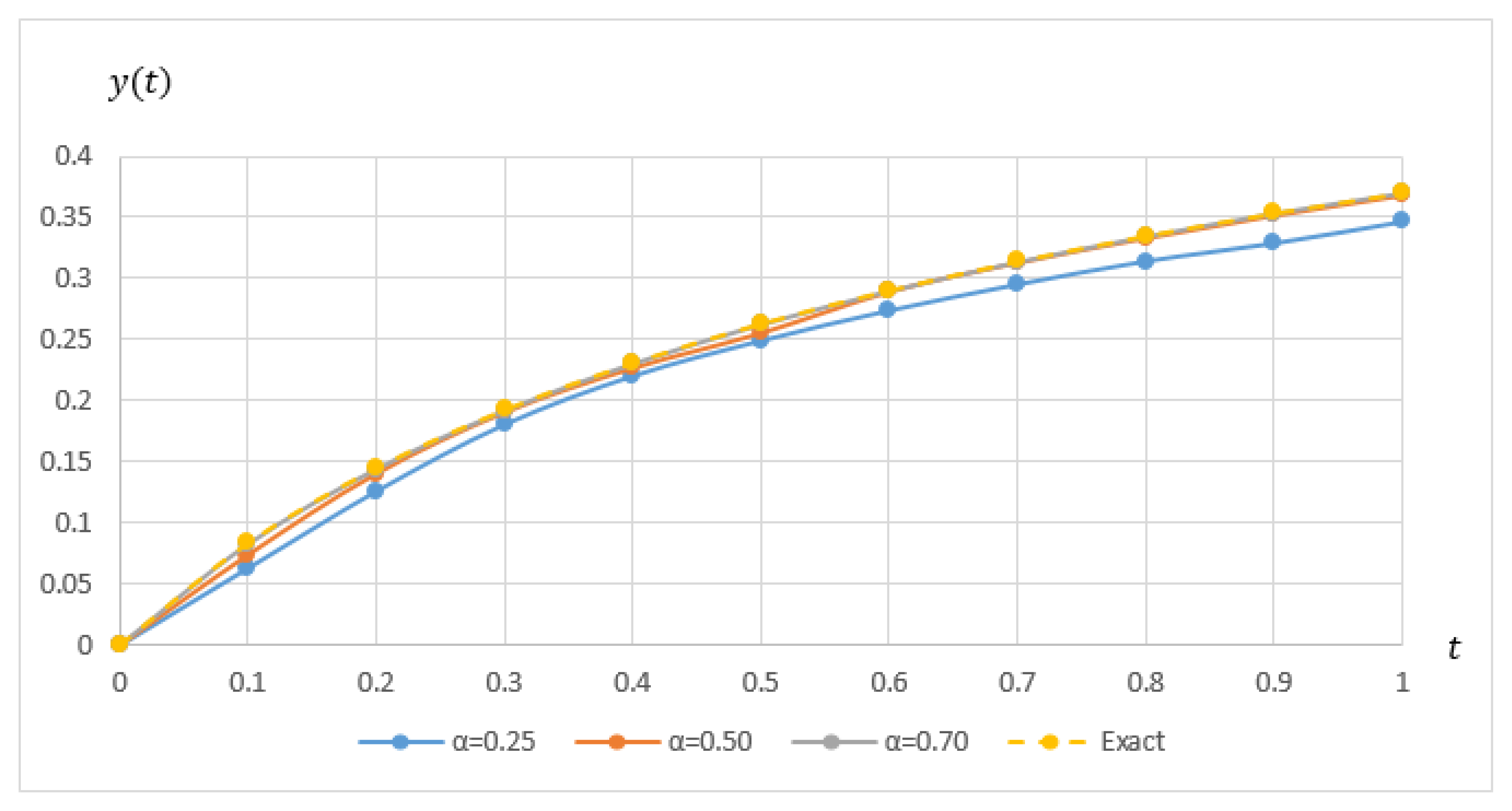
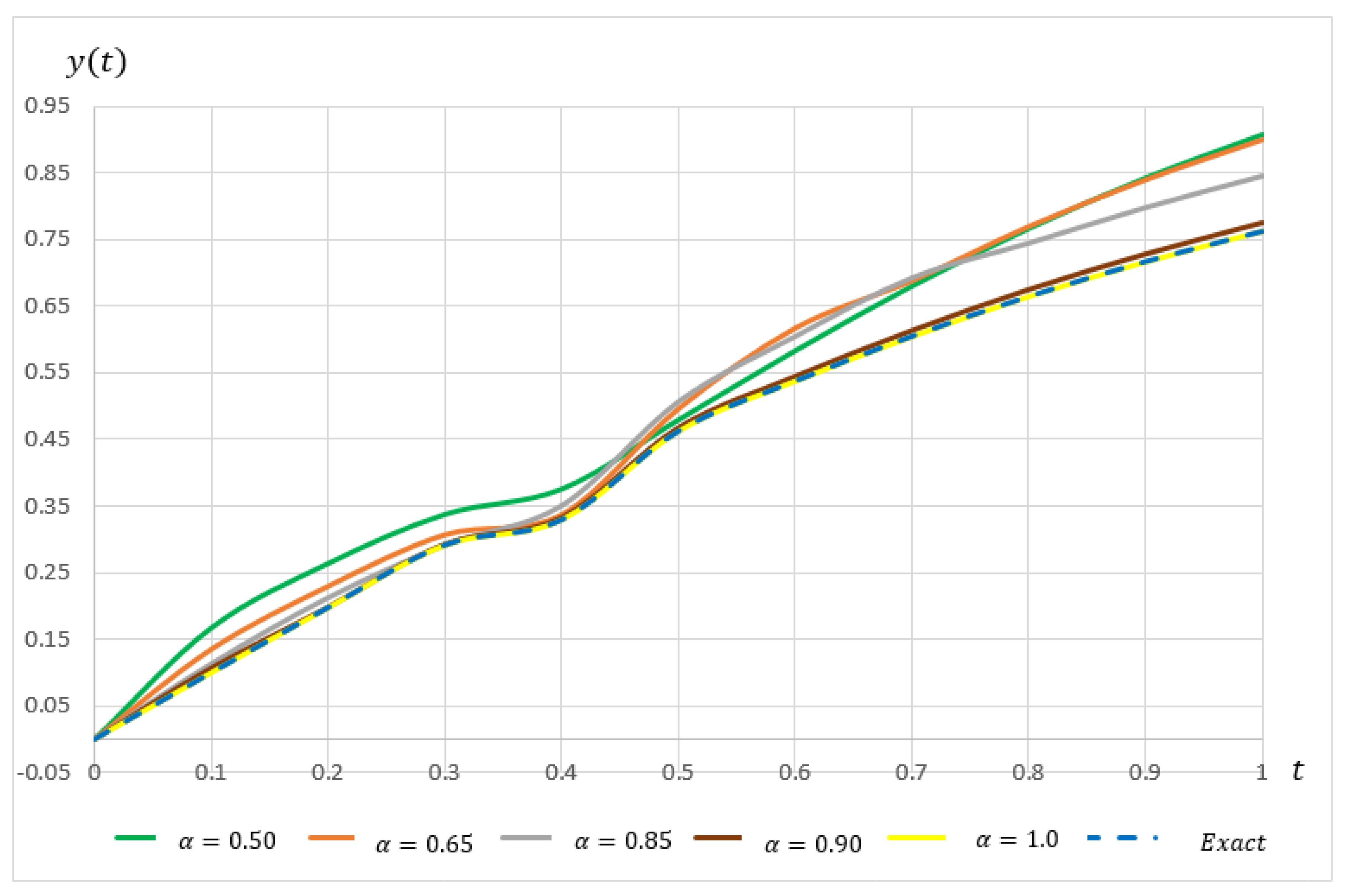
Next, Table 8 shows the numerical result for solving Example 4 when α = 1.0 , while Table 9 shows the results when α = 1.50 for solving Example 5. Both tables present the approximate solution and absolute errors at each point, t for different N. Based on these tables, it can be seen that better accuracy is obtained as N increases. For comparison purposes, Table 10 presents the comparison of absolute error between FEAM3 and SFMoPF at each point, t when α = 1.0 and N = 10 in solving Example 4, while Table 11 demonstrates the comparison of absolute error at each point, t between FEAM3 and 3-HOFLMSM in solving nonlinear higher order FDE of Example 5 when α = 1.50 and N = 100 . From these tables, the results given by FEAM3 are seen to be comparable to the respective existing methods. The performance graph for both examples are shown in Figure 8 and Figure 9, respectively, where, as α increases, the approximate solutions approach the exact solution.
This paper also includes solving fractional Riccati differential equation (FRDE). According to [30], it is well-known that the Riccati differential equation is concerned with applications in pattern formation in dynamic games, linear systems with Markovian jumps, diffusion problems, river flows, and econometric models. Therefore, many researchers have developed several analytical and numerical methods in solving FRDE problems, since it can be considered as one of the examples of application problems in FDE.
Table 12 presents the result on absolute error for solving FRDE problem by using FEAM3 at different intervals, N = 10 , 100 , 1000 when α = 1.0 . Based on the table, the absolute error for solving FRDE by using FEAM3 decreases as N increases. Thus, it gives meaning whereby, as the step size decreases, the approximate solutions approach the exact solutions. For comparison purposes, Table 13 shows the comparison result of solving the FRDE problem between FEAM3, FVIM, and MHPM when α = 1.0 and N = 10 . According to the table, FEAM3 managed to give a comparable result as FVIM and MHPM. Furthermore, a graph shows the approximate solution at each point, and t for solving the FRDE problem is also presented in Figure 10, where the approximate solutions do indeed approach the exact solution as α increases. Therefore, this implies that FEAM3 is able to perform well in solving nonlinear FDEs.
6. Conclusions

This paper has proposed a numerical method known as a fractional explicit Adams method of order 3, FEAM3. The numerical results obtained for each example authenticate that FEAM3 is adequate to preserve accuracy in solving both linear and nonlinear FDEs. The results also validate the convergence analysis where the approximate solutions are indeed converged and approach the exact solution as the step size, h, decreases. Additionally, FEAM3 is proven to be capable of achieving comparable results as the existing methods in each example. Furthermore, this paper also includes solving problems of FDE for the case of single and higher order, where the results have shown that the increment in the value of α yields better accuracy in solving both linear and nonlinear FDE problems. Therefore, it is proven that FEAM3 is competent and reliable to act as an alternative method to solve different kinds of FDEs.

Author Contributions

Formal analysis, Z.A.M.; Investigation, N.A.Z.; Methodology, N.A.Z.; Project administration, Z.A.M.; Resources, A.K. and F.R.; Supervision, Z.A.M.; Writing—original draft, N.A.Z.; Writing—review and editing, Z.A.M. All authors have read and agreed to the published version of the manuscript.

Funding

The authors gratefully acknowledge the financial support of Research University Grant (Putra Impact Grant: UPM/800-3/3/1/9629200) from Universiti Putra Malaysia.

Conflicts of Interest

The authors declare no conflict of interest.

References

  1. Assaleh, K.; Ahmad, W.M. Modeling of speech signals using fractional calculus. In Proceedings of the 2007 9th International Symposium on Signal Processing and Its Applications, Sharjah, UAE, 12–15 February 2007; pp. 1–4. [Google Scholar]
  2. Podlubny, I. Fractional-order systems and fractional-order controllers. Inst. Exp. Phys. Slovak Acad. Sci. Kosice 1994, 12, 1–18. [Google Scholar]
  3. Torvik, P.J.; Bagley, R.L. On the appearance of the fractional derivative in the behavior of real materials. J. Appl. Mech. 1984, 51, 294–298. [Google Scholar] [CrossRef]
  4. Olmstead, W.E.; Handelsman, R.A. Diffusion in a semi-infinite region with nonlinear surface dissipation. SIAM Rev. 1976, 18, 275–291. [Google Scholar] [CrossRef]
  5. Woon, S. Analytic continuation of operators applications: From number theory and group theory to quantum field and string theories. Rev. Math. Phys. 1999, 11, 463–501. [Google Scholar] [CrossRef]
  6. Bagley, R.L.; Torvik, P.J. On the fractional calculus model of viscoelastic behavior. J. Rheol. 1986, 30, 133–155. [Google Scholar] [CrossRef]
  7. Biala, T.A.; Jator, S.N. Block implicit Adams methods for fractional differential equations. Chaos Solitons Fractals 2015, 81, 365–377. [Google Scholar] [CrossRef]
  8. Garrappa, R. On some explicit Adams multistep methods for fractional differential equations. J. Comput. Appl. Math. 2009, 229, 392–399. [Google Scholar] [CrossRef] [Green Version]
  9. Kazem, S. Exact solution of some linear fractional differential equations by Laplace transform. Int. J. Nonlinear Sci. 2013, 16, 3–11. [Google Scholar]
  10. Li, C.; Tao, C. On the fractional Adams method. Comput. Math. Appl. 2009, 58, 1573–1588. [Google Scholar] [CrossRef] [Green Version]
  11. Eslahchi, M.R.; Dehghan, M.; Parvizi, M. Application of the collocation method for solving nonlinear fractional integro-differential equations. J. Comput. Appl. Math. 2014, 257, 105–128. [Google Scholar] [CrossRef]
  12. Wazwaz, A.M. The variational iteration method: A reliable analytic tool for solving linear and nonlinear wave equations. Comput. Math. Appl. 2007, 54, 926–932. [Google Scholar] [CrossRef] [Green Version]
  13. Khan, Y.; Faraz, N.; Yildirim, A.; Wu, Q. Fractional variational iteration method for fractional initial-boundary value problems arising in the application of nonlinear science. Comput. Math. Appl. 2011, 62, 2273–2278. [Google Scholar] [CrossRef] [Green Version]
  14. Liao, S. Homotopy analysis method: A new analytical technique for nonlinear problems. Commun. Nonlinear Sci. Numer. Simul. 1997, 2, 95–100. [Google Scholar] [CrossRef]
  15. Zurigat, M.; Momani, S.; Alawneh, A. Analytical approximate solutions of systems of fractional algebraic–differential equations by homotopy analysis method. Comput. Math. Appl. 2010, 59, 1227–1235. [Google Scholar] [CrossRef] [Green Version]
  16. Podlubny, I. Numerical solution of ordinary fractional differential equations by the fractional difference method. In Advances in Difference Equations: Proceedings of the Second International Conference on Difference Equations; Elaydi, S., Gyori, I., Ladas, G., Eds.; Gordon and Breach: Amsterdam, The Netherlands, 1997. [Google Scholar]
  17. Gorenflo, R. Fractional calculus: Some numerical methods. In Fractals and Fractional Calculus in Continuum Mechanics; Carpinteri, A., Mainardi, F., Eds.; Springer-Verlag: Vienna, Austria, 1997; pp. 277–290. [Google Scholar]
  18. Diethelm, K.; Ford, N.J.; Freed, A.D. A predictor–corrector approach for the numerical solution of fractional differential equations. Nonlinear Dyn. 2002, 29, 3–22. [Google Scholar] [CrossRef]
  19. Galeone, L.; Garrappa, R. On multistep methods for differential equations of fractional order. Mediterr. J. Math. 2006, 3, 565–580. [Google Scholar] [CrossRef]
  20. Błaszczyk, T.; Leszczyński, J.S. Using the Euler’s method to solve ordinary differential equations of higher order with a mixture of integer and Caputo derivatives. Sci. Res. Inst. Math. Comput. Sci. 2007, 6, 31–40. [Google Scholar]
  21. Diethelm, K.; Ford, N.J.; Freed, A.D. Detailed error analysis for a fractional Adams method. Numer. Algorithms 2004, 36, 31–52. [Google Scholar] [CrossRef] [Green Version]
  22. Diethelm, K. The Analysis of Fractional Differential Equations: An Application-Oriented Exposition Using Differential Operators of Caputo Type; Springer-Verlag: Berlin/Heidelberg, Germany, 2010. [Google Scholar]
  23. Gnitchogna, R.; Atangana, A. New two step Laplace Adam–Bashforth method for integer a noninteger order partial differential equations. Numer. Methods Partial Differ. Equ. 2018, 34, 1739–1758. [Google Scholar] [CrossRef] [Green Version]
  24. Lambert, J.D. Computational Methods in Ordinary Differential Equations; Wiley: Hoboken, NJ, USA, 1973. [Google Scholar]
  25. Bonab, Z.F.; Javidi, M. Higher order methods for fractional differential equation based on fractional backward differentiation formula of order three. Math. Comput. Simul. 2020, 172, 71–89. [Google Scholar] [CrossRef]
  26. Biala, T.A.; Jator, S.N. Block backward differentiation formulas for fractional differential equations. Int. J. Eng. Math. 2015, 2015, 650425. [Google Scholar] [CrossRef]
  27. Ahmed, H. Fractional Euler method; an effective tool for solving fractional differential equations. J. Egypt. Math. Soc. 2018, 26, 38–43. [Google Scholar] [CrossRef] [Green Version]
  28. Al-Rabtah, A.; Momani, S.; Ramadan, M.A. Solving linear and nonlinear fractional differential equations using spline functions. Abstr. Appl. Anal. 2012, 2012, 426514. [Google Scholar] [CrossRef] [Green Version]
  29. Lin, R.; Liu, F. Fractional high order methods for the nonlinear fractional ordinary differential equation. Nonlinear Anal. Theory Methods Appl. 2007, 66, 856–869. [Google Scholar] [CrossRef] [Green Version]
  30. Merdan, M. On the solutions fractional Riccati differential equation with modified Riemann–Liouville derivative. Int. J. Differ. Equ. 2012, 2012, 346089. [Google Scholar] [CrossRef]
  31. Odibat, Z.; Momani, S. Modified homotopy perturbation method: Application to quadratic Riccati differential equation of fractional order. Chaos Solitons Fractals 2008, 36, 167–174. [Google Scholar] [CrossRef]
Figure 1. Stability region for FEAM3 when 0 < α < 1 .
Mathematics 08 01675 g001
Figure 2. Stability region of FEAM3 for different values of α .
Mathematics 08 01675 g002
Figure 3. Stability region for FEAM3 when 1 < α < 2 .
Mathematics 08 01675 g003
Figure 4. Approximate solution, y ( t ) against each point, t at different N of α = 0.50 when solving Example 1 using FEAM3.
Mathematics 08 01675 g004
Figure 5. Approximate solution, y ( t ) against each point, t at different N of α = 1.50 when solving Example 1 using FEAM3.
Mathematics 08 01675 g005
Figure 6. Approximate solution, y ( t ) against each point, t at different N of α = 0.50 when solving Example 2 using FEAM3.
Mathematics 08 01675 g006
Figure 7. Approximate solution, y ( t ) against each point, t at different N of α = 1.50 when solving Example 3 using FEAM3.
Mathematics 08 01675 g007
Figure 8. Approximate solution, y ( t ) against each point, t of different α at N = 100 when solving Example 4 using FEAM3.
Mathematics 08 01675 g008
Figure 9. Approximate solution, y ( t ) against each point, t of different α at N = 100 when solving Example 5 using FEAM3.
Mathematics 08 01675 g009
Figure 10. Approximate solution, y ( t ) against each point, t of different α at N = 100 when solving Example 6 using FEAM3.
Mathematics 08 01675 g010
Table 1. Absolute error at each point, t when solving Example 1 using FEAM3 for different step size, h and 0 < α < 1 .
t α = 0.30 α = 0.50 α = 0.70
h = 10 3 h = 10 4 h = 10 3 h = 10 4 h = 10 3 h = 10 4
0.1 9.5771 × 10 4 9.6093 × 10 5 9.8712 × 10 4 9.8749 × 10 5 9.9312 × 10 5 9.9322 × 10 7
0.2 8.9823 × 10 4 9.0141 × 10 5 9.5845 × 10 4 9.5881 × 10 5 9.7441 × 10 5 9.7451 × 10 7
0.3 8.4558 × 10 4 8.3493 × 10 5 9.2038 × 10 4 9.1833 × 10 5 9.4583 × 10 5 9.4511 × 10 6
0.4 7.7652 × 10 4 7.6492 × 10 5 8.7032 × 10 4 8.6814 × 10 5 9.0656 × 10 5 9.0580 × 10 6
0.5 7.0663 × 10 4 6.9359 × 10 5 8.1225 × 10 4 8.0986 × 10 6 8.5816 × 10 5 8.5735 × 10 6
0.6 6.3651 × 10 4 6.2332 × 10 5 7.4739 × 10 5 7.4512 × 10 6 8.0133 × 10 5 8.0056 × 10 6
0.7 5.6741 × 10 4 5.5624 × 10 5 6.7702 × 10 5 6.7537 × 10 6 7.3689 × 10 5 7.3631 × 10 6
0.8 4.9984 × 10 4 4.9146 × 10 5 6.0223 × 10 5 6.0077 × 10 6 6.6562 × 10 5 6.6514 × 10 6
0.9 4.3429 × 10 4 4.2664 × 10 5 5.2409 × 10 5 5.2357 × 10 6 7.8838 × 10 6 5.8820 × 10 6
1.0 3.7122 × 10 4 3.7096 × 10 5 4.4374 × 10 5 4.4911 × 10 6 7.0611 × 10 6 5.0829 × 10 6
Table 2. Absolute error at each point, t when solving Example 1 using FEAM3 for different step size, h and 1 < α < 2 .
t α = 1.30 α = 1.70 α = 1.90
h = 10 3 h = 10 4 h = 10 3 h = 10 4 h = 10 3 h = 10 4
0.1 1.9057 × 10 4 3.4686 × 10 4 8.0403 × 10 6 2.1789 × 10 6 2.8747 × 10 6 1.2469 × 10 7
0.2 3.8632 × 10 4 4.3643 × 10 4 2.3011 × 10 5 3.3239 × 10 6 1.0539 × 10 6 2.5204 × 10 7
0.3 4.6840 × 10 4 5.0529 × 10 4 3.3214 × 10 5 2.7909 × 10 6 2.4354 × 10 6 1.5195 × 10 7
0.4 4.7932 × 10 4 4.7977 × 10 5 4.2204 × 10 5 8.4032 × 10 6 4.7842 × 10 6 8.4336 × 10 7
0.5 5.3807 × 10 4 4.2912 × 10 5 4.6650 × 10 5 4.1940 × 10 6 4.8808 × 10 6 6.1950 × 10 7
0.6 5.5647 × 10 4 3.0905 × 10 5 4.7572 × 10 5 1.8945 × 10 6 4.7271 × 10 6 1.9682 × 10 7
0.7 5.6654 × 10 4 5.3644 × 10 5 4.6364 × 10 5 6.9250 × 10 6 4.4137 × 10 7 5.8584 × 10 7
0.8 5.6382 × 10 4 1.3530 × 10 6 4.4518 × 10 5 2.6724 × 10 6 4.1039 × 10 7 1.8696 × 10 7
0.9 5.6442 × 10 4 6.6676 × 10 6 4.2753 × 10 5 1.1572 × 10 7 3.8147 × 10 7 6.6892 × 10 8
1.0 6.7363 × 10 5 3.1084 × 10 6 4.1161 × 10 5 5.6829 × 10 7 3.5291 × 10 7 2.7141 × 10 8
Table 3. Absolute error at point, t = 1 when solving Example 1 using FEAM3 and FAM for different values of α and N.
N α = 0.10 α = 0.90 α = 1.25 α = 1.85
FAMFEAM3FAMFEAM3FAMFEAM3FAMFEAM3
105.4200 × 10 3 4.8546 × 10 4 7.5100 × 10 4 2.8304 × 10 4 5.6100 × 10 4 2.7017 × 10 4 4.4000 × 10 4 3.9235 × 10 5
201.2200 × 10 3 2.0575 × 10 4 1.9100 × 10 4 1.1861 × 10 4 1.2700 × 10 4 3.4704 × 10 4 1.0700 × 10 4 2.2228 × 10 5
404.4000 × 10 4 1.4901 × 10 4 4.9900 × 10 5 2.2551 × 10 5 2.9000 × 10 5 1.5263 × 10 5 2.6500 × 10 5 1.1438 × 10 6
801.6800 × 10 4 1.9998 × 10 4 1.3200 × 10 5 1.3469 × 10 5 6.6800 × 10 6 5.0983 × 10 5 6.5700 × 10 6 8.3091 × 10 6
1606.6500 × 10 5 3.2164 × 10 5 3.5400 × 10 6 2.8719 × 10 6 1.5500 × 10 6 1.3484 × 10 6 1.6300 × 10 6 3.3188 × 10 7
3202.6800 × 10 5 1.1752 × 10 5 9.4800 × 10 7 3.4023 × 10 6 3.6300 × 10 7 3.6436 × 10 6 4.0700 × 10 7 1.8543 × 10 7
Table 4. Absolute error at each point, t when solving Example 2 using FEAM3 for different step size, h and 0 < α < 1 .
t α = 0.30 α = 0.50 α = 0.90
h = 10 3 h = 10 4 h = 10 3 h = 10 4 h = 10 3 h = 10 4
0.1 1.4849 × 10 2 2.8244 × 10 3 9.0000 × 10 4 1.2241 × 10 4 2.9811 × 10 5 2.2241 × 10 7
0.2 6.3986 × 10 3 3.0468 × 10 3 4.9629 × 10 4 1.3897 × 10 4 2.4031 × 10 5 2.7738 × 10 7
0.3 1.3939 × 10 2 3.2018 × 10 3 8.9975 × 10 4 1.5745 × 10 4 3.4758 × 10 5 3.5718 × 10 7
0.4 1.4322 × 10 2 3.3674 × 10 3 9.4321 × 10 4 1.7734 × 10 4 3.6749 × 10 5 4.5838 × 10 7
0.5 1.4512 × 10 2 3.5558 × 10 3 9.6502 × 10 4 1.9881 × 10 4 3.7973 × 10 5 5.7889 × 10 7
0.6 1.4736 × 10 2 3.7945 × 10 3 9.8398 × 10 4 2.2259 × 10 4 3.9062 × 10 5 7.1756 × 10 7
0.7 1.5078 × 10 2 4.0999 × 10 3 1.0060 × 10 3 2.4936 × 10 4 4.0196 × 10 5 8.7389 × 10 7
0.8 1.5508 × 10 2 4.4709 × 10 3 1.0322 × 10 3 2.7978 × 10 4 4.1447 × 10 5 1.0479 × 10 6
0.9 1.5946 × 10 2 4.8778 × 10 3 1.0613 × 10 3 3.1344 × 10 4 4.2842 × 10 5 1.2395 × 10 6
1.0 1.6321 × 10 2 5.2439 × 10 3 1.0907 × 10 3 3.4778 × 10 4 4.4381 × 10 5 1.4474 × 10 6
Table 5. Absolute error at t = 1 at different α and step size, h using FEAM3 and FLMM-3 in solving Example 2.
h α = 0.7 α = 0.8
FEAM3FLMM-3FEAM3FLMM-3
0.1 2.4399 × 10 3 1.8400 × 10 2 9.8785 × 10 3 1.3500 × 10 2
0.01 7.1853 × 10 4 4.4733 × 10 4 2.0451 × 10 4 3.0718 × 10 4
0.001 6.8739 × 10 5 9.3791 × 10 6 1.9192 × 10 5 5.4728 × 10 6
Table 6. Absolute error at each point, t when solving Example 3 by using FEAM3 for different step size, h and 1 < α < 2 .
t α = 1.30 α = 1.70 α = 1.90
h = 10 3 h = 10 4 h = 10 3 h = 10 4 h = 10 3 h = 10 4
0.1 1.1270 × 10 6 2.6967 × 10 7 7.1098 × 10 8 9.5528 × 10 9 2.8292 × 10 8 2.0712 × 10 9
0.2 1.6199 × 10 6 2.6204 × 10 7 1.2859 × 10 7 9.7208 × 10 9 7.6637 × 10 8 2.0667 × 10 9
0.3 4.0534 × 10 7 2.5826 × 10 7 1.2427 × 10 7 1.1881 × 10 8 7.5718 × 10 8 2.1642 × 10 9
0.4 9.4156 × 10 6 2.7676 × 10 7 1.1910 × 10 7 1.9696 × 10 8 7.5543 × 10 8 2.7266 × 10 8
0.5 8.7041 × 10 6 3.2962 × 10 7 1.1507 × 10 7 3.2683 × 10 8 8.0033 × 10 8 3.8727 × 10 8
0.6 9.0579 × 10 6 3.6668 × 10 7 1.1512 × 10 7 2.9013 × 10 8 8.8761 × 10 8 3.3980 × 10 8
0.7 9.2041 × 10 6 8.5859 × 10 8 1.1223 × 10 7 6.7724 × 10 8 6.8659 × 10 8 7.6489 × 10 8
0.8 9.1149 × 10 6 1.1897 × 10 7 6.8416 × 10 8 4.3546 × 10 8 1.0618 × 10 8 5.1537 × 10 8
0.9 5.9700 × 10 6 3.6511 × 10 7 1.2468 × 10 7 1.3654 × 10 8 7.5398 × 10 7 1.6554 × 10 8
1.0 4.5348 × 10 6 1.0675 × 10 7 7.1850 × 10 7 3.1913 × 10 8 2.4646 × 10 8 3.8947 × 10 9
Table 7. Absolute error when α = 1.25 at different step size, h using FEAM3 and ATPC in solving Example 3.
h α = 1.25
FEAM3ATPC
1 / 10 1.5273 × 10 3 5.5300 × 10 3
1 / 20 5.8067 × 10 4 1.5900 × 10 3
1 / 40 8.5459 × 10 5 4.3300 × 10 4
1 / 80 1.2959 × 10 5 1.1400 × 10 4
1 / 160 5.4481 × 10 6 2.9700 × 10 5
1 / 320 2.2915 × 10 6 7.6600 × 10 6
1 / 640 6.9897 × 10 6 1.9600 × 10 6
Table 8. Approximate solutions and absolute errors at each point, t when α = 1.0 for solving Example 4 by using FEAM3 at different intervals, N.
tExactN = 10N = 100N = 1000
Approx.ErrorApprox.ErrorApprox.Error
0.0 1.0000 × 10 0 1.0000 × 10 0 0.0000 × 10 0 1.0000 × 10 0 0.0000 × 10 0 1.0000 × 10 0 0.0000 × 10 0
0.1 8.3756 × 10 2 8.2805 × 10 2 9.1624 × 10 5 7.6591 × 10 2 9.5393 × 10 6 8.3034 × 10 2 2.0646 × 10 7
0.2 1.4504 × 10 1 1.4551 × 10 1 8.5496 × 10 5 1.3962 × 10 1 4.3778 × 10 6 1.4448 × 10 1 2.9003 × 10 7
0.3 1.9265 × 10 1 1.4567 × 10 1 8.0735 × 10 5 1.8833 × 10 1 1.8424 × 10 7 1.9219 × 10 1 7.1961 × 10 7
0.4 2.3116 × 10 1 1.9381 × 10 1 7.6884 × 10 5 2.2761 × 10 1 4.1394 × 10 6 2.3077 × 10 1 1.0895 × 10 6
0.5 2.6324 × 10 1 2.3246 × 10 1 7.3676 × 10 5 2.6024 × 10 1 7.5527 × 10 6 2.6289 × 10 1 1.4060 × 10 6
0.6 2.9056 × 10 1 2.6453 × 10 1 7.0944 × 10 5 2.8797 × 10 1 1.0483 × 10 5 2.9026 × 10 1 1.6752 × 10 6
0.7 3.1423 × 10 1 2.9179 × 10 1 6.8577 × 10 5 3.1196 × 10 1 1.2981 × 10 5 3.1396 × 10 1 1.9021 × 10 6
0.8 3.3503 × 10 1 3.1539 × 10 1 6.6498 × 10 5 3.3302 × 10 1 1.5097 × 10 5 3.3478 × 10 1 2.0914 × 10 6
0.9 3.5351 × 10 1 3.3610 × 10 1 6.4649 × 10 4 3.5171 × 10 1 1.6871 × 10 5 3.5328 × 10 1 2.2475 × 10 6
1.0 3.7009 × 10 1 3.5451 × 10 1 6.2990 × 10 4 3.6847 × 10 1 1.8343 × 10 5 3.6988 × 10 1 2.3741 × 10 6
Table 9. Approximate solutions and absolute errors at each point, t when α = 1.50 for solving Example 5 by using FEAM3 at different intervals, N.
tExactN = 10N = 1000N = 10,000
Approx.ErrorApprox.ErrorApprox.Error
0.0 0.0000 × 10 0 0.0000 × 10 0 0.0000 × 10 0 0.0000 × 10 0 0.0000 × 10 0 0.0000 × 10 0 0.0000 × 10 0
0.2 1.1520 × 10 2 4.5689 × 10 2 4.5689 × 10 2 1.1518 × 10 2 1.9701 × 10 6 1.1520 × 10 2 1.5952 × 10 8
0.4 6.1440 × 10 2 5.8370 × 10 2 3.0699 × 10 3 6.1431 × 10 2 8.8948 × 10 6 6.1440 × 10 2 7.4729 × 10 8
0.6 1.2096 × 10 1 1.1856 × 10 1 2.3959 × 10 3 1.2095 × 10 1 9.1466 × 10 6 1.2095 × 10 1 2.7482 × 10 7
0.8 1.2288 × 10 1 1.2003 × 10 1 2.8521 × 10 3 1.2287 × 10 1 1.1237 × 10 6 1.2288 × 10 1 8.1659 × 10 7
1.0 0.0000 × 10 0 2.4589 × 10 3 2.4589 × 10 3 2.1086 × 10 6 2.1086 × 10 6 1.0322 × 10 6 1.0322 × 10 6
1.2 −2.7648 × 10 1 −2.7182 × 10 1 4.6558 × 10 3 −2.7648 × 10 1 4.2249 × 10 6 −2.7648 × 10 1 2.7720 × 10 6
1.4 −6.5856 × 10 1 −6.9174 × 10 1 3.3179 × 10 2 −6.5857 × 10 1 5.8588 × 10 6 −6.5856 × 10 1 1.5672 × 10 6
1.6 −9.8304 × 10 1 −9.9521 × 10 1 1.2165 × 10 2 −9.8305 × 10 1 1.0593 × 10 5 −9.8305 × 10 1 1.1164 × 10 5
1.8 −9.3312 × 10 1 −9.6244 × 10 1 2.9316 × 10 2 −9.3314 × 10 1 1.7703 × 10 5 −9.3314 × 10 1 1.8906 × 10 5
2.0 0.0000 × 10 0 1.8550 × 10 2 1.8550 × 10 2 2.2301 × 10 5 2.2301 × 10 5 6.3499 × 10 5 6.3499 × 10 5
Table 10. Absolute error when α = 1.0 at each point, t using FEAM3 with N = 10 and SFMoPF in solving Example 4.
tExact α = 1.0
FEAM3SFMoPF
0.1 8.3756 × 10 2 9.1624 × 10 5 9.3660 × 10 5
0.2 1.4504 × 10 1 8.5496 × 10 5 1.1397 × 10 4
0.3 1.9381 × 10 1 8.0735 × 10 5 1.1162 × 10 4
0.4 2.3116 × 10 1 7.6884 × 10 5 1.0297 × 10 4
0.5 2.6324 × 10 1 7.3676 × 10 5 9.3223 × 10 5
0.6 2.9056 × 10 1 7.0944 × 10 5 8.4033 × 10 5
0.7 3.1423 × 10 1 6.8577 × 10 5 7.5850 × 10 5
0.8 3.3503 × 10 1 6.6497 × 10 5 6.8710 × 10 5
0.9 3.5351 × 10 1 6.4649 × 10 4 6.2520 × 10 5
1.0 3.7009 × 10 1 6.2990 × 10 4 5.7152 × 10 5
Table 11. Absolute error when α = 1.50 and N = 100 at each point, t using FEAM3 and 3-HOFLMSM in solving Example 5.
t α = 1.50
FEAM33-HOFLMSM
0.2 1.5523 × 10 6 3.2219 × 10 6
0.4 6.2872 × 10 6 2.9192 × 10 5
0.6 6.3215 × 10 6 3.9717 × 10 5
0.8 5.3296 × 10 5 3.4898 × 10 5
1.0 3.4589 × 10 5 1.5445 × 10 5
1.2 2.5296 × 10 5 1.8140 × 10 5
1.4 9.4439 × 10 5 6.8333 × 10 5
1.6 4.0478 × 10 4 1.4371 × 10 4
1.8 2.2499 × 10 4 2.5759 × 10 4
2.0 2.2998 × 10 4 4.0599 × 10 4
Table 12. Absolute error at each point, t in solving Example 6 by using FEAM3 when α = 1.0 for different values of N.
t α = 1.00
N = 10N = 100N = 1000
0.00.0000 × 10 0 0.0000 × 10 0 0.0000 × 10 0
0.13.3201 × 10 6 1.9293 × 10 7 5.0289 × 10 8
0.21.6247 × 10 6 3.7449 × 10 6 1.0653 × 10 7
0.31.3343 × 10 5 9.0931 × 10 6 1.5932 × 10 7
0.45.3423 × 10 4 1.3975 × 10 5 2.0725 × 10 6
0.54.9208 × 10 4 1.8286 × 10 5 2.4929 × 10 6
0.64.5129 × 10 4 2.1961 × 10 5 2.8479 × 10 6
0.73.9082 × 10 4 2.4971 × 10 5 3.1351 × 10 6
0.83.3488 × 10 4 2.7323 × 10 5 3.3549 × 10 6
0.92.8359 × 10 4 2.9049 × 10 5 3.5108 × 10 6
1.02.3869 × 10 4 3.0198 × 10 5 3.6079 × 10 6
Table 13. Approximate solution and absolute error at each point, t when α = 1.0 with N = 10 in solving Example 6 by using FEAM3 compared to previous methods, FVIM and MHPM.
tExactFVIMMHPMFEAM3
Approx.ErrorApprox.ErrorApprox.Error
0.0 0.0000 × 10 0 0.0000 × 10 0 0.0000 × 10 0 0.0000 × 10 0 0.0000 × 10 0 0.0000 × 10 0 0.0000 × 10 0
0.1 9.9667 × 10 2 9.9967 × 10 2 0.0000 × 10 0 9.9667 × 10 2 0.0000 × 10 0 9.9966 × 10 2 3.3201 × 10 6
0.2 1.9738 × 10 1 1.9738 × 10 1 0.0000 × 10 0 1.9738 × 10 1 0.0000 × 10 0 1.9737 × 10 1 1.6247 × 10 6
0.3 2.9131 × 10 1 2.9132 × 10 1 8.0000 × 10 6 2.9131 × 10 1 0.0000 × 10 0 2.9131 × 10 1 1.3343 × 10 5
0.4 3.7995 × 10 1 3.8001 × 10 1 5.7000 × 10 5 3.7994 × 10 1 4.0000 × 10 6 3.7995 × 10 1 5.3423 × 10 4
0.5 4.6212 × 10 1 4.6234 × 10 1 2.5800 × 10 4 4.6208 × 10 1 3.9000 × 10 5 4.6212 × 10 1 4.9208 × 10 4
0.6 5.3705 × 10 1 5.3792 × 10 1 8.7400 × 10 4 5.3686 × 10 1 1.9200 × 10 4 5.3702 × 10 1 4.5129 × 10 4
0.7 6.0437 × 10 1 6.0677 × 10 1 2.4010 × 10 3 6.0363 × 10 1 7.3600 × 10 4 6.0434 × 10 1 3.9082 × 10 4
0.8 6.6404 × 10 1 6.6970 × 10 1 5.6590 × 10 3 6.6171 × 10 1 2.3300 × 10 3 6.6401 × 10 1 3.3488 × 10 4
0.9 7.1630 × 10 1 7.2814 × 10 1 1.1842 × 10 2 7.0992 × 10 1 6.3780 × 10 3 7.1626 × 10 1 2.8359 × 10 4
1.0 7.6159 × 10 1 7.8413 × 10 1 2.2532 × 10 2 7.4603 × 10 1 1.5562 × 10 2 7.6155 × 10 1 2.3869 × 10 4