Differential Evolution for Neural Networks Optimization

Abstract

In this paper, a Neural Networks optimizer based on Self-adaptive Differential Evolution is presented. This optimizer applies mutation and crossover operators in a new way, taking into account the structure of the network according to a per layer strategy. Moreover, a new crossover called interm is proposed, and a new self-adaptive version of DE called MAB-ShaDE is suggested to reduce the number of parameters. The framework has been tested on some well-known classification problems and a comparative study on the various combinations of self-adaptive methods, mutation, and crossover operators available in literature is performed. Experimental results show that DENN reaches good performances in terms of accuracy, better than or at least comparable with those obtained by backpropagation.

1. Introduction

The use of Neural Network (NN) models has been steadily increasing in the recent past, following the introduction of Deep Learning methods and the ever-growing computational capabilities of modern machines. Thus, such models are applied to various problems, including image classification [1] and generation [2], text classification [3], speech recognition [4], emotion recognition [5], and many more. New and more complex network structures, such as Convolutional Neural Networks [6], Neural Turing Machines [7], and NRAM [8], were developed and applied to the aforementioned tasks; such new problems and structures also required the development of new optimization techniques [9,10,11].

According to these new trends, neuroevolution has also been renewed [12,13,14,15]. The term of neuroevolution is used to identify the research area where evolutionary algorithms are used to construct and train artificial neural networks. Several approaches have been proposed both to train networks’ weights and topology and to exploit the characteristics of neuroevolution of being highly general, allowing learning with nondifferentiable activation functions, without explicit targets, and with recurrent networks [16,17].

The traditional method used by neural networks to learn their weights and biases is the gradient descent algorithm applied to a cost function and its most famous implementation is the backpropagation procedure. Nowadays, the backpropagation algorithm is still the workhorse of learning in neural networks even if its origin dates back to 1970s; its importance was revealed in 1986 [18].

Backpropagation works under two main assumptions about the form of the cost function: it has to be written as an average over cost functions $C_x$ for individual training examples x and as a function of the outputs from the neural network. Moreover the activation functions have to be differentiable.

With that said, there are tricks for avoiding this kind of problems, and finding alternatives to gradient descent is an active area of investigation. An interesting analysis on the motivations according to backpropagation is the most used technique based on gradient to train neural networks and evolutionary approaches are not sufficiently studied is presented in [15].

As long as meta-heuristic algorithms are generally nondeterministic and not sensitive to the differentiability and continuity of the objective functions, these methods are used in a wide range of complex optimization problems. In addition, the stochastic global optimizations can identify global minimum without being trapped in local minima [19,20,21].

The most used evolutionary approach in neuroevolution is the genetic one, extensively employed in the conventional neuroevolution (CNE) [17,22] and also recently proposed in the case of deep neuroevolution [23]. In those algorithms, the best individuals (the individuals with the highest fitness) are evolved by means of the mutation and crossover operators and replace the genotypes with the lowest fitness in the population. The genetic approach is the most used technique because it is easy to implement and practical in many domains. However, on the other hand, there is the problem of the encoding since they use a discrete optimization method to solve continuous problems.

In order to avoid the encoding problem other continuous evolutionary meta-algorithms have been proposed including, in particular, differential evolution (DE). Indeed, DE evolves a population of real-valued vectors, so no encoding and decoding are required.

It is well known that DE performs better than other popular evolutionary algorithms [24], has a quick convergence, and is robust [25]; it also performs better for learning applications [26]. At the same time, DE has simple genetic operations, such as its operator of the mutation and survival strategy based on one-on-one competition. Moreover, they can also use population global information and individual local information to search for the optimal solution.

When the optimization problem is complex, the performance of the traditional DE algorithm depends on the selected the control parameters and mutation strategy [19,27,28,29]. If the control parameters and selected mutation strategy are unsuitable, then DE is likely to yield premature convergence, stagnation phenomena and excessive consumption of computational resources. In particular, the stagnation problem for DE applied to neural network optimization has been studied in [30].

In this paper the system DENN that optimizes artificial Neural Networks using DE is presented. The system uses a direct encoding with a one-to-one mapping between the weights of the neural networks and values of individuals in the population. This system is an enhanced version of the system introduced in [12], where a preliminary implementation was described.

A batching system is introduced to overcome one of the main computational problems of the proposed approach, i.e., the fitness computation. For every generation the population is evaluated on a limited number of training examples, given by the size of the current batch, rather than the whole training set. This reduces the computational load, particularly on large training sets. Moreover, a restart method is applied to avoid a premature convergence of the algorithm: the best individual is saved and the rest of the current population is discarded, continuing the research on a new random generated population.

Finally, a new self-adaptive mutation strategy MAB-ShaDE inspired to the multi-armed bandit UCB1 [31] and a new particular crossover operator interm, a randomized version of the arithmetic crossover, have been proposed.

An extensive experimental study have been implemented to (i) determine if this approach is scalable and applicable also to large classification problems, like MNIST digit recognition; (ii) study the performance reached by using MAB-ShaDE and interm components; and (iii) identify the best algorithm configurations, i.e., the configurations reaching the highest accuracy.

The experimental results show that DENN is able to outperform the backpropagation algorithm in training neural networks without hidden layers. Moreover, DENN is a viable solution also from a computational point of view, even if the time spent for learning is higher than its competitor BPG.

The paper is organized as follows. Background concepts about neuroevolution, DE algorithm and its self-adaptive strategies are summarized in Section 2, related works are presented in Section 3, the system is presented in Section 4, and experimental results are shown in Section 5. Section 6 closes the paper with some final considerations and some ideas for future works.

2. Background

2.1. Differential Evolution

Differential evolution (DE) is a evolutionary algorithm used for optimization over continuous spaces, which operates by improving a population of N candidate solutions evaluated by means of a fitness function f though a iterative process. The first phase is the initialization in which the first population is generated; there exists various approaches, among which the most common is randomly generating each vector. Following, during the iterative phase, for each generation a new population is computed though mutation and crossover operators; each new vector is evaluated and then the best ones are chosen, according to a selection operator, for the next generation. The evolution may proceed for a fixed number of generations or until a given criterion is met.

The mutation used in DE is called differential mutation. For each vector target vector $x_i$, for $i=1,\dots ,N$, of the current generation, a vector ${\overline{y}}_i$, namely, donor vector, is calculated as linear combination of some vectors in the DE population selected according to a given strategy. In the literature, there exist many variants of the mutation operator (see for instance [32]). In this work, we implemented and used three operators: rand/1 [33], current_to_pbest [34], and DEGL [35].

The operator rand/1 is defined as

$${\overline{y}}_i=x_a+F(x_b-x_c)$$

(1)

where $F\in [0,2]$ is a real parameter called mutation Factor, $a,b,c$ are unique random indices different from i.

The operator curr_to_pbest is defined as

$${\overline{y}}_i=x_i+F(x_{pbest}-x_i)+F(x_a-x_b)$$

(2)

where $p\in \left(0,1\right]$ and $pbest$ is randomly selected index from the indices of the best $N\times p$ individuals of the population. Moreover, $x_b$ is an individual randomly chosen from the set

$$\{x_1,\dots ,x_N\}\setminus \{x_a,x_i\}\cup \mathcal{A}$$

where $\mathcal{A}$ is an external archive of bounded size (usually with at most N individuals) that contains the individuals discarded by the selection operator.

Finally, DEGL is defined as

$$\left\{\begin{array}{l}{\overline{y}}_i=w{L}_i+(1-w)G_i\hfill \\ L_i=x_i+\alpha (x_{nnbest}-x_i)+\beta (x_a-x_b)\hfill \\ G_i=x_i+\alpha (x_{best}-x_i)+\beta (x_a-x_b)\hfill \end{array}\right.$$

(3)

where $best$ is the index of the best individual in the population, $nnbest$ is the index of the best individual in the neighborhood of the target $x_i$, and $w\in \left[0,1\right]$ is the weight of the convex combination between $L_i$ and $G_i$.

The crossover operator creates a new vector $y_i$, namely trial vector, by recombining the donor with the corresponding target vector. There are many kinds of crossover; the most known is the binomial crossover where $y_i$ is computed as follows,

$$y_{i,j}=\left\{\begin{array}{ll}{\overline{y}}_{i,j}\hfill & \mathrm{if}ran{d}_{i,j}\le CR\mathrm{or}j=j_{rand}\hfill \\ x_{i,j}\hfill & \mathrm{otherwise}\hfill \end{array}\right.\mathrm{for}j=1,\dots ,D$$

(4)

where $ran{d}_{i,j}\in \left[0,1\right]$ is a real random number in $[0,1]$, $j_{rand}$ is an integer random number in $\{1,\dots ,D\}$, and $CR\in \left[0,1\right]$ is the crossover probability.

Finally, the selection operator compares each trial vector $y_i$ with the corresponding target vector $x_i$ and selects the better of them in the population of the next generation.

2.1.1. Self-Adaptive Differential Evolution

The DE parameters F and $CR$ have a strong impact during the evolution and the choose of their values is hard. In literature there exist many proposals of self-adaptive methods that select the values for F and $CR$.

One of the simplest and most popular method is jDE [36]. Each population individual $x_i$ has its own values $F_i$ and $C{R}_i$. The trial individual $z_i$ inherits from the target the values $F_i$ and $C{R}_i$, separately with probability $0.9$; otherwise, a new value for F and/or for $CR$ is randomly generated in $[0.1,1]$ or in $[0,1]$, respectively. The trial is then created using its own values for F and $CR$. If the trial survives in the selection phase, it will keep its values for F and $CR$ in the next generation.

Another self-adaptive method is JADE [37], in which the value of F is randomly generated from a Cauchy distribution $C({\mu }_F,0.1)$ and the value of $CR$ from the normal distribution $N({\mu }_{CR},0.1)$. The means of these distributions ${\mu }_F$ and ${\mu }_{CR}$ are initialized to $0.5$ and are updated at each generation as

$${\mu }_F\leftarrow (1-c){\mu }_F+c{m}_L\left(S_F\right)$$

and

$${\mu }_{CR}\leftarrow (1-c){\mu }_{CR}+c{m}_A\left(S_{CR}\right)$$

where $m_L\left(S_F\right)$ is the Lehmer mean of the successful F values (i.e., those used to generate trials which are better than their targets) and $m_A\left(S_{CR}\right)$ is the arithmetic mean of the successful $CR$ values.

A variant of JADE is ShaDE [34], in which the values of F and $CR$ are generated in the same way of JADE, but the means of the distributions are randomly selected from a success history, which stores the means computed with respect to the succesful trials.

Finally, L-ShaDE [38] is an enhancement of ShaDE where the population size is reduced as the generations go on.

2.1.2. Self-Adaptive Mutation

There also exist self-adaptive variants of DE which selects, for instance at each generation or even for each trial, the mutation operator to be applied among a set of possible choices.

We have decided to implement SaMDE [39]. It is a variant of jDE, where it is applied the automatic selection of mutation strategy from a pool of given strategies. Each population individual has its own vector V of o real numbers, where o is the number of mutation operators. The vector V is evolved in the same way as the individual itself. The values of V are used to randomly choose, by means of the roulette-wheel method, the mutation operator to be used to create the trial individual.

2.2. Neuroevolution

The term of neuroevolution is used to identify the research area where evolutionary algorithms are used to construct and train artificial neural networks. It covers a wide range of network architectures and neural models. Most neural learning methods focus on modifying the strengths of neural connections (i.e., their connection weights), whereas other models can optimize the structure of the network, the type of computation performed by individual neurons, and even learning rules that modify the network during evaluation.

The evolutionary approach dominating the scene of neuroevolution is the genetic approach by means of genetic algorithms. Typically, to find a network that solves the given task, a population of genetic encodings of neural networks (genotype) is evolved. The process constitutes an intelligent parallel search towards better genotypes in the space of solutions, and continues until a network with a sufficiently high fitness is found. The generate-and-test loop of evolutionary algorithms usually applied: (i) Each genotype is chosen in turn and decoded into the corresponding neural network, called phenotype. (ii) The performance of this network is then measured by a fitness value. (iii) After all individuals have been evaluated, genetic operators are applied and the next generation is created.

The evolution is applied to the the individuals with the highest fitness are crossed and mutated over with each other, and replace the genotypes with the lowest fitness in the population.

The conventional neuroevolution (CNE) follows this approach for the network weights [17,22]. This is the most used techniques because it is easy to implement but practical in many domains.

3. Related Works

The first DE-based optimizers for NNs were presented in the late ’90s and the early 2000s by [40,41], who presented and analyzed the applications of DE on the problem of feedforward NN train. In recent times, new applications of evolutionary algorithms have been presented in the area of neuroevolution [32].

The dominating evolutionary approach used is the genetic one [17,22]: this is used to optimize both topology and weights of the network but in the latter case it is very limited by being a discrete approach. In literature several encodings for the real weights are proposed, with genes represented either as a real-valued string or characters sequence, which can be interpreted as real values with a specific precision using for example Gray-coded numbers.

More adaptive approaches have been suggested, for example in [42] or more recently in [43]. In the first paper, the authors presented a dynamic encoding, which depends on the exploitation and exploration phases of the search. In the second one, the authors proposed a self-adaptive encoding, where the string characters are interpreted as a system of particles whose center of mass determines the encoded value. Other adaptive approaches have been developed for network immunization and diffusion in link prediction [44,45].

Moreover, they have also used a direct encoding that exploits the particular problem structure.

These methods are not general and are not easily extendable to be applicable in more general cases [17]. In [46], a direct encoding floating-point representation of the NN’s weights is used. Precisely, the authors use the evolution strategy called CMA-ES, a real-value optimization algorithm, applied to the well-known reinforcement learning problem: pole balancing.

Among DE applications to neuroevolution, the most related works we have to cite are [13,14,15,30,47], even if they apply the evolutionary meta-heuristics in a different way.

In [47], the search exploration is enhanced by a DE algorithm with a modified best mutation operation: the algorithm is used to train the network and the global best value is used as a seed by the backpropagation procedure (BPG).

In [13], three different methods (GA, DE, and EDA) are compared and used to train a simple network architecture with one hidden layer, the learning factor, and the seed for the weights initialization.

In [14], the authors use the Adaptive DE (ADE) algorithm to calculate the initial weights and the thresholds of standard neural networks trained by BPG. The authors demonstrated that the system is effective to solve time series forecasting problems.

In [15], a Limited Evaluation Evolutionary Algorithm (LEEA) is applied to optimize the weights of the network. This paper is related to our paper because we employ a similar batching system, in which minibatches are used in the training phase and are changed after a certain number of generations.

The work in [30] has a strong connection with ours because the author studied how different mutation operators work to train neural networks. The results showed that the DEGL-trig (a composition of DEGL with Trigonometric mutation) is the best mutation operator to use with small NNs.

DE and the other enhancement methods permit our algorithm to train neural networks much larger than those used in [15,30]: whereas the maximum size handled in [15] has less than 1500 weights and the maximum size handled in [30] has only 46 weights, we are capable to train a feedforward neural network for MNIST which has more than 7000 weights.

4. The DENN Algorithm

This section describes the Differential Evolution for Neural Networks. The idea is to apply the Differential Evolution for optimization of NN’s weights taking in count the structure of the network.

Given a fixed topology and fixed activation functions, a population $\mathcal{P}$ is defined as a set of N neural networks.

We decided to exploit the DE characteristic of working with continuous values by using a direct codification based on a one-to-one mapping between the weights of the neural network and individuals in DE population.

More precisely, let N be a feedforward neural network composed of L levels. For each level, l, of the network is defined by a real valued matrix, ${\mathbf{W}}^{\left(l\right)}$, and a real valued vector, ${\mathbf{b}}^{\left(l\right)}$, representing, respectively, the connection weights and the bias values. Therefore, each population individual $x_i$ is defined as a sequence

$$\langle ({\widehat{\mathbf{W}}}^{(i,1)},{\mathbf{b}}^{(i,1)}),\dots ,({\widehat{\mathbf{W}}}^{(i,L)},{\mathbf{b}}^{(i,L)})\rangle ,$$

where ${\widehat{\mathbf{W}}}^{(i,l)}$ is the real values vector obtained by linearization of the matrix ${\mathbf{W}}^{(i,l)}$, for $l=1,\dots ,L$.

For a population individual $x_i$, we indicate by $x_i^{\left(h\right)}$ its h–th component, for $h=1,\dots ,2L$. For example, $x_i^{\left(h\right)}={\widehat{\mathbf{W}}}^{(i,(h+1)/2)}$, if h is odd, whereas $x_i^{\left(h\right)}={\mathbf{b}}^{(i,h/2)}$ if h is even.

Note that for each solution $x_i$ the component $x_i^{\left(h\right)}$ is a vector whose size $d^{\left(h\right)}$ is dependent on the number of neurons of in the level h.

The individuals of the population are evolved by applying mutation and crossover operators in a component-wise way. For instance, the mutation $rand/1$ for the individual $x_i$ is applied as three indices, $a,b,c$, that are randomly chosen in the set $\{1,\dots ,N\}\setminus \left\{i\right\}$ without repetition; then, for $h=1,\dots ,2L$, the h–th component ${\overline{y}}_i^{\left(h\right)}$ of the donor individual ${\overline{y}}_i$ is calculated as the linear combination

$${\overline{y}}_i^{\left(h\right)}=x_a^{\left(h\right)}+F(x_b^{\left(h\right)}-x_c^{\left(h\right)}).$$

The evaluation of a population element $x_i$ is performed by a fitness function f, which is the objective function to be optimized.

As proposed in the many other efficient applications, we split the dataset D in three different subsets: a training set TS, a validation set VS, and a test set ES. The TS is used for the training phase, the VS is used at the end of each training phase for a uniform evaluation of the individuals, and ES is used on the best neural network in order to evaluate the performance.

As the evaluation phase is the most time consuming operation, and it can lead to unacceptable computation time if the fitness is computed on the whole dataset, we decided to use a batching method similar to the one proposed in [15] by partitioning the training set TS in k batches $B_0,\dots ,B_{k-1}$ of size $b=\left|TS\right|/k$.

Note that records in each batch should follow the same distribution to avoid the risk of the overfitting, followed by generation of a model that is unable to generalize.

At each generation the population is evaluated against only a small number of training samples, given by the size of the current batch, instead of evaluating the population with all the training set samples. This permits to reduce the computational load, especially on large training sets.

To reduce the problems that arose when the batch is changed as well as obtaining a smoother transition from a batch to the next one, we defined a window U of size b, which is a set of samples taken from the current batch $B_i$ and from the next one $B_{i+1}$.

At the beginning of an epoch, the fitness of all individuals in $\mathcal{P}$ is re-evaluated by computing the fitness on the new batch defined by currently window U.

The window is changed after s generations, by substituting $b/r$ examples of U from $B_i$ with $b/r$ examples taken from $B_{i+1}$ and not already present in U.

Then, given sub-epoch dimension s, the window passes from a batch to the next one in r sub-epoch, or in other words in $rs$ generations (we call epoch this period). In this way, the fitness function change more smoothly and the evolution has more time to learn from the batch because the window is updated after s generations.

Moreover, the batches are reused in a cyclic way; when the algorithm iterates for more than k epochs and thus runs out of available batches, the batch sequence restarts from the first one.

Since the fitness function relies also on the batch and we need a fixed one to compare the individuals across the epochs; consequently, at the end of every epoch e, the best individual $x_e^{*}$ is calculated as the NN in $\mathcal{P}$, which reaches the highest accuracy in the validation set $VS$. The global best network $x^{**}$ found so far is then eventually updated.

A restart method is used to avoid a premature convergence of the algorithm; The restart strategy adopted discard all the individuals in the current population, except the best one, and for the next algorithm iteration a new population randomly generated is used. The restart technique is applied at the end of each epoch e, if the fitness evaluation of $x^{**}$ did not change for a given number M of epochs. The complete algorithm, namely DENN, is depicted in Algorithm 1.

Algorithm 1: The algorithm DENN

In the algorithm DENN, the function generate_offspring execute the mutation and the crossover operators in order to produce the trial individual, whereas the function best_score finds the best network $x^{*}$ and computes the respective score $f^{*}$ among all the individuals in the population.

4.1. Fitness Function

In the case of classification problems, the fitness function used to evaluate the individual x is the well-known cross-entropy. In this case, the optimization problem is to find the neural network x minimizing the $H\left(x\right)$ value, computed as

$$H\left(x\right)=-\sum _{i=1}^b\sum _{j=1}^C{z}_{ij}^{\prime }log\left(z_{ij}\right)$$

(5)

where $z_{ij}^{\prime }$ and $z_{ij}$ are, respectively, the value predicted by x and the actual value for the i-th record of U with respect to the j-th class (C is the number of classes).

4.2. The Interm Crossover

We have implemented a new particular crossover operator called interm, which is a randomized version of the arithmetic crossover. If $x_i$ is the target and ${\overline{y}}_i$ is the donor, then the trial $y_i$ is obtained in the following way; for each component $x_i^{\left(h\right)}$ of $x_i$ and ${\overline{y}}_i^{\left(h\right)}$ of ${\overline{y}}_i$, let $a_i^{\left(h\right)}$ be a vector of $d^{\left(h\right)}$ randomly numbers, generated with a uniform distribution $[0,1]$, then

$$y_{ij}^{\left(h\right)}=a_{ij}^{\left(h\right)}{x}_i^{\left(h\right)}+(1-a_{ij}^{\left(h\right)}){\overline{y}}_{ij}^{\left(h\right)}$$

for $j=1,\dots ,d^{\left(h\right)}$.

4.3. The MAB-ShaDE Mutation Method

We have also implemented a variant of ShaDE algorithm, called MAB-ShaDE. MAB-ShaDE has a solution archive and a history of the best $CR$ and F parameters, like ShaDE (Section 2).

The novelty of MAB-ShaDE is in the method used, inspired to the Multi-armed bandit UCB1 [31], to select one mutation strategy among a list of possible operators.

We consider the mutation strategies as arms of the bandit and the epochs as the rounds where the reward of the selected arm is computed. Therefore, for each mutation operator $OP$, UCB1 stores the average value of the reward ${\mu }_{OP}$ and the number of epoch $n_{OP}$ in which $OP$ has been used. After the end of the epoch e, the operator

$$O=\underset{OP}{argmax}({\mu }_{OP}+\sqrt{2loge/n_{OP}})$$

is chosen as mutation strategy for the next epoch.

5. Experiments

In this section, we describe the experiments performed to assess the effectiveness of DENN algorithm as an alternative to backpropagation for neural network optimization.

Moreover, we are interested to find the best algorithm combination and, in particular, the best mutation and crossover operators. To do that we organized two rounds of experiments. First of all, we tested all the possible combinations in order to define the best algorithm singularly for each dataset and the global best. These experiments are described in Section 5.3 and allow us to conclude that there is no winner combination if we consider the results grouped by dataset, whereas we can say that the combination of ShaDE with curr_p_best and interm globally perform better than any other combination. Then, we decided to verify the effectiveness both in term of computational effort and accuracy compared to the classical backpropagation. These results are shown in Section 5.2.

All the networks used in these experiments are without any hidden layer.

DENN has been implemented as a C++ program (Source code available at https://github.com/Gabriele91/DENN). The results presented here are obtained with a computer having a CPU AMD Ryzen 1600 and 16 GB RAM.

5.1. Datasets

We tested DENN on various classification datasets from the UCI repositories (https://archive.ics.uci.edu/ml/datasets) (MAGIC, QSAR, and GASS) and also on the well-known MNIST (http://yann.lecun.com/exdb/mnist/) dataset for hand-written digit classification. They have been chosen because of their differences on the number of features and records. Moreover, we chose the MNIST dataset because it is a classical challenge with well-known results obtained by various NN classification systems. Note that these datasets are also considered as interesting challenges in [15].

• MAGIC Gamma telescope:dataset with 19,020 records, 10 features, and two classes.
• QSAR biodegradation: dataset with 1055 records, 41 features, and two classes.
• GASS Sensor Array Drift: dataset with 13,910 records, 128 features, and six classes.
• MNIST: dataset with 70,000 records, 784 features, and 10 classes.

5.2. System Parameters

The DENN algorithm depends on various parameters: some directly deriving from the DE (F, $CR$, the auto-adaptive variant of DE, the mutation, and crossover operators), other depending on the batching system (s, b, and r). For each dataset we analyzed the following parameters,

• the auto-adaptive variant of DE (simply called Method),
• the Mutation operator,
• the Crossover operator,
• the number s of generations of a sub-epoch,
• the batch/window size b, and
• the ratio r between the batch size and the number of records changed in the window at each sub-epoch.

and their values are shown in

Table 1. Parameters values.

Parameter	Values
Method	JDE, JADE, ShaDE, L-ShaDE, MAB-ShaDE, SAMDE
Mutation	rand/1, curr_to_pbest, DEGL
Crossover	bin, interm
b	low, mid, high
r	1, $\frac{1}{2}$, $\frac{1}{4}$
s	$\frac{b}{r}$, $\frac{b}{2r}$, $\frac{b}{4r}$

.

We have chosen three levels for the window size b, called low, mid, and high, which depend on the dataset size, hence they correspond to different values for each dataset (see

Table 2. Size of batches for each dataset.

Dataset	Low	Mid	High
MAGIC	20	40	80
QSAR	10	20	40
GASS	20	40	80
MNIST	50	100	200

).

We have also chosen three levels for the length s of the sub-epoch, which are proportional to the number $b/r$ of records changed at each sub-epoch. For instance, the lowest level is $\frac{b}{4r}$, which corresponds to a number of generations equal to $1/4$ of $b/r$. The main motivation of this choice is that DENN should need more generations with larger batches/windows.

Another aspect of our tests is that we have used a double version for each dataset, the original one and the normalized one. In this way, we can see if the normalization process affects the performances of DENN.

As we implemented a complete test for each possible combination in each dataset and we run the same configuration five times, we collected accuracy values and computation time for 30,240 runs.

All the results are stored on GitHUB (Results available at https://github.com/Gabriele91/DENN-RESULTS-2019); in this paper, only the most significant are shown.

5.3. Algorithm Combination Analysis

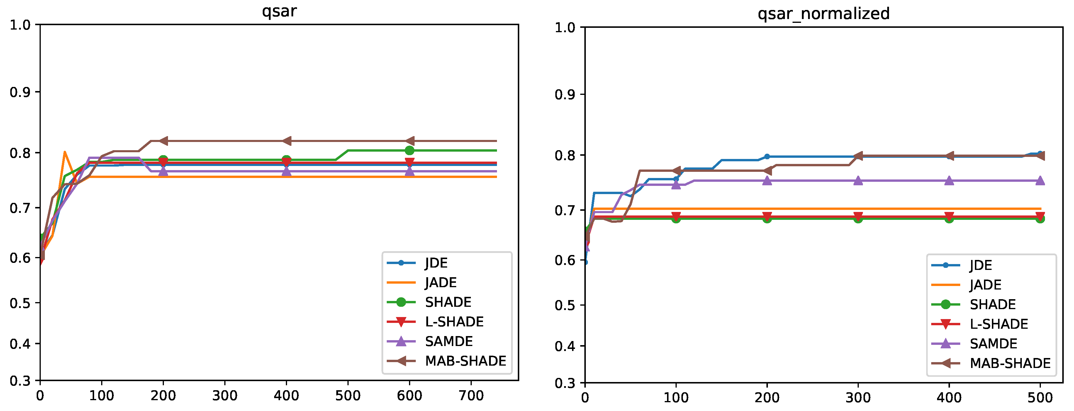
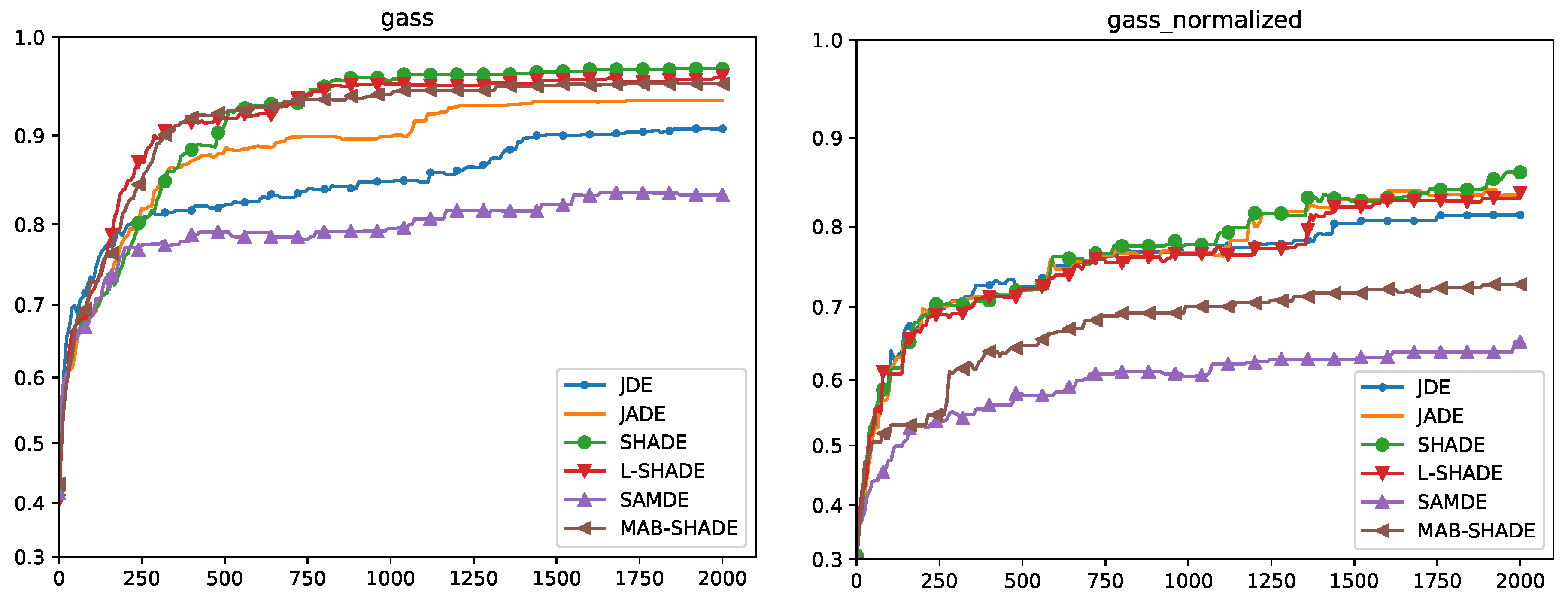
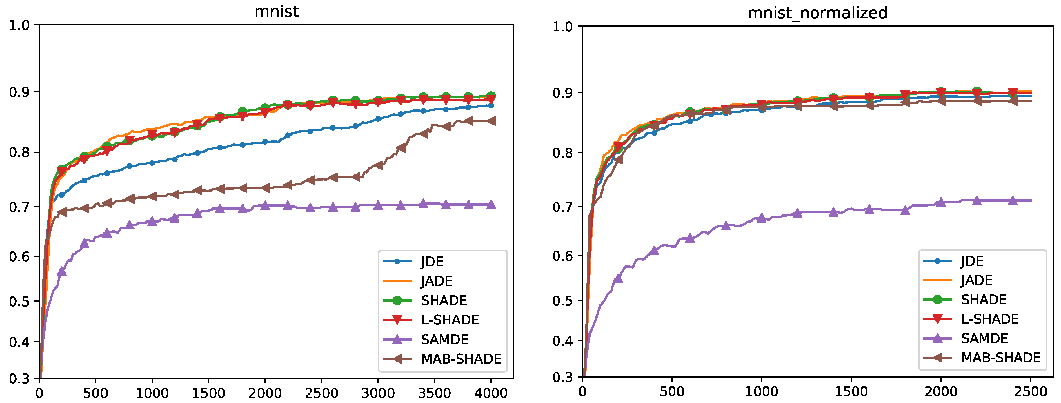
The first analysis has been made on the convergence graphics, where for each dataset the data of accuracy has been plotted during the generations. For each dataset and for each self-adaptive method, the data of the method which obtained the highest accuracy have been displayed in Figure 1, Figure 2, Figure 3 and Figure 4.

From the plots, it is possible to see that, excluding the cases where the differences are not significant, MAB-ShaDE works well on smaller datasets (MAGIC and QSAR), whereas ShaDE is the best method for larger datasets.

5.4. Convergence Analysis

In this subsection, we discuss the convergence across all DE used and analyzed in this paper on the datasets discussed before. On the MAGIC dataset, SHADE and L-SHADE converge in around 1750 generations, whereas the proposed MAB-SHADE requires only 250 generations to achieve a solution with a comparable quality. Other methods were able to discover lower quality solutions only. Regarding the other binary classification problem, QSAR, MAB-SHADE converges faster than all the other methods in less than 200 generations, while simultaneously obtaining a higher quality solution.

On the GASS multi-class problem, MAB-SHADE follow the same convergence path of L-SHADE, whereas SHADE has a slow convergence, but the quality of result reached by SHADE is slightly better, conversely, the other methods do not reach a satisfactory solution.

On the image classification problem MNIST, SHADE and L-SHADE resulted the best algorithms in terms of the solution quality and the time of convergence, whereas the other methods did not obtain comparable solutions in terms of quality; noticeably, MAB-SHADE did not get stuck, but it is likely that it requires more generations to converge to a solution.

We also performed the same tests with normalized versions of the datasets, finding susceptible differences with the previous results.

On MAGIC all the methods converged to the same solution, whereas on QSAR the best solution was reached by MAB-SHADE and jDE. Regarding GASS, no analyzed method reached a solution comparable in terms of quality to the solutions found on the corresponding original dataset. Finally, on MNIST all the methods, except SAMDE, reached good solutions, which are, however, below the solutions found with SHADE on the non normalized datasets.

Generally speaking, the best DE method is SHADE for the multi-class problems and MAB-SHADE for binary classification. Anyway, the convergence curves of SHADE are close to those of MAB-SHADE in the latter kind of problems.

Finally, it is worth to notice that MAB-SHADE performed systematically better than its direct competitor SAMDE without requiring to choose a particular mutation strategy.

Quade Weighted Rank

As we have different results for different datasets, we applied the Quade test [48] in order to obtain a global ranking which takes into account the differences among the datasets.

The Quade test considers that some datasets could be more difficult to deal with (i.e., the differences in accuracy of the various algorithms are larger). In this way, the rankings computed on each dataset are scaled depending on the differences observed in the algorithms’ performances [48].

With reference to

Table 3. Top 20 Quade ranking for parameter configurations.

Rank	Method	Mutation	Crossoverb	r	s	QUADE Rank
1	SHADE	curr_p_best	interm	high	1	$\frac{B}{2R}$	2713
2	SHADE	curr_p_best	interm	high	2	$\frac{B}{4R}$	3011
3	L–SHADE	curr_p_best	interm	high	4	$\frac{B}{R}$	3199
4	SHADE	curr_p_best	interm	mid	4	$\frac{B}{4R}$	3291
5	SHADE	curr_p_best	interm	high	1	$\frac{B}{R}$	3330
6	SHADE	curr_p_best	interm	low	2	$\frac{B}{2R}$	3365
7	JDE	degl	bin	high	2	$\frac{B}{4R}$	3721
8	JADE	curr_p_best	interm	high	2	$\frac{B}{R}$	3808
9	JDE	curr_p_best	interm	high	1	$\frac{B}{R}$	3838
10	L–SHADE	curr_p_best	interm	high	1	$\frac{B}{2R}$	3872
11	L–SHADE	curr_p_best	bin	high	2	$\frac{B}{2R}$	3897
12	SHADE	curr_p_best	interm	high	4	$\frac{B}{4R}$	3928
13	SHADE	rand/1	interm	high	1	$\frac{B}{2R}$	4108
14	L–SHADE	curr_p_best	interm	high	2	$\frac{B}{R}$	4160
15	MAB–SHADE	None	bin	high	1	$\frac{B}{R}$	4194
16	JADE	curr_p_best	interm	mid	4	$\frac{B}{2R}$	4267
17	SHADE	curr_p_best	interm	high	1	$\frac{B}{4R}$	4355
18	SHADE	curr_p_best	bin	high	2	$\frac{B}{2R}$	4356
19	JADE	degl	bin	low	2	$\frac{B}{4R}$	4423
20	JDE	degl	bin	high	4	$\frac{B}{2R}$	4513

, for each algorithm combination, the weighted ranking values are shown in the last column Quade rank.

These values are computed as follows.

Given the 756 parameter configurations we obtained by varying the values for each dimensions as shown in Table 1, we memorized in $v_{ij}$ the average accuracy value obtained by the configuration in the row i on the dataset in the column j. The ranks $r_{ij}$ of these values are computed for each dataset. Ranks are also assigned to the datasets according to the sample range of accuracy values obtained on it. The sample range within data set j is the difference between the largest and the smallest accuracy $v_{ij}$ within that data set. Let $Q_j$ be the rank assigned to the j-th dataset with respect to these values. Then, the Quade weighted rank is obtained ordering the parameters configuration with respect to $S_j={\sum }_i{r}_{ij}{Q}_j$.

In Table 3, the top 20 among the 756 configurations tested are shown. We can see that SHADE, curr_p_best, interm, and $b=high$ are the best choices.

5.5. Execution Times

The execution time of DENN changes with respect to the number of features and the size of batch. Therefore, in

Table 4. Average execution times.

Dataset	b = Low	b = Mid	b = High
MAGIC	$0.571$	$0.593$	$0.612$
MAGIC-N	$0.583$	$0.591$	$0.625$
QSAR	$0.760$	$0.776$	$0.783$
QSAR-N	$0.748$	$0.752$	$0.779$
GASS	$7.740$	$9.676$	$10.819$
GASS-N	$7.751$	$9.617$	$10.797$
MNIST	$133.748$	$154.731$	$194.948$
MNIST-N	$132.615$	$155.842$	$191.055$

, we show the average execution time in seconds of DENN in each datasets and for each level of b. Note that the execution time is not sensitively affected by the normalization of the datasets.

In Table 4, the worst case required approximately three minutes for the computation of the solution also thanks to a strong parallelization of the computation. Note that this point is a plus of the evolutionary approach: in the case of an iterative method like backpropagation it would have been impossible. Therefore, we can conclude that the time to reach the solution is reasonable and the approach is feasible, even if it is slower when compared to gradient-based methods.

5.6. Comparison with Backpropagation

In this section, we compared our method to the Backpropagation (BPG) algorithm, using two optimizer: the Stochastic Gradient Descendent (SGD) and the more powerful Adam. The experiments were performed on the same datasets MAGIC, QSAR, GASS, and MNIST, using both the original and the normalized versions.

The results are reported in

Table 5. Comparison BPG - DENN.

Dataset	BPG+SGD	BPG+ADAM	DENN
MAGIC	$73.0\%$	$71.9\%$	$76.6\%$
MAGIC-N	$77.0\%$	$78.2\%$	$78.8\%$
QSAR	$78.9\%$	$72.5\%$	$79.9\%$
QSAR-N	$80.6\%$	$80.6\%$	$81.4\%$
GASS	$73.9\%$	$68.9\%$	$86.2\%$
GASS-N	$89.8\%$	$94.6\%$	$96.8\%$
MNIST	$90.3\%$	$90.7\%$	$89.4\%$
MNIST-N	$90.1\%$	$90.5\%$	$90.4\%$

, where for each dataset we compare the classification accuracy obtained by NNs trained with BPG (using both optimizers) to the accuracy obtained by our method (DENN). As it can be seen in the results, in such a scenario our method shows better performances or, in some cases, comparable to the competitors. More specifically, DENN obtained higher accuracy if compared to SGD on all classification problems, while ADAM performed better only on MNIST.

The difference between MNIST and other datasets is about their features. In MNIST, the features are just quantitative; whereas, in the other ones, some data has a quantitative nature and other data are qualitative.

Generally, all the algorithms work better on normalized datasets, except that in MNIST, where data have are already a high degree of homogeneity. On the other hand, in GASS the effect of using normalized datasets is much greater for all the algorithms.

Note that our method can be useful in MLP networks trained for problems on which traditional algorithms can hardly achieve satisfying performances or need larger networks to achieve the same results.

6. Conclusions and Future Works

In this paper the DENN framework, a learning algorithm for Neural Networks based on Self-Adaptive Differential Evolution, is presented. Experiments show that the framework is able to solve classification problems, reaching satisfying levels of accuracy even in case of large datasets. The use of batch systems allows the application of DE to new untested domains. Indeed, it is worth noticing that the size of the problems handled in this work is significantly larger than those tested in other works available in literature.

Furthermore, the per-layer mutation and crossover strategies introduced in this work perform better than the traditional DE used in previous works. From the experiments we found the following:

• the configuration of the Self-Adaptive ShaDE with curr_p_best and the new interm crossover performs better than other settings,
• the slow change of batches allows to reach better results, and
• the MAB-ShaDE algorithm reduces the number of parameters at the cost of slightly worse solutions.

The results obtained with DENN are almost always better than those obtained with backpropagation. Moreover DENN appears to be robust than its competitor with respect to the normalization.

Future research will investigate the possibility of using DENN as optimizer for other Neural Network structures, including Convolutional Neural Networks, Recurrent Neural Networks, and Neural Turing Machines. Another scenario could be the application of Evolutionary Algorithms to those problems and domains where gradient-based optimizers do not perform as well as in supervised learning. A first direction will be the application of DENN in the Reinforcement Learning context, where a NN approximates the Value-Action Function (or Q Function) for agents in a nonlinear and complex environment.

References

1. Cireşan, D.C.; Meier, U.; Gambardella, L.M.; Schmidhuber, J. Deep, big, simple neural nets for handwritten digit recognition. Neural Comput. 2010, 22, 3207–3220. [Google Scholar] [CrossRef] [PubMed] [Green Version]
2. Goodfellow, I.; Pouget-Abadie, J.; Mirza, M.; Xu, B.; Warde-Farley, D.; Ozair, S.; Courville, A.; Bengio, Y. Generative adversarial nets. In Advances in Neural Information Processing Systems; MIT: Cambridge, MA, USA, 2014; pp. 2672–2680. [Google Scholar]
3. Santucci, V.; Spina, S.; Milani, A.; Biondi, G.; Di Bari, G. Detecting hate speech for Italian language in social media. In Proceedings of the EVALITA 2018, co-located with the Fifth Italian Conference on Computational Linguistics (CLiC-it 2018), Turin, Italy, 12–13 December 2018; Volume 2263. [Google Scholar]
4. Graves, A.; Jaitly, N.; Mohamed, A.R. Hybrid speech recognition with deep bidirectional LSTM. In Proceedings of the 2013 IEEE workshop on automatic speech recognition and understanding, Olomouc, Czech Republic, 8–12 December 2013; pp. 273–278. [Google Scholar]
5. Biondi, G.; Franzoni, V.; Poggioni, V. A deep learning semantic approach to emotion recognition using the IBM watson bluemix alchemy language. In Lecture Notes in Computer Science; Springer: Cham, Switzerland, 2017; pp. 719–729. [Google Scholar]
6. Krizhevsky, A.; Sutskever, I.; Hinton, G.E. Imagenet classification with deep convolutional neural networks. In Advances in Neural Information Processing Systems; MIT: Cambridge, MA, USA, 2012; pp. 1097–1105. [Google Scholar]
7. Graves, A.; Wayne, G.; Danihelka, I. Neural turing machines. arXiv 2014, arXiv:1410.5401. [Google Scholar]
8. Kurach, K.; Andrychowicz, M.; Sutskever, I. Neural Random-Access Machines. arXiv 2015, arXiv:abs/1511.06392. [Google Scholar]
9. Hinton, G.; Deng, L.; Yu, D.; Dahl, G.; Mohamed, A.R.; Jaitly, N.; Senior, A.; Vanhoucke, V.; Nguyen, P.; Kingsbury, B.; et al. Deep Neural Networks for Acoustic Modeling in Speech Recognition: The Shared Views of Four Research Groups. IEEE Signal Process. Mag. 2012, 29, 82–97. [Google Scholar] [CrossRef]
10. Krizhevsky, A.; Sutskever, I.; Hinton, G.E. ImageNet Classification with Deep Convolutional Neural Networks. In Advances in Neural Information Processing Systems 25; Pereira, F., Burges, C.J.C., Bottou, L., Weinberger, K.Q., Eds.; Curran Associates, Inc.: Dutchess County, NY, USA, 2012; pp. 1097–1105. [Google Scholar]
11. Bengio, Y.; Goodfellow, I.J.; Courville, A. Deep learning. Nature 2015, 521, 436–444. [Google Scholar]
12. Baioletti, M.; Di Bari, G.; Poggioni, V.; Tracolli, M. Can Differential Evolution Be an Efficient Engine to Optimize Neural Networks? In Machine Learning, Optimization, and Big Data; Springer International Publishing: Cham, Switzerland, 2018; pp. 401–413. [Google Scholar]
13. Donate, J.P.; Li, X.; Sánchez, G.G.; de Miguel, A.S. Time series forecasting by evolving artificial neural networks with genetic algorithms, differential evolution and estimation of distribution algorithm. Neural Comput. Appl. 2013, 22, 11–20. [Google Scholar] [CrossRef]
14. Wang, L.; Zeng, Y.; Chen, T. Back propagation neural network with adaptive differential evolution algorithm for time series forecasting. Expert Syst. Appl. 2015, 42, 855–863. [Google Scholar] [CrossRef]
15. Morse, G.; Stanley, K.O. Simple Evolutionary Optimization Can Rival Stochastic Gradient Descent in Neural Networks. In Proceedings of the Genetic and Evolutionary Computation Conference (GECCO), Denver, CO, USA, 20–24 July 2016; ACM: New York, NY, USA, 2016; pp. 477–484. [Google Scholar]
16. Miikkulainen, R. Neuroevolution. In Encyclopedia of Machine Learning; Springer: Boston, MA, USA, 2010; pp. 716–720. [Google Scholar]
17. Floreano, D.; Dürr, P.; Mattiussi, C. Neuroevolution: From architectures to learning. Evol. Intell. 2008, 1, 47–62. [Google Scholar] [CrossRef]
18. Rumelhart, D.E.; Hinton, G.E.; Williams, R.J. Learning representations by back-propagating errors. Nature 1986, 323, 533. [Google Scholar] [CrossRef]
19. Eltaeib, T.; Mahmood, A. Differential Evolution: A Survey and Analysis. Appl. Sci. 2018, 8, 1945. [Google Scholar] [CrossRef] [Green Version]
20. Kitayama, S.; Arakawa, M.; Yamazaki, K. Differential evolution as the global optimization technique and its application to structural optimization. Appl. Soft Comput. 2011, 11, 3792–3803. [Google Scholar] [CrossRef] [Green Version]
21. Zou, D.; Wu, J.; Gao, L.; Li, S. A modified differential evolution algorithm for unconstrained optimization problems. Neurocomputing 2013, 120, 469–481. [Google Scholar] [CrossRef]
22. Yao, X. Evolving artificial neural networks. Proc. IEEE 1999, 87, 1423–1447. [Google Scholar]
23. Such, F.P.; Madhavan, V.; Conti, E.; Lehman, J.; Stanley, K.O.; Clune, J. Deep Neuroevolution: Genetic Algorithms Are a Competitive Alternative for Training Deep Neural Networks for Reinforcement Learning. arXiv 2017, arXiv:1712.06567. [Google Scholar]
24. Vesterstrom, J.; Thomsen, R. A comparative study of differential evolution, particle swarm optimization, and evolutionary algorithms on numerical benchmark problems. In Proceedings of the 2004 Congress on Evolutionary Computation (IEEE Cat. No.04TH8753), Portland, OR, USA, 19–23 June 2004; Volume 2, pp. 1980–1987. [Google Scholar]
25. Price, K.; Storn, R.M.; Lampinen, J.A. Differential Evolution: A Practical Approach to Global Optimization; Springer Science & Business Media: Berlin/Heidelberg, Germany, 2006. [Google Scholar]
26. Zhang, X.; Xue, Y.; Lu, X.; Jia, S. Differential-Evolution-Based Coevolution Ant Colony Optimization Algorithm for Bayesian Network Structure Learning. Algorithms 2018, 11, 188. [Google Scholar] [CrossRef] [Green Version]
27. Gämperle, R.; Müller, S.D.; Koumoutsakos, P. A parameter study for differential evolution. Adv. Intell. Syst. Fuzzy Syst. Evol. Comput. 2002, 10, 293–298. [Google Scholar]
28. Santucci, V. Linear Ordering Optimization with a Combinatorial Differential Evolution. In Proceedings of the IEEE International Conference on Systems, Man, and Cybernetics, SMC 2015, Kowloon, China, 9–12 October 2015; IEEE Press: Piscataway, NJ, USA, 2016; pp. 2135–2140. [Google Scholar] [CrossRef]
29. Santucci, V. A differential evolution algorithm for the permutation flowshop scheduling problem with total flow time criterion. In Lecture Notes in Computer Science; LNCS 8672; Springer: Berlin/Heidelberg, Germany, 2016; pp. 161–170. ISBN 03029743. [Google Scholar]
30. Piotrowski, A.P. Differential Evolution algorithms applied to Neural Network training suffer from stagnation. Appl. Soft Comput. 2014, 21, 382–406. [Google Scholar] [CrossRef]
31. Chen, W.; Wang, Y.; Yuan, Y.; Wang, Q. Combinatorial Multi-armed Bandit and Its Extension to Probabilistically Triggered Arms. J. Mach. Learn. Res. 2016, 17, 1746–1778. [Google Scholar]
32. Das, S.; Mullick, S.S.; Suganthan, P. Recent advances in differential evolution—An updated survey. Swarm Evol. Comput. 2016, 27, 1–30. [Google Scholar] [CrossRef]
33. Storn, R.; Price, K. Differential Evolution—A Simple and Efficient Heuristic for global Optimization over Continuous Spaces. J. Glob. Optim. 1997, 11, 341–359. [Google Scholar] [CrossRef]
34. Tanabe, R.; Fukunaga, A. Success-History Based Parameter Adaptation for Differential Evolution. In Proceedings of the IEEE Congress on Evolutionary Computation, Cancun, Mexico, 20–23 June 2013. [Google Scholar]
35. Das, S.; Abraham, A.; Chakraborty, U.K.; Konar, A. Differential Evolution Using a Neighborhood-Based Mutation Operator. IEEE Trans. Evol. Comput. 2009, 13, 526–553. [Google Scholar] [CrossRef] [Green Version]
36. Brest, J.; Boskovic, B.; Mernik, M.; Zumer, V. Self-Adapting Control Parameters in Differential Evolution: A Comparative Study on Numerical Benchmark Problems. IEEE Trans. Evol. Comput. 2006, 10, 646–657. [Google Scholar] [CrossRef]
37. Peng, F.; Tang, K.; Chen, G.; Yao, X. Multi-start JADE with knowledge transfer for numerical optimization. In Proceedings of the 2009 IEEE Congress on Evolutionary Computation, Trondheim, Norway, 18–21 May 2009; pp. 1889–1895. [Google Scholar]
38. Tanabe, R.; Fukunaga, A.S. Improving the Search Performance of SHADE Using Linear Population Size Reduction. In Proceedings of the 2014 IEEE Congress on Evolutionary Computation (CEC), Beijing, China, 6–11 July 2014. [Google Scholar]
39. Pedrosa Silva, R.; Lopes, R.; Guimarães, F. Self-adaptive mutation in the Differential Evolution: Self- * search. In Proceedings of the Genetic and Evolutionary Computation Conference, GECCO’11, Dublin, Ireland, 12–16 July 2011; pp. 1939–1946. [Google Scholar]
40. Ilonen, J.; Kamarainen, J.K.; Lampinen, J. Differential evolution training algorithm for feedforward neural networks. Neural Process. Lett. 2003, 17, 93–105. [Google Scholar] [CrossRef]
41. Masters, T.; Land, W. A new training algorithm for the general regression neural network. In Proceedings of the 1997 IEEE International Conference on Systems, Man, and Cybernetics, Orlando, FL, USA, 12–15 October 1997; Volume 3, pp. 1990–1994. [Google Scholar]
42. Schraudolph, N.N.; Belew, R.K. Dynamic parameter encoding for genetic algorithms. Mach. Learn. 1992, 9, 9–21. [Google Scholar] [CrossRef] [Green Version]
43. Mattiussi, C.; Dürr, P.; Floreano, D. Center of Mass Encoding: A Self-adaptive Representation with Adjustable Redundancy for Real-valued Parameters. In Proceedings of the Genetic and Evolutionary Computation Conference, London, UK, 7–11 July 2007; ACM: New York, NY, USA, 2007; pp. 1304–1311. [Google Scholar]
44. Mancini, L.; Milani, A.; Poggioni, V.; Chiancone, A. Self regulating mechanisms for network immunization. AI Commun. 2016, 29, 301–317. [Google Scholar] [CrossRef]
45. Franzoni, V.; Chiancone, A. A Multistrain Bacterial Diffusion Model for Link Prediction. Int. J. Pattern Recognit. Artif. Intell. 2017, 31. [Google Scholar] [CrossRef]
46. Heidrich-Meisner, V.; Igel, C. Neuroevolution strategies for episodic reinforcement learning. J. Algorithms 2009, 64, 152–168. [Google Scholar] [CrossRef]
47. Leema, N.; Nehemiah, H.K.; Kannan, A. Neural network classifier optimization using Differential Evolution with Global Information and Back Propagation algorithm for clinical datasets. Appl. Soft Comput. 2016, 49, 834–844. [Google Scholar] [CrossRef]
48. Quade, D. Using weighted rankings in the analysis of complete blocks with additive block effects. J. Am. Stat. Assoc. 1979, 74, 680–683. [Google Scholar] [CrossRef]
Figure 1. Plots of convergences on MAGIC and MAGIC normalized datasets.
Mathematics 08 00069 g001
Figure 2. Plots of convergences on QSAR and QSAR normalized datasets.
Mathematics 08 00069 g002
Figure 3. Plots of convergences on GASS and GASS normalized datasets.
Mathematics 08 00069 g003
Figure 4. Plots of convergences on MNIST and MNIST normalized datasets.
Mathematics 08 00069 g004