Differential Evolution for Neural Networks Optimization


Abstract
1. Introduction
2. Background
2.1. Differential Evolution
2.1.1. Self-Adaptive Differential Evolution
2.1.2. Self-Adaptive Mutation
2.2. Neuroevolution
3. Related Works
4. The DENN Algorithm
| Algorithm 1: The algorithm DENN |
 |
4.1. Fitness Function
4.2. The Interm Crossover
4.3. The MAB-ShaDE Mutation Method
5. Experiments
5.1. Datasets
- MAGIC Gamma telescope:dataset with 19,020 records, 10 features, and two classes.
- QSAR biodegradation: dataset with 1055 records, 41 features, and two classes.
- GASS Sensor Array Drift: dataset with 13,910 records, 128 features, and six classes.
- MNIST: dataset with 70,000 records, 784 features, and 10 classes.
5.2. System Parameters
- the auto-adaptive variant of DE (simply called Method),
- the Mutation operator,
- the Crossover operator,
- the number s of generations of a sub-epoch,
- the batch/window size b, and
- the ratio r between the batch size and the number of records changed in the window at each sub-epoch.
5.3. Algorithm Combination Analysis
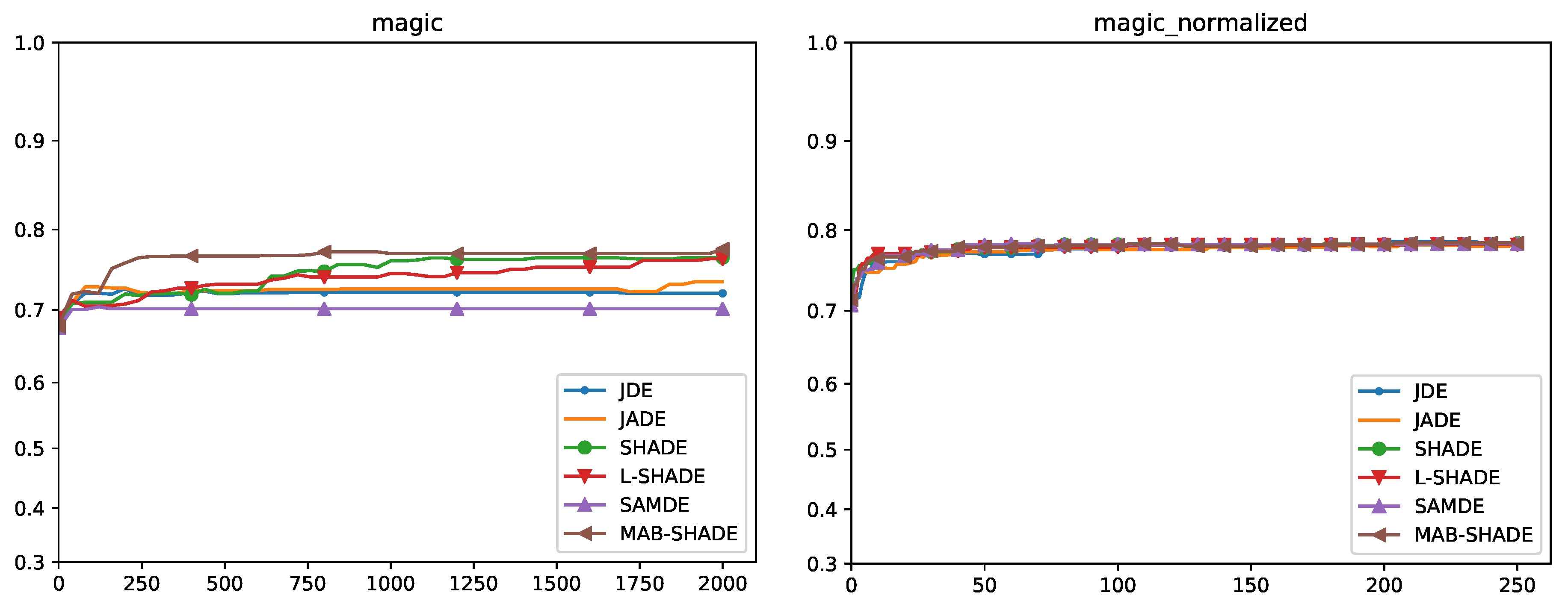
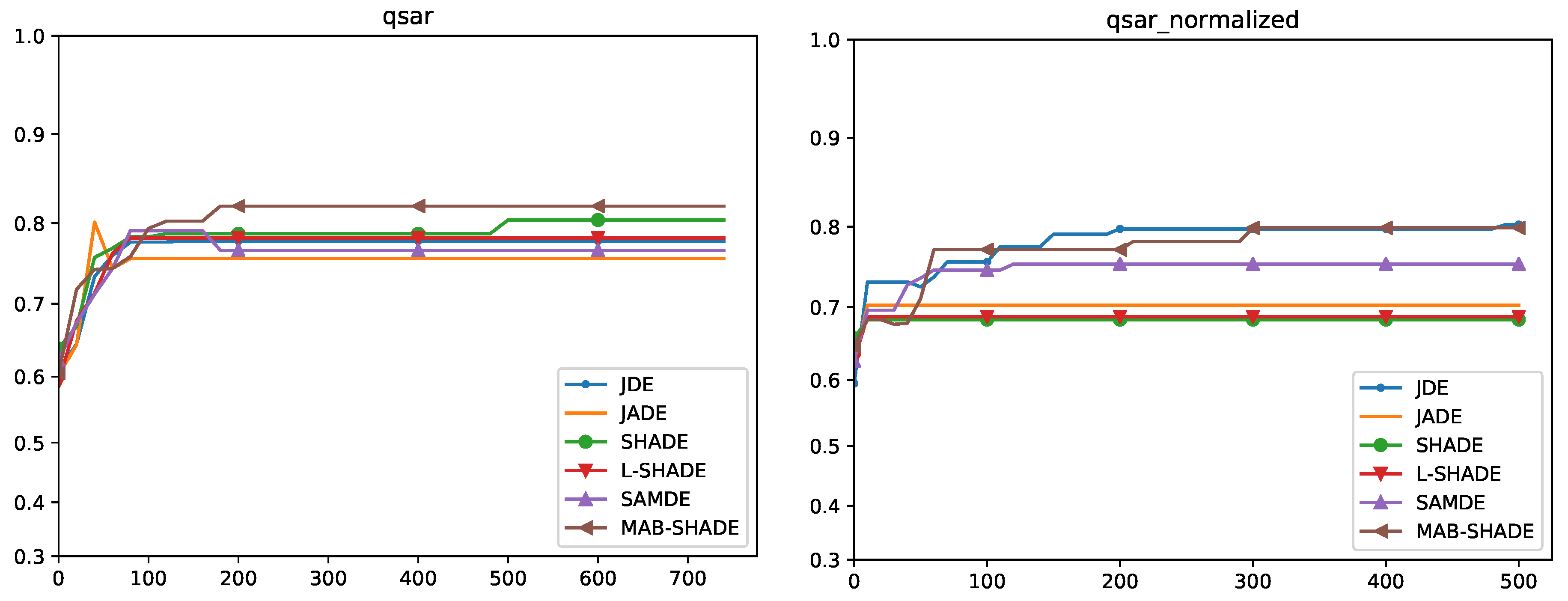
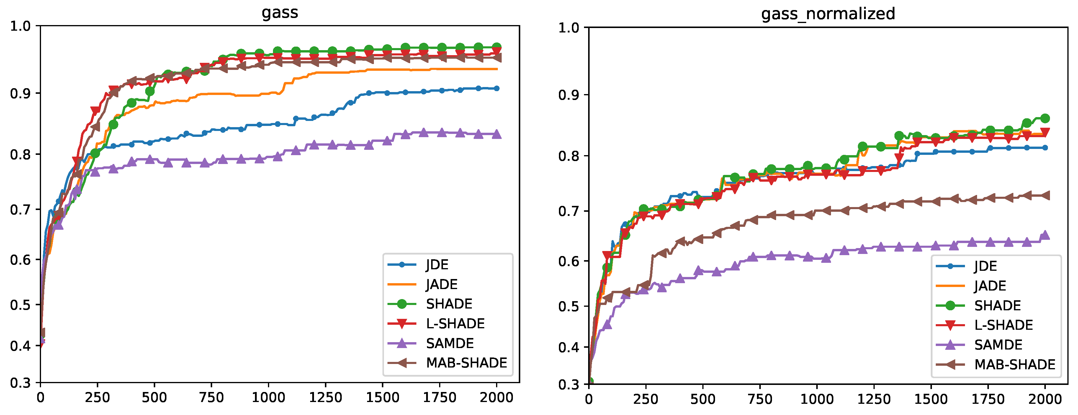
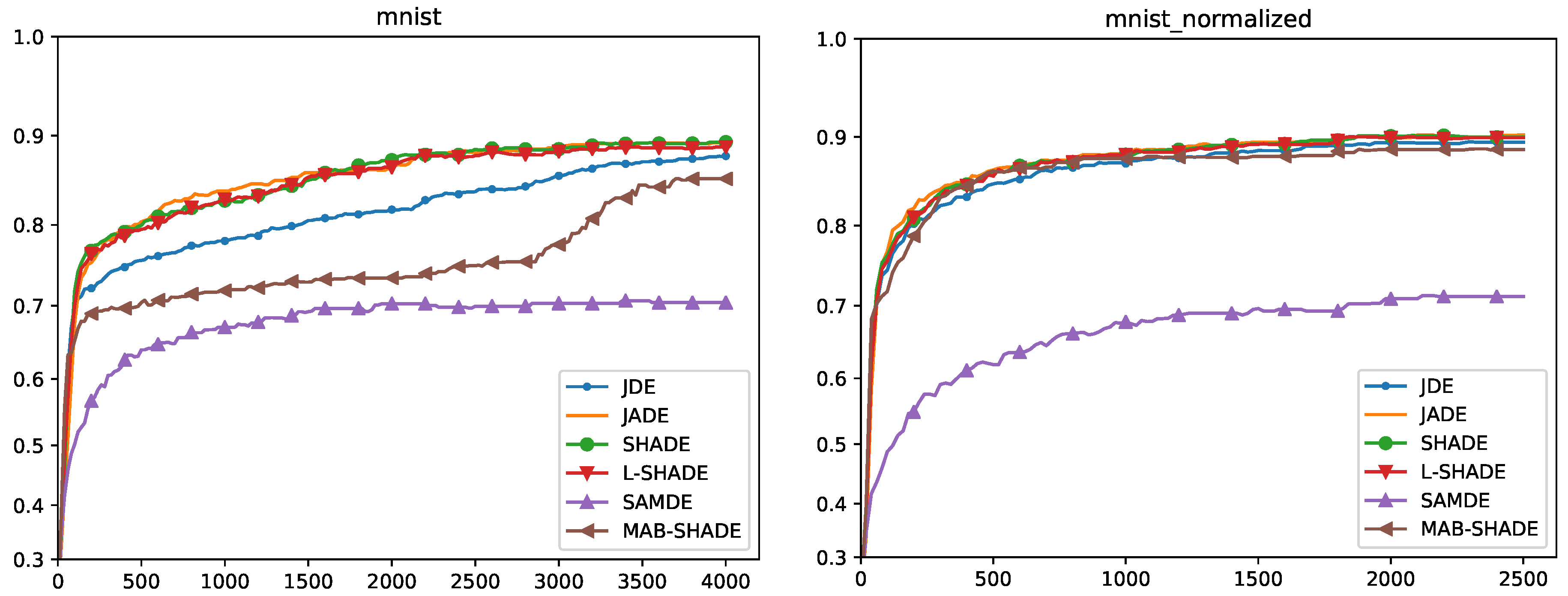
5.4. Convergence Analysis
Quade Weighted Rank
5.5. Execution Times
5.6. Comparison with Backpropagation
6. Conclusions and Future Works
- the configuration of the Self-Adaptive ShaDE with curr_p_best and the new interm crossover performs better than other settings,
- the slow change of batches allows to reach better results, and
- the MAB-ShaDE algorithm reduces the number of parameters at the cost of slightly worse solutions.
Author Contributions
Funding
Conflicts of Interest
References
- Cireşan, D.C.; Meier, U.; Gambardella, L.M.; Schmidhuber, J. Deep, big, simple neural nets for handwritten digit recognition. Neural Comput. 2010, 22, 3207–3220. [Google Scholar] [CrossRef] [PubMed]
- Goodfellow, I.; Pouget-Abadie, J.; Mirza, M.; Xu, B.; Warde-Farley, D.; Ozair, S.; Courville, A.; Bengio, Y. Generative adversarial nets. In Advances in Neural Information Processing Systems; MIT: Cambridge, MA, USA, 2014; pp. 2672–2680. [Google Scholar]
- Santucci, V.; Spina, S.; Milani, A.; Biondi, G.; Di Bari, G. Detecting hate speech for Italian language in social media. In Proceedings of the EVALITA 2018, co-located with the Fifth Italian Conference on Computational Linguistics (CLiC-it 2018), Turin, Italy, 12–13 December 2018; Volume 2263. [Google Scholar]
- Graves, A.; Jaitly, N.; Mohamed, A.R. Hybrid speech recognition with deep bidirectional LSTM. In Proceedings of the 2013 IEEE workshop on automatic speech recognition and understanding, Olomouc, Czech Republic, 8–12 December 2013; pp. 273–278. [Google Scholar]
- Biondi, G.; Franzoni, V.; Poggioni, V. A deep learning semantic approach to emotion recognition using the IBM watson bluemix alchemy language. In Lecture Notes in Computer Science; Springer: Cham, Switzerland, 2017; pp. 719–729. [Google Scholar]
- Krizhevsky, A.; Sutskever, I.; Hinton, G.E. Imagenet classification with deep convolutional neural networks. In Advances in Neural Information Processing Systems; MIT: Cambridge, MA, USA, 2012; pp. 1097–1105. [Google Scholar]
- Graves, A.; Wayne, G.; Danihelka, I. Neural turing machines. arXiv 2014, arXiv:1410.5401. [Google Scholar]
- Kurach, K.; Andrychowicz, M.; Sutskever, I. Neural Random-Access Machines. arXiv 2015, arXiv:abs/1511.06392. [Google Scholar]
- Hinton, G.; Deng, L.; Yu, D.; Dahl, G.; Mohamed, A.R.; Jaitly, N.; Senior, A.; Vanhoucke, V.; Nguyen, P.; Kingsbury, B.; et al. Deep Neural Networks for Acoustic Modeling in Speech Recognition: The Shared Views of Four Research Groups. IEEE Signal Process. Mag. 2012, 29, 82–97. [Google Scholar] [CrossRef]
- Krizhevsky, A.; Sutskever, I.; Hinton, G.E. ImageNet Classification with Deep Convolutional Neural Networks. In Advances in Neural Information Processing Systems 25; Pereira, F., Burges, C.J.C., Bottou, L., Weinberger, K.Q., Eds.; Curran Associates, Inc.: Dutchess County, NY, USA, 2012; pp. 1097–1105. [Google Scholar]
- Bengio, Y.; Goodfellow, I.J.; Courville, A. Deep learning. Nature 2015, 521, 436–444. [Google Scholar]
- Baioletti, M.; Di Bari, G.; Poggioni, V.; Tracolli, M. Can Differential Evolution Be an Efficient Engine to Optimize Neural Networks? In Machine Learning, Optimization, and Big Data; Springer International Publishing: Cham, Switzerland, 2018; pp. 401–413. [Google Scholar]
- Donate, J.P.; Li, X.; Sánchez, G.G.; de Miguel, A.S. Time series forecasting by evolving artificial neural networks with genetic algorithms, differential evolution and estimation of distribution algorithm. Neural Comput. Appl. 2013, 22, 11–20. [Google Scholar] [CrossRef]
- Wang, L.; Zeng, Y.; Chen, T. Back propagation neural network with adaptive differential evolution algorithm for time series forecasting. Expert Syst. Appl. 2015, 42, 855–863. [Google Scholar] [CrossRef]
- Morse, G.; Stanley, K.O. Simple Evolutionary Optimization Can Rival Stochastic Gradient Descent in Neural Networks. In Proceedings of the Genetic and Evolutionary Computation Conference (GECCO), Denver, CO, USA, 20–24 July 2016; ACM: New York, NY, USA, 2016; pp. 477–484. [Google Scholar]
- Miikkulainen, R. Neuroevolution. In Encyclopedia of Machine Learning; Springer: Boston, MA, USA, 2010; pp. 716–720. [Google Scholar]
- Floreano, D.; Dürr, P.; Mattiussi, C. Neuroevolution: From architectures to learning. Evol. Intell. 2008, 1, 47–62. [Google Scholar] [CrossRef]
- Rumelhart, D.E.; Hinton, G.E.; Williams, R.J. Learning representations by back-propagating errors. Nature 1986, 323, 533. [Google Scholar] [CrossRef]
- Eltaeib, T.; Mahmood, A. Differential Evolution: A Survey and Analysis. Appl. Sci. 2018, 8, 1945. [Google Scholar] [CrossRef]
- Kitayama, S.; Arakawa, M.; Yamazaki, K. Differential evolution as the global optimization technique and its application to structural optimization. Appl. Soft Comput. 2011, 11, 3792–3803. [Google Scholar] [CrossRef]
- Zou, D.; Wu, J.; Gao, L.; Li, S. A modified differential evolution algorithm for unconstrained optimization problems. Neurocomputing 2013, 120, 469–481. [Google Scholar] [CrossRef]
- Yao, X. Evolving artificial neural networks. Proc. IEEE 1999, 87, 1423–1447. [Google Scholar]
- Such, F.P.; Madhavan, V.; Conti, E.; Lehman, J.; Stanley, K.O.; Clune, J. Deep Neuroevolution: Genetic Algorithms Are a Competitive Alternative for Training Deep Neural Networks for Reinforcement Learning. arXiv 2017, arXiv:1712.06567. [Google Scholar]
- Vesterstrom, J.; Thomsen, R. A comparative study of differential evolution, particle swarm optimization, and evolutionary algorithms on numerical benchmark problems. In Proceedings of the 2004 Congress on Evolutionary Computation (IEEE Cat. No.04TH8753), Portland, OR, USA, 19–23 June 2004; Volume 2, pp. 1980–1987. [Google Scholar]
- Price, K.; Storn, R.M.; Lampinen, J.A. Differential Evolution: A Practical Approach to Global Optimization; Springer Science & Business Media: Berlin/Heidelberg, Germany, 2006. [Google Scholar]
- Zhang, X.; Xue, Y.; Lu, X.; Jia, S. Differential-Evolution-Based Coevolution Ant Colony Optimization Algorithm for Bayesian Network Structure Learning. Algorithms 2018, 11, 188. [Google Scholar] [CrossRef]
- Gämperle, R.; Müller, S.D.; Koumoutsakos, P. A parameter study for differential evolution. Adv. Intell. Syst. Fuzzy Syst. Evol. Comput. 2002, 10, 293–298. [Google Scholar]
- Santucci, V. Linear Ordering Optimization with a Combinatorial Differential Evolution. In Proceedings of the IEEE International Conference on Systems, Man, and Cybernetics, SMC 2015, Kowloon, China, 9–12 October 2015; IEEE Press: Piscataway, NJ, USA, 2016; pp. 2135–2140. [Google Scholar] [CrossRef]
- Santucci, V. A differential evolution algorithm for the permutation flowshop scheduling problem with total flow time criterion. In Lecture Notes in Computer Science; LNCS 8672; Springer: Berlin/Heidelberg, Germany, 2016; pp. 161–170. ISBN 03029743. [Google Scholar]
- Piotrowski, A.P. Differential Evolution algorithms applied to Neural Network training suffer from stagnation. Appl. Soft Comput. 2014, 21, 382–406. [Google Scholar] [CrossRef]
- Chen, W.; Wang, Y.; Yuan, Y.; Wang, Q. Combinatorial Multi-armed Bandit and Its Extension to Probabilistically Triggered Arms. J. Mach. Learn. Res. 2016, 17, 1746–1778. [Google Scholar]
- Das, S.; Mullick, S.S.; Suganthan, P. Recent advances in differential evolution—An updated survey. Swarm Evol. Comput. 2016, 27, 1–30. [Google Scholar] [CrossRef]
- Storn, R.; Price, K. Differential Evolution—A Simple and Efficient Heuristic for global Optimization over Continuous Spaces. J. Glob. Optim. 1997, 11, 341–359. [Google Scholar] [CrossRef]
- Tanabe, R.; Fukunaga, A. Success-History Based Parameter Adaptation for Differential Evolution. In Proceedings of the IEEE Congress on Evolutionary Computation, Cancun, Mexico, 20–23 June 2013. [Google Scholar]
- Das, S.; Abraham, A.; Chakraborty, U.K.; Konar, A. Differential Evolution Using a Neighborhood-Based Mutation Operator. IEEE Trans. Evol. Comput. 2009, 13, 526–553. [Google Scholar] [CrossRef]
- Brest, J.; Boskovic, B.; Mernik, M.; Zumer, V. Self-Adapting Control Parameters in Differential Evolution: A Comparative Study on Numerical Benchmark Problems. IEEE Trans. Evol. Comput. 2006, 10, 646–657. [Google Scholar] [CrossRef]
- Peng, F.; Tang, K.; Chen, G.; Yao, X. Multi-start JADE with knowledge transfer for numerical optimization. In Proceedings of the 2009 IEEE Congress on Evolutionary Computation, Trondheim, Norway, 18–21 May 2009; pp. 1889–1895. [Google Scholar]
- Tanabe, R.; Fukunaga, A.S. Improving the Search Performance of SHADE Using Linear Population Size Reduction. In Proceedings of the 2014 IEEE Congress on Evolutionary Computation (CEC), Beijing, China, 6–11 July 2014. [Google Scholar]
- Pedrosa Silva, R.; Lopes, R.; Guimarães, F. Self-adaptive mutation in the Differential Evolution: Self- * search. In Proceedings of the Genetic and Evolutionary Computation Conference, GECCO’11, Dublin, Ireland, 12–16 July 2011; pp. 1939–1946. [Google Scholar]
- Ilonen, J.; Kamarainen, J.K.; Lampinen, J. Differential evolution training algorithm for feedforward neural networks. Neural Process. Lett. 2003, 17, 93–105. [Google Scholar] [CrossRef]
- Masters, T.; Land, W. A new training algorithm for the general regression neural network. In Proceedings of the 1997 IEEE International Conference on Systems, Man, and Cybernetics, Orlando, FL, USA, 12–15 October 1997; Volume 3, pp. 1990–1994. [Google Scholar]
- Schraudolph, N.N.; Belew, R.K. Dynamic parameter encoding for genetic algorithms. Mach. Learn. 1992, 9, 9–21. [Google Scholar] [CrossRef]
- Mattiussi, C.; Dürr, P.; Floreano, D. Center of Mass Encoding: A Self-adaptive Representation with Adjustable Redundancy for Real-valued Parameters. In Proceedings of the Genetic and Evolutionary Computation Conference, London, UK, 7–11 July 2007; ACM: New York, NY, USA, 2007; pp. 1304–1311. [Google Scholar]
- Mancini, L.; Milani, A.; Poggioni, V.; Chiancone, A. Self regulating mechanisms for network immunization. AI Commun. 2016, 29, 301–317. [Google Scholar] [CrossRef]
- Franzoni, V.; Chiancone, A. A Multistrain Bacterial Diffusion Model for Link Prediction. Int. J. Pattern Recognit. Artif. Intell. 2017, 31. [Google Scholar] [CrossRef]
- Heidrich-Meisner, V.; Igel, C. Neuroevolution strategies for episodic reinforcement learning. J. Algorithms 2009, 64, 152–168. [Google Scholar] [CrossRef]
- Leema, N.; Nehemiah, H.K.; Kannan, A. Neural network classifier optimization using Differential Evolution with Global Information and Back Propagation algorithm for clinical datasets. Appl. Soft Comput. 2016, 49, 834–844. [Google Scholar] [CrossRef]
- Quade, D. Using weighted rankings in the analysis of complete blocks with additive block effects. J. Am. Stat. Assoc. 1979, 74, 680–683. [Google Scholar] [CrossRef]


| Parameter | Values |
|---|---|
| Method | JDE, JADE, ShaDE, L-ShaDE, MAB-ShaDE, SAMDE |
| Mutation | rand/1, curr_to_pbest, DEGL |
| Crossover | bin, interm |
| b | low, mid, high |
| r | 1, , |
| s | , , |
| Dataset | Low | Mid | High |
|---|---|---|---|
| MAGIC | 20 | 40 | 80 |
| QSAR | 10 | 20 | 40 |
| GASS | 20 | 40 | 80 |
| MNIST | 50 | 100 | 200 |
| Rank | Method | Mutation | Crossoverb | r | s | QUADE Rank | |
|---|---|---|---|---|---|---|---|
| 1 | SHADE | curr_p_best | interm | high | 1 | 2713 | |
| 2 | SHADE | curr_p_best | interm | high | 2 | 3011 | |
| 3 | L–SHADE | curr_p_best | interm | high | 4 | 3199 | |
| 4 | SHADE | curr_p_best | interm | mid | 4 | 3291 | |
| 5 | SHADE | curr_p_best | interm | high | 1 | 3330 | |
| 6 | SHADE | curr_p_best | interm | low | 2 | 3365 | |
| 7 | JDE | degl | bin | high | 2 | 3721 | |
| 8 | JADE | curr_p_best | interm | high | 2 | 3808 | |
| 9 | JDE | curr_p_best | interm | high | 1 | 3838 | |
| 10 | L–SHADE | curr_p_best | interm | high | 1 | 3872 | |
| 11 | L–SHADE | curr_p_best | bin | high | 2 | 3897 | |
| 12 | SHADE | curr_p_best | interm | high | 4 | 3928 | |
| 13 | SHADE | rand/1 | interm | high | 1 | 4108 | |
| 14 | L–SHADE | curr_p_best | interm | high | 2 | 4160 | |
| 15 | MAB–SHADE | None | bin | high | 1 | 4194 | |
| 16 | JADE | curr_p_best | interm | mid | 4 | 4267 | |
| 17 | SHADE | curr_p_best | interm | high | 1 | 4355 | |
| 18 | SHADE | curr_p_best | bin | high | 2 | 4356 | |
| 19 | JADE | degl | bin | low | 2 | 4423 | |
| 20 | JDE | degl | bin | high | 4 | 4513 |
| Dataset | b = Low | b = Mid | b = High |
|---|---|---|---|
| MAGIC | |||
| MAGIC-N | |||
| QSAR | |||
| QSAR-N | |||
| GASS | |||
| GASS-N | |||
| MNIST | |||
| MNIST-N |
| Dataset | BPG+SGD | BPG+ADAM | DENN |
|---|---|---|---|
| MAGIC | |||
| MAGIC-N | |||
| QSAR | |||
| QSAR-N | |||
| GASS | |||
| GASS-N | |||
| MNIST | |||
| MNIST-N |
© 2020 by the authors. Licensee MDPI, Basel, Switzerland. This article is an open access article distributed under the terms and conditions of the Creative Commons Attribution (CC BY) license (http://creativecommons.org/licenses/by/4.0/).
Share and Cite
Baioletti, M.; Di Bari, G.; Milani, A.; Poggioni, V. Differential Evolution for Neural Networks Optimization. Mathematics 2020, 8, 69. https://doi.org/10.3390/math8010069
Baioletti M, Di Bari G, Milani A, Poggioni V. Differential Evolution for Neural Networks Optimization. Mathematics. 2020; 8(1):69. https://doi.org/10.3390/math8010069
Chicago/Turabian StyleBaioletti, Marco, Gabriele Di Bari, Alfredo Milani, and Valentina Poggioni. 2020. "Differential Evolution for Neural Networks Optimization" Mathematics 8, no. 1: 69. https://doi.org/10.3390/math8010069
APA StyleBaioletti, M., Di Bari, G., Milani, A., & Poggioni, V. (2020). Differential Evolution for Neural Networks Optimization. Mathematics, 8(1), 69. https://doi.org/10.3390/math8010069