Article

A Novel Forward-Backward Algorithm for Solving Convex Minimization Problem in Hilbert Spaces

1
Research Center in Mathematics and Applied Mathematics, Department of Mathematics, Faculty of Science, Chiang Mai University, Chiang Mai 50200, Thailand
2
School of Science, University of Phayao, Phayao 56000, Thailand
*
Author to whom correspondence should be addressed.
Mathematics 2020, 8(1), 42; https://doi.org/10.3390/math8010042
Submission received: 12 December 2019 / Revised: 20 December 2019 / Accepted: 21 December 2019 / Published: 1 January 2020

Abstract

:
In this work, we aim to investigate the convex minimization problem of the sum of two objective functions. This optimization problem includes, in particular, image reconstruction and signal recovery. We then propose a new modified forward-backward splitting method without the assumption of the Lipschitz continuity of the gradient of functions by using the line search procedures. It is shown that the sequence generated by the proposed algorithm weakly converges to minimizers of the sum of two convex functions. We also provide some applications of the proposed method to compressed sensing in the frequency domain. The numerical reports show that our method has a better convergence behavior than other methods in terms of the number of iterations and CPU time. Moreover, the numerical results of the comparative analysis are also discussed to show the optimal choice of parameters in the line search.

1. Introduction

Let H be a real Hilbert space, and let f , g : H R { + } be proper, lower-semicontinuous, and convex functions. The convex minimization problem is modeled as follows:
min x H ( f ( x ) + g ( x ) ) .
Throughout this paper, assume that Problem (1) is nonempty, and the solution set is denoted by S * . We know that Problem (1) can be described by the fixed point equation, that is,
x = prox α g ( x α f ( x ) )
where α > 0 and prox g is the proximal operator of g defined by prox g = ( I d + g ) 1 where I d denotes the identity operator in H and g is the classical convex subdifferential of g. Using this fixed point equation, one can define the following iteration process:
x k + 1 = prox α k g backward step ( x k α k f ( x k ) ) forward step ,
where α k is a suitable stepsize. This algorithm is known as the forward-backward algorithm, and it includes, as special cases, the gradient method [1,2,3] and the proximal algorithm [4,5,6,7]. Recently, the construction of algorithms has become a crucial technique for solving some nonlinear and optimization problems (see also [8,9,10,11,12,13,14,15]).
In 2005, Combettes and Wajs [16] proposed the following algorithm, which is based on iteration (3) as follows:
Algorithm 1 ([16]). Given ϵ ( 0 , min { 1 , 1 α } ) and letting x 0 R N , for k 1 :
y k = x k α k f ( x k ) , x k + 1 = x k + λ k ( prox α k g y k x k ) ,
where α k [ ϵ , 2 α ϵ ] , λ k [ ϵ , 1 ] and α is the Lipschitz constant of the gradient of f .
It was proven that the sequence generated by (4) converges to minimizers of f + g . However, we note that the convergence of Algorithm 1 depends on the Lipschitz continuity of the gradient of f, which is not an easy task to find in general.
The Douglas–Rachford algorithm is another method that can be used to solve the problem (1). It is defined in the following manner:
Algorithm 2 ([16]). Fix ϵ ( 0 , 1 ) , γ > 0 and let x 0 R N . For k 1 , calculate
y k = prox γ g x k , x k + 1 = x k + λ k ( prox γ f ( 2 y k x k ) y k ) ,
where λ k [ ϵ , 2 ϵ ] .
It was shown that the sequence ( x k ) defined by (5) converges to minimizers of f + g . In this case, we see that the main drawback of Algorithm 2 is that it requires two proximity operators of convex functions f and g per iteration. This leads to a slow convergence speed of algorithms based on Algorithm 2. Please see Section 4 for its convergence.
Very recently, Cruz and Nghia [17] introduced the forward-backward algorithm by using the line search technique in the framework of Hilbert spaces. Assume that the following conditions are satisfied:
( A 1 ) f , g : H R { + } are two proper, l . s . c , convex functions where dom g dom f and dom g is nonempty, closed, and convex.
( A 2 ) f is Fréchet differentiable on an open set that contains dom g . The gradient f is uniformly continuous on bounded subsets of dom g . Moreover, it maps any bounded subset of dom g to a bounded set in H.
Linesearch 1.
Let σ > 0 , θ ( 0 , 1 ) and δ ( 0 , 1 2 ) .
Input. Given α = σ and J ( x , α ) : = prox α g ( x α f ( x ) ) with x dom g
  While α f ( J ( x , α ) ) f ( x ) > δ J ( x , α ) x
do α = θ α .
  End While
Output. α .
It was proven that Line Search 1 is well defined, i.e., this line search stops after finitely many steps. By this fact, Cruz and Nghia [17] also considered the following algorithm:
Algorithm 3.Fix σ > 0 , θ ( 0 , 1 ) and δ ( 0 , 1 2 ) , and let x 0 dom g . For k 1 , calculate:
x k + 1 = prox α k g ( x k α k f ( x k ) ) ,
with α k : = Line Search 1 ( x k , σ , θ , δ ) .
They showed that the sequence ( x k ) generated by Algorithm 3 involving the line search technique that eliminates the Lipschitz assumption on the gradient of f converges weakly to minimizers of f + g . It is observed that, to obtain its convergence, one has to find the stepsize α in each iteration. This can be costly and time consuming in computation.
Recently, there have been many works on modifying the forward-backward method for solving convex optimization problems (see, for example, [18,19,20,21,22,23]).
In variational theory, Tseng [24] introduced the following method for solving the variational inequality problem (VIP):
y k = P C ( x k λ F x k ) , x k + 1 = y k + λ ( F y k F x k ) ,
where P C is a metric projection from a Hilbert space onto the set C, F is a monotone and L-Lipschitz continuous mapping, and λ ( 0 , 1 / L ) . Then, the sequence generated by (6) weakly converges to a solution of VIP. This method is often called Tseng’s extragradient method and has received great attention by researchers due to its convergence speed (see, for example, [25,26,27,28]). Following this research direction, the main challenge is to design novel algorithms that can speed up the convergence rate compared to Algorithms 1–3.
In this paper, inspired by Cruz and Nghia [17], we suggest a new forward-backward algorithm to solve the convex minimization problem. We then prove weak convergence theorems of the proposed algorithm. Finally, some numerical experiments in signal recovery are given to show its efficiency. Numerical experiments show that our new algorithms have a better convergence behavior than other methods in comparison. The main advantage of this work is that our schemes do not require the computation of the Lipschitz constant as assumed in Algorithm 1.
The content is organized as follows: In Section 2, we recall the useful concepts that will be used in the sequel. In Section 3, we establish the main theorem of our algorithms. In Section 4, we give numerical experiments to validate the convergence theorems, and finally, in Section 5, we give the conclusions of this paper.

2. Preliminaries

In this section, we give some definitions and lemmas that play an essential role in our analysis. The strong and weak convergence of ( x k ) k N to x will be denoted by x k x and x k x , respectively. The subdifferential of h at z is defined by:
h ( z ) = { u H : u , x z h ( x ) h ( z ) , z H } .
It is known that h is maximal monotone [29].
The proximal operator of g is defined by prox g : H dom g with prox g ( z ) = ( I d + g ) 1 ( z ) , z H . We know that the prox g is single valued with full domain. Moreover, we have:
z prox α g ( z ) α g ( prox α g ( z ) ) for all z H , α > 0 .
The following lemma is crucial in convergence analysis.
Lemma 1
([29]). Let H be a Hilbert space. Let S be a nonempty, closed, and convex set of H, and let ( x k ) be a sequence in H that satisfies:
(i) lim k x k x exists for each x S ;
(ii) ω w ( x k ) S .
Then, ( x k ) weakly converges to an element of S.

3. Main Results

In this section, we suggest a new forward-backward algorithm and prove the weak convergence. Next, we assume that Conditions (A1)–(A2) hold.
Algorithm 4.Step 0.Given σ > 0 , θ ( 0 , 1 ) , γ ( 0 , 2 ) , and δ ( 0 , 1 2 ) . Let x 0 dom g .
Step 1.Calculate:
y k = prox α k g ( x k α k f ( x k ) )
where α k = σ θ m k and m k is the smallest nonnegative integer such that:
α k f ( x k ) f ( y k ) δ x k y k .
If x k = y k , then stop, and y k is a solution of S * . Else, go to Step 2.
Step 2.Calculate:
x k + 1 = x k γ η k d k
where:
d k = x k y k α k ( f ( x k ) f ( y k ) ) and η k = ( 1 δ ) x k y k 2 d k 2 .
Set k : = k + 1 , and go toStep 1.
We next summarize the methods for solving the convex minimization problem (CMP) in Figure 1.
Theorem 1.
Let ( x k ) k N and ( α k ) k N be generated by Algorithm 4. If there is α > 0 such that α k α > 0 for all k N , then ( x k ) k N weakly converges to an element of S * .
Proof. 
Let x * be a solution in S * . Then, we obtain:
x k + 1 x * 2 = x k γ η k d k x * 2 = x k x * 2 2 γ η k x k x * , d k + γ 2 η k 2 d k 2 .
Using the definition of d k and the line search (8), we have:
x k x * , d k = x k y k , d k + y k x * , d k = x k y k , x k y k α k ( f ( x k ) f ( y k ) ) + y k x * , x k y k α k ( f ( x k ) f ( y k ) ) = x k y k 2 x k y k , α k ( f ( x k ) f ( y k ) ) + y k x * , x k y k α k ( f ( x k ) f ( y k ) ) x k y k 2 α k x k y k f ( x k ) f ( y k ) + y k x * , x k y k α k ( f ( x k ) f ( y k ) ) x k y k 2 δ x k y k 2 + y k x * , x k y k α k ( f ( x k ) f ( y k ) ) .
Since y k = prox α k g ( x k α k f ( x k ) ) , it follows that ( I α k f ) x k ( I α k g ) y k . Moreover, since g is maximal monotone, there is v k g ( y k ) such that:
( I α k f ) x k = y k α k v k .
This shows that:
v k = 1 α k ( x k y k α k f ( x k ) ) .
On the other hand, 0 f ( x * ) + g ( x * ) ( f + g ) ( x * ) and f ( y k ) + v k ( f + g ) y k . Therefore, we see that:
f ( y k ) + v k , y k x * 0 .
Substituting (11) into (12), we get that:
1 α k x k y k α k f ( x k ) + α k f ( y k ) , y k x * 0 .
This gives:
x k y k α k f ( x k ) + α k f ( y k ) , y k x * 0 .
Combining (10) and (14), we obtain:
x k x * , d k ( 1 δ ) x k y k 2 .
Since η k = ( 1 δ ) x k y k 2 d k 2 , we have η k d k 2 = ( 1 δ ) x k y k 2 . This shows that:
2 γ η k ( 1 δ ) x k y k 2 = 2 γ η k 2 d k 2 .
By (15) and (16), we see that:
2 γ η k x k x * , d k 2 γ η k ( 1 δ ) x k y k 2 = 2 γ η k 2 d k 2 .
Therefore, from (9) and the above, we have:
x k + 1 x * 2 x k x * 2 2 γ η k 2 d k 2 + γ 2 η k 2 d k 2 = x k x * 2 2 γ γ η k d k 2 + γ η k d k 2 = x k x * 2 2 γ γ γ η k d k 2 .
Since x k + 1 = x k γ η k d k , it follows that γ η k d k = x k x k + 1 . This implies:
x k + 1 x * 2 x k x * 2 2 γ γ x k x k + 1 2 .
Thus, lim k x k x * exists, and hence, ( x k ) is bounded. This yields lim k x k x k + 1 = 0 . We note, by (18), that:
2 γ γ x k x k + 1 2 x k x * 2 x k + 1 x * 2 .
By the monotonicity of f , we see that:
d k 2 = x k y k α k ( f ( x k ) f ( y k ) ) 2 = x k y k 2 + α k 2 f ( x k ) f ( y k ) 2 2 α k x k y k , f ( x k ) f ( y k ) ( 1 + δ 2 ) x k y k 2 ,
equivalently:
1 d k 2 1 ( 1 + δ 2 ) x k y k 2 .
Therefore, we have:
η k = ( 1 δ ) x k y k 2 d k 2 1 δ 1 + δ 2 .
On the other hand, we have:
η k d k 2 = ( 1 δ ) x k y k 2 .
Therefore, it follows that:
x k y k 2 = 1 1 δ ( η k d k 2 ) = 1 ( 1 δ ) ( γ 2 η k ) ( γ η k d k 2 ) = 1 ( 1 δ ) ( γ 2 η k ) x k + 1 x k 2 .
Combining (20) and (21), we obtain:
x k y k 2 1 + δ 2 [ ( 1 δ ) γ ] 2 x k + 1 x k 2 .
Since x k + 1 x k 0 as k , x k y k 0 as k . By the boundedness of ( x k ) k N , we know that the set of its weak accumulation points is nonempty. Let x be a weak accumulation point of ( x k ) k N . Therefore, there is a subsequence ( x n k ) k N of ( x k ) k N . Next, we show that x S * . Let ( v , u ) Graph ( ( f ) + ( g ) ) , that is u f ( v ) g ( v ) . Since y k n = ( I + α k n g ) 1 ( I α k n f ) x k n , we obtain:
( I α k n f ) x k n ( I + α k n g ) y k n ,
which yields:
1 α k n ( x k n y k n α k n f ( x k n ) ) g ( y k n ) .
Since g is maximal, we have:
v y k n , u f ( v ) 1 α k n ( x k n y k n α k n f ( x k n ) ) 0 .
This shows that
v y k n , u v y k n , f ( v ) + 1 α k n ( x k n y k n α k n f ( x k n ) ) = v y k n , f ( v ) f ( x k n ) + v y k n , 1 α k n ( x k n y k n ) = v y k n , f ( v ) f ( y k n ) + v y k n , f ( y k n ) f ( x k n ) + v y k n , 1 α k n ( x k n y k n ) v y k n , f ( y k n ) f ( x k n ) + v y k n , 1 α k n ( x k n y k n ) .
Since lim k x k y k = 0 and by (A2), we have lim k f ( x k ) f ( y k ) = 0 . Hence, we obtain:
v x , u = lim n v y k n , u 0 .
Hence, we obtain 0 ( f + g ) x , and consequently, x S * . This shows that ( x k ) converges weakly to an element of S * by applying Lemma 1. We thus complete the proof. □

4. Numerical Experiments

Next, we apply our result to the signal recovery in compressive sensing. We show the performance of our proposed Algorithm 4, Algorithm 1 of Combettes and Wajs [16], Algorithm 2 of Douglas–Rachford [22], and Algorithm 3 of Cruz and Nghia [17]. This problem can be modeled as:
y = A x + ϵ ,
where y R M is the observed data, ϵ is the noise, A : R N R M ( M < N ) is a bounded and linear operator, and x R N is a recovered vector containing m nonzero components. It is known that (23) can be modeled as the LASSO problem:
min x R N ( 1 2 A x y 2 2 + λ x 1 ) ,
where λ > 0 . Therefore, we can apply the proposed method to solve (1) when f ( x ) = 1 2 y A x 2 2 and g ( x ) = λ x 1 .
In experiment, y is generated by the Gaussian noise with SNR = 40, A is generated by the normal distribution with mean zero and variance one, and x R N is generated by a uniform distribution in [−2, 2]. We use the stopping criterion by:
MSE = 1 N x k x * 2 < 10 3 ,
where x k is an estimated signal of x * .
In the following, the initial point x 0 is chosen randomly, and α k in Algorithm 1 is 1 A 2 and λ k = 0.5 . In Algorithm 2, λ k = 0.02 and γ = 0.02 . Let σ = 100 , θ = 0.1 , and δ = 0.1 in Algorithm 3 and Algorithm 4, and let γ = 1.9 in Algorithm 4. We denote by CPU the time of CPU and by iter the number of iterations. In Table 1, we test the experiment five times and then calculate the averages of CPU and iter. All numerical experiments presented were obtained from MATLAB R2010a running on the same laptop computer. The numerical results are shown as follows:
From Table 1, we see that the experiment result of Algorithm 4 was better than those of Algorithms 1 and 2 in terms of CPU time and number of iterations in each cases.
Next, we provide Figure 2 to show signal recovery in compressed sensing for one example and Figure 3 to show the convergence of each algorithm for all cases via the graph of the MSE value and number of iterations when N = 512 , M = 256 , and m = 20 .
From Figure 2 and Figure 3, it is revealed that the convergence speed of Algorithm 4 was better than the other algorithm. To be more precise, Algorithm 2 had the highest CPU time since it required two proximity operators in computation per iteration. Moreover, Algorithm 1 that had the stepsize that was bounded above by the Lipschitz constant had the highest number of iterations. In our experiments, it was observed that the initial guess did not have any significant effect on the convergence behavior.
Next, we analyze the convergence and the effects of the stepsizes, which depended on parameters δ , θ , γ , and σ in Algorithm 4.
We next study the effect of the parameter δ in the proposed algorithm for each value of δ .
From Table 2, we observe that the CPU time and the number of iterations of Algorithm 4 became larger when the parameter δ approached 0.5 when N = 512 , M = 265 and N = 1024 , M = 512 . Figure 4 shows the numerical results for each δ .
From Figure 4, we see that our algorithm worked effectively when the value of δ was taken close to zero.
Next, we investigate the effect of the parameter θ in the proposed algorithm. We intend to vary this parameter and study its convergence behavior. The numerical results are shown in Table 3.
From Table 3, we observe that the CPU time of Algorithm 4 became larger and the number of iterations had a small reduction when the parameter θ approached one when N = 512 , M = 265 and N = 1024 , M = 512 . Figure 5 shows the numerical results for each θ .
From Figure 5, it is shown that Algorithm 4 worked effectively when the value of θ was chosen close to one.
Next, we study the effect of the parameter γ in the proposed algorithm. The numerical results are shown in Table 4.
From Table 4, we see that the CPU time and the number of iterations of Algorithm 4 became smaller when the parameter γ approached two when N = 512 , M = 265 and N = 1024 , M = 512 . We show numerical results for each cases of γ in Figure 6.
From Figure 6, it is shown that Algorithm 4 worked effectively when the value of γ was chosen close to two.
Next, we study the effect of the parameter σ in the proposed algorithm. The numerical results are given in Table 5.
From Table 5, we see that the parameter σ had no effect in terms of the number of iterations and CPU time when N = 512 , M = 265 and N = 1024 , M = 512 .

5. Conclusions

In this work, we studied the modified forward-backward splitting method using line searches to solve convex minimization problems. We proved the weak convergence theorem under some weakened assumptions on the stepsize. It was found that the proposed algorithm had a better convergence behavior than other methods through experiments. Our algorithms did not require the Lipschitz condition on the gradient of functions. We also presented numerical experiments in signal recovery and provided a comparison to other algorithms. Moreover, the effects of all parameters were shown in Section 4. This main advantage was very useful and convenient in practice for solving some optimization problems.

Author Contributions

Supervision, S.S.; formal analysis and writing, K.K.; editing and software, P.C. All authors have read and agreed to the published version of the manuscript.

Funding

This research was funded by Chiang Mai University.

Conflicts of Interest

The authors declare no conflict of interest.

References

  1. Dunn, J.C. Convexity, monotonicity, and gradient processes in Hilbert space. J. Math. Anal. Appl. 1976, 53, 145–158. [Google Scholar] [CrossRef] [Green Version]
  2. Wang, C.; Xiu, N. Convergence of the gradient projection method for generalized convex minimization. Comput. Optim. Appl. 2000, 16, 111–120. [Google Scholar] [CrossRef]
  3. Xu, H.K. Averaged mappings and the gradient-projection algorithm. J. Optim. Theory Appl. 2011, 150, 360–378. [Google Scholar] [CrossRef]
  4. Guler, O. On the convergence of the proximal point algorithm for convex minimization. SIAM J. Control Optim. 1991, 29, 403–419. [Google Scholar] [CrossRef]
  5. Martinet, B. Brvév communication. Règularisation d’inèquations variationnelles par approximations successives. Revue franaise d’informatique et de recherche opèrationnelle. Sèrie rouge. 1970, 4, 154–158. [Google Scholar]
  6. Parikh, N.; Boyd, S. Proximal algorithms. Found. Trends Optim.. 2014, 1, 127–239. [Google Scholar] [CrossRef]
  7. Rockafellar, R.T. Monotone operators and the proximal point algorithm. SIAM J. Control Optim. 1976, 14, 877–898. [Google Scholar] [CrossRef] [Green Version]
  8. Zhang, Z.; Hong, W.C. Electric load forecasting by complete ensemble empirical mode decomposition adaptive noise and support vector regression with quantum-based dragonfly algorithm. Nonlinear Dyn. 2019, 98, 1107–1136. [Google Scholar] [CrossRef]
  9. Kundra, H.; Sadawarti, H. Hybrid algorithm of cuckoo search and particle swarm optimization for natural terrain feature extraction. Res. J. Inf. Technol. 2015, 7, 58–69. [Google Scholar] [CrossRef] [Green Version]
  10. Cholamjiak, W.; Cholamjiak, P.; Suantai, S. Convergence of iterative schemes for solving fixed point problems for multi-valued nonself mappings and equilibrium problems. J. Nonlinear Sci. Appl. 2015, 8, 1245–1256. [Google Scholar] [CrossRef] [Green Version]
  11. Cholamjiak, P.; Suantai, S. Viscosity approximation methods for a nonexpansive semigroup in Banach spaces with gauge functions. Global Optim. 2012, 54, 185–197. [Google Scholar] [CrossRef]
  12. Cholamjiak, P. The modified proximal point algorithm in CAT (0) spaces. Optim. Lett. 2015, 9, 1401–1410. [Google Scholar] [CrossRef]
  13. Cholamjiak, P.; Suantai, S. Weak convergence theorems for a countable family of strict pseudocontractions in banach spaces. Fixed Point Theory Appl. 2010, 2010, 632137. [Google Scholar] [CrossRef] [Green Version]
  14. Shehu, Y.; Cholamjiak, P. Another look at the split common fixed point problem for demicontractive operators. RACSAM Rev. R. Acad. Cienc. Exactas Fis. Nat. Ser. A Mat. 2016, 110, 201–218. [Google Scholar] [CrossRef]
  15. Suparatulatorn, R.; Cholamjiak, P.; Suantai, S. On solving the minimization problem and the fixed-point problem for nonexpansive mappings in CAT (0) spaces. Optim. Methods Softw. 2017, 32, 182–192. [Google Scholar] [CrossRef]
  16. Combettes, P.L.; Wajs, V.R. Signal recovery by proximal forward-backward splitting. Multiscale Model. Simul. 2005, 4, 1168–1200. [Google Scholar] [CrossRef] [Green Version]
  17. Bello Cruz, J.Y.; Nghia, T.T. On the convergence of the forward-backward splitting method with line searches. Optim. Methods Softw. 2016, 31, 1209–1238. [Google Scholar] [CrossRef] [Green Version]
  18. Bauschke, H.H.; Borwein, J.M. Dykstra’s alternating projection algorithm for two sets. J. Approx. Theory. 1994, 79, 418–443. [Google Scholar] [CrossRef]
  19. Chen, G.H.G.; Rockafellar, R.T. Convergence rates in forward-backward splitting. SIAM J. Optim. 1997, 7, 421–444. [Google Scholar] [CrossRef] [Green Version]
  20. Cholamjiak, W.; Cholamjiak, P.; Suantai, S. An inertial forward–backward splitting method for solving inclusion problems in Hilbert spaces. J. Fixed Point Theory Appl. 2018, 20, 42. [Google Scholar] [CrossRef]
  21. Dong, Q.; Jiang, D.; Cholamjiak, P.; Shehu, Y. A strong convergence result involving an inertial forward–backward algorithm for monotone inclusions. J. Fixed Point Theory Appl. 2017, 19, 3097–3118. [Google Scholar] [CrossRef]
  22. Combettes, P.L.; Pesquet, J.C. Proximal Splitting Methods in Signal processing. In Fixed-Point Algorithms for Inverse Problems in Science and Engineering; Springer: New York, NY, USA, 2011; pp. 185–212. [Google Scholar]
  23. Cholamjiak, P. A generalized forward-backward splitting method for solving quasi inclusion problems in Banach spaces. Numer. Algorithms 2016, 71, 915–932. [Google Scholar] [CrossRef]
  24. Tseng, P. A modified forward–backward splitting method for maximal monotone mappings. SIAM J. Control. Optim. 2000, 38, 431–446. [Google Scholar] [CrossRef]
  25. Cholamjiak, P.; Thong, D.V.; Cho, Y.J. A novel inertial projection and contraction method for solving pseudomonotone variational inequality problems. Acta Appl. Math. 2019, 1–29. [Google Scholar] [CrossRef]
  26. Gibali, A.; Thong, D.V. Tseng type methods for solving inclusion problems and its applications. Calcolo 2018, 55, 49. [Google Scholar] [CrossRef]
  27. Thong, D.V.; Cholamjiak, P. Strong convergence of a forward–backward splitting method with a new step size for solving monotone inclusions. Comput. Appl. Math. 2019, 38, 94. [Google Scholar] [CrossRef]
  28. Suparatulatorn, R.; Khemphet, A. Tseng type methods for inclusion and fixed point problems with applications. Mathematics 2019, 7, 1175. [Google Scholar] [CrossRef] [Green Version]
  29. Bauschke, H.H.; Combettes, P.L. Convex Analysis and Monotone Operator Theory in Hilbert Spaces; Springer: Berlin/Heidelberg, Germany, 2011; Volume 408. [Google Scholar]
Figure 1. The flowchart of the method for the convex minimization problem (CMP).
Mathematics 08 00042 g001
Figure 2. Original signal, observed data, and recovered signal by Algorithm 1, Algorithm 2, Algorithm 3, and Algorithm 4 when N = 512 and M = 256 .
Mathematics 08 00042 g002
Figure 3. The MSE value and number of iterations for all cases when N = 512 and M = 256 .
Mathematics 08 00042 g003
Figure 4. Graph of number of iterations versus MSE when N = 512 , M = 265 and N = 1024 , M = 512 , respectively.
Mathematics 08 00042 g004
Figure 5. Graph of the number of iterations versus MSE where N = 512 , M = 265 and N = 1024 , M = 512 , respectively.
Mathematics 08 00042 g005
Figure 6. Graph of the number of iterations versus MSE where N = 512 , M = 265 and N = 1024 , M = 512 , respectively.
Mathematics 08 00042 g006
Table 1. Computational results for compressed sensing.
m-Sparse SignalMethodN = 512, M = 256
CPUIter
m = 10Algorithm 12.40951150
Algorithm 222.1068608
Algorithm 30.9103399
Algorithm 40.7775326
m = 20Algorithm 17.28772073
Algorithm 241.14871106
Algorithm 31.5127589
Algorithm 41.3803516
m = 25Algorithm 110.26862463
Algorithm 250.62341310
Algorithm 31.9321706
Algorithm 41.7597611
m = 30Algorithm 113.45852825
Algorithm 257.52771477
Algorithm 32.1781751
Algorithm 42.0341669
Table 2. The convergence of Algorithm 4 with each δ .
Given: σ = 100, θ = 0.1, γ = 1.9
δN = 512, M = 256
m = 20
N = 1024, M = 512
m = 20
CPUIterCPUIter
0.203.293449512.6411487
0.283.491355014.9438533
0.363.436163516.5947605
0.444.404174320.6721703
Table 3. The convergence of Algorithm 4 with each θ .
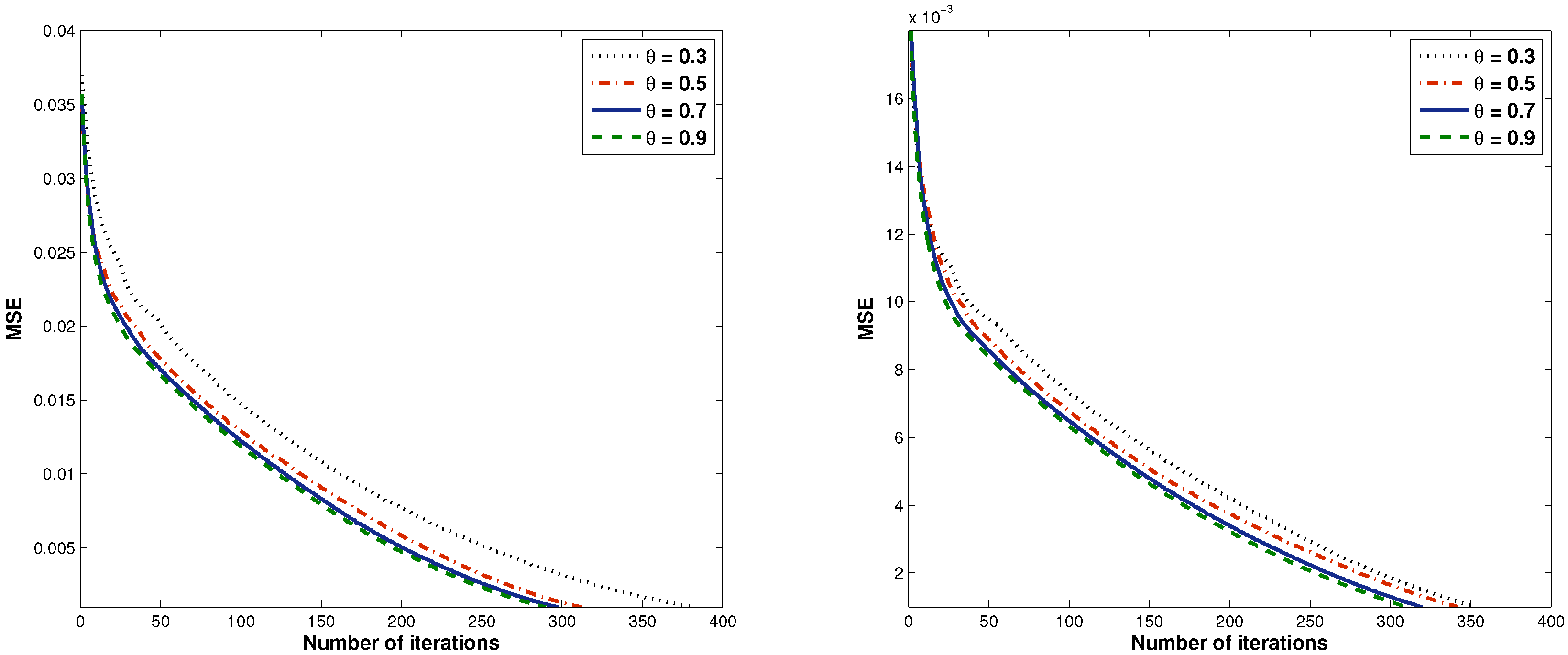
Given: σ = 100, δ = 0.1, γ = 1.9
θN = 512, M = 256
m = 20
N = 1024, M = 512
m = 20
CPUIterCPUIter
0.34.018538213.4732354
0.54.235831222.2328342
0.77.508129827.8198320
0.921.784729085.3605311
Table 4. The convergence of Algorithm 4 with each γ .
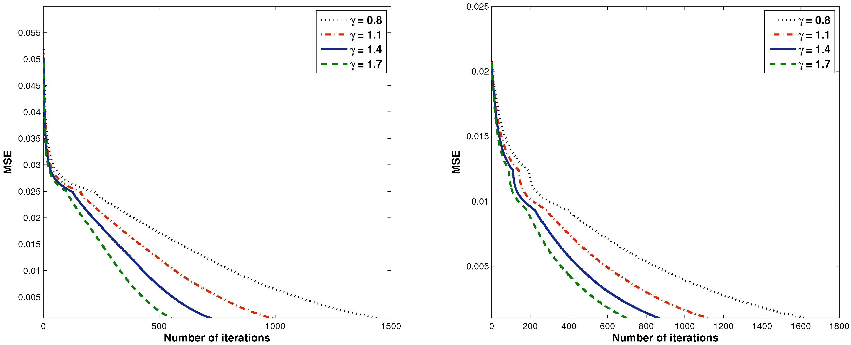
Given: σ = 100, θ = 0.1, δ = 0.1
γN = 512, M = 256
m = 20
N = 1024, M = 512
m = 20
CPUIterCPUIter
0.813.9690145038.27901624
1.17.897898823.34111124
1.45.180472417.6275866
1.73.832355413.6241700
Table 5. The convergence of Algorithm 4 with each σ .
Given: δ = 0.1, θ = 0.1, γ = 1.9
σN = 512, M = 256
m = 20
N = 1024, M = 512
m = 20
CPUIterCPUIter
54.705568011.7794496
306.228084311.3827453
554.427163414.2537532
803.963560616.5507596

