Abstract
In this paper, the effects of strategic consumer behaviors have been investigated and analyzed with regard to online retailers and offline retailers in a dual-channel supply chain. Four channel structures (i.e., no-promotion, a direct online channel, a retail offline channel, and dual channels introduced in the promotion sales period) are considered. At the beginning of the paper, the original demand functions of a dual-channel supply chain incorporating the consumers’ utility has been introduced. The results indicate that despite improved consumer patience, all promotional prices do not fall as expected. When sales channels are provided by online retailers rather than offline retailers during the promotion period, offline retailers can achieve higher profits. We also find that in most cases, a dual-channel model in a single-period is more beneficial to both online and offline retailers than a dual-channel model in two periods, which is, to a certain extent, contrary to the existing literature of single sales channel.
1. Introduction
The Internet has significantly influenced consumers’ purchase patterns. Some consumers may prefer to purchase online, while others may prefer to shop in stores (i.e., offline). Consequently, different consumer purchase patterns have inspired online and offline retail channels (i.e., dual channels). According to eMarketer (2018), e-retail sales accounted for 10.2 percent of all retail sales worldwide in 2017 and expected to reach 17.5 percent in 2021. However, prices for products tend to be marked down after new versions of products are introduced into the market. Notably, about 50% of inventory is sold at discount prices in the clothing industry [1]. Purchasers of automobiles, home appliances, and other durable goods also routinely wait for prices to fall. There are several different kinds of channel structures in current marketing systems to sell overstocked products, such as the traditional offline retail only, the online only, and dual-channel promotion, which is a combination of the first two channels. According to Adobe Analytics Data, Cyber Monday, acting as the most classic online promotional activities in the second sales period, sales topped $7.9 billion in 2018. Black Friday is one of the representative offline promotional activities, and shoppers spent nearly $6.22 billion on the day, 23.6% up from last year. Another example is the Christmas or Chinese New Year, during which both the offline and online retailers intend to offer big discounts. These examples demonstrate the effectiveness of online and offline promotional strategies.
These observations motivated us to explore the impact of channel market structure on how an offline/online retailer makes strategic decisions to clear overstocked products in the second period. In this paper, a two-period model for the online and offline channels that sell the same products has been developed. In the first sales period, regular-priced products are sold in both the offline channel and the online channel at the same time, while in the second sales period, overstocked products are sold at discounted prices through three different channel structures: the direct online channel only (defined as “Model D”), or the retail offline channel only (defined as “Model R”), or both channels (defined as “Model B”). In addition, we also wondered whether the extended sales period is beneficial to the retailers by considering no promotion situation (defined as “Model N”). In each model, we are interested in investigating the effects of strategic consumers’ behaviors on the whole system equilibrium.
We characterize the strategic consumers’ behaviors, including the degree of consumer patience and the acceptance of the direct channel into two-period offline/online channel sales models. Whether consumers purchase during the first or second sales period mainly depends on the degree of consumer patience. Consumers may wait for the lowest possible discounted price before making a purchase [2]. According to the Market Research Society’s survey, more than 50% of consumers tend to wait for the low-price period to buy products. In addition, the acceptance of the direct channel reflecting consumers’ willingness to purchase online is a key factor. When strategic consumers confront dual channels, consumer acceptance of the direct channel may be less than the acceptance of conventional retail stores because delivery time exists in a direct channel.
We construct a Nash game-theoretic model to represent the interaction among the online retailer, the offline retailer, and a population of strategic consumers in the four above-mentioned channel market structures. The contribution of this study is threefold. First, demand functions at each sales period through offline or online channel are firstly introduced by incorporating the consumer’s utility in our paper. Second, optimal quantity strategies for the online and offline retailers in four dual-channel supply chains are established, respectively. Third, the pricing decisions and profits of online and offline retailers among different sales channel structures are compared to judge whether offline or online channel in the second sales period should be offered or which model should be adopted.
We make some interesting observations. First, even though the degree of consumer patience increases, all selling prices in the promotion period set in Model D, Model R, and Model B do not decrease as expected. Meanwhile, the offline retailer’s optimal quantities and prices do not always decrease with the increase in the acceptance of the online channel. In particular, the offline retailer’s results in the promotion period increase with increasing acceptance in Model R. Second, the online retailer’s profit and offline retailer’s profit in Model B are lower than those in Model N, respectively, which is contrary to the results reported in the existing literature. Third, compared with introducing an offline channel in the promotion period by the offline retailer (i.e., Model R), the offline retailer could obtain higher profit when the online retailer sets the online channel in the promotion period (i.e., Model D).
The remainder of this paper is organized as follows. Section 2 reviews the relevant literature. Section 3 introduces the innovative demand functions of the four models described above. Section 4 derives the optimal decisions of online and offline retailers for the different retail structure strategies. Section 5 compares the equilibrium results of the different retail structure strategies by numerical examples. Section 6 concludes the results and outlines limitations. Finally, Appendix A presents the proofs for the Propositions.
2. Literature Review
Our paper focuses on the research of an offline/online dual channels supply chain. The dual-channel supply chain with a single-period model has been given much attention, mainly on channel choice. Arya et al. (2007) showed that the online channel plays an important role in exerting potential competition pressure on the existing retailer by increasing the manufacturer′s negotiation power [3]. Moreover, Chiang et al. (2013) found that the introduction of an online channel always results in a wholesale price reduction, which might benefit both the retailer and the manufacturer [4]. Li et al. (2019) investigated the strategic effect of return policies in a dual-channel supply chain where the manufacturer decides whether to implement a return policy in the online channel, the offline channel, and dual channels [5]. However, only one single sales period is considered in these essays; we concentrate on the channel choice in the promotion sales period, which has seldom been touched. A considerable body of research also concentrates on pricing strategies in the dual-channel supply chain. Hua et al. (2010) examined the optimal decisions of a dual-channel model under the condition of the linear demand function, but they did not take strategic consumers into account [6]. Many other factors, such as delivery lead time [7], product availability for offline channel’s service [8], return policy adoption [5,9], are considered to examine how these factors affect the whole pricing strategy of dual channels.
A significant amount of work has been carried out on the two-period model. De Giovanni and Zaccour (2014) investigated the pricing, collection effort decisions, and members’ profitability to compare several two-period closed-loop supply chain configurations of the collection process [10]. Lin (2016) assumed that the demand function is linear and includes reference price effects, they found the reference price effect could alleviate the double marginalization effect and improve the channel efficiency [11]. In the same demand setting, Maiti and Giri (2017) developed four decision strategies, including the same or different wholesale prices to two selling periods in preannounced or delayed pricing strategies [12]. When the demand at each period is stochastic, Chen and Xiao (2016) investigated the optimal decisions of the players, where stock-out and holding costs are incorporated into the two-period model [13]. However, neither of these studies addressed price-dependent demands by introducing strategic consumers’ behavior, such as consumers’ patience. Papanastasiou and Savva (2017) touched upon the consumer degree of patience in the two-period supply chain [14]. But they ignored the strategic behaviors in the dual channels model.
By combining the dual-channel with a two-period supply chain, we observed studies on the two-period dual-channel supply chain, which are also closely related to this paper. For instance, Lai et al. (2010) investigated the price matching strategy, which eliminates the enthusiasm of consumers to delay buying, thus allowing retailers to increase prices during normal sale periods [15]. Huang et al. (2012) developed a two-period pricing and production decision model in a dual-channel supply chain that experiences demand disruption during the planning horizon. They showed that optimal prices are affected by consumers’ channel preferences and the market scale [16]. Nevertheless, what we obtained reveals that the optimal pricing structure also depends on the degree of consumer patience. Xiong et al. (2012) considered a durable goods market consisting of direct sales by manufacturers through online and offline channels and a mix of selling and leasing by dealers through the offline channel to consumers [17]. In the same setting with [17], Yan et al. (2016) investigated how the addition of the online channel affects the traditional marketing strategies of leasing and selling [18]. The previous literature do not consider strategic consumer behaviors.
There has been a growing interest in studying the impact of strategic consumer behavior on a seller’s pricing decision. Hübner et al. (2013) structured retail demand and supply chain planning questions coherently from the perspective of suppliers and consumers [19]. In Cachon and Swinney (2009), consumers may wait for a clearance sale, the probability of which is low if the seller can better match supply with demand using advance demand information [20]. In our paper, both the acceptance of the online channel and the degree of consumer patience for waiting for the second sales period are discussed in a dual-channel supply chain. Furthermore, strategic consumer behaviors are also discussed in other marketing settings. For example, Giampietri et al. (2018) investigated consumer’s motivations and behaviors in a short food supply chain [21]. Zimon and Domingues (2018) developed guidelines for the concept of sustainable supply chain management in the textile industry [22]. Zhou (2016) focused on the pricing strategy of a dual sales channel where the price in the second period has no effect on the market demand in the first period [23]. By contrast, this effect is elaborated in our model. We also incorporate the effect of several channel structures on profits to provide insights for the choice of sales structure.
To the best of our knowledge, the supply chain with dual-channel, two sales periods, and strategic consumers described in this paper has seldom been studied. For the problem described above, we characterize the degree of consumer patience and the acceptance of the direct channel into a two-period dual-channel sales model. We also present a numerical analysis for choosing the optimal channel structural strategy.
3. Models
In this section, we describe the basic model of consumer choice and the demand functions within different channel structures over two periods in detail.
3.1. Online and Offline Retailers
This paper focuses on four common models, online and offline retailers would have four different quantitative behaviors. The first model is a benchmark model without considering the second promotion period (denoted “Model N”). In the second model (denoted “Model D”), only the online seller provides a price discount in the second period. This setting is motivated by the online promotion on “Cyber Monday” in the United States or “Double Eleven” in China. Inspired by store promotion on “Black Friday”, some offline retailers promote products in the second period (denoted “Model R”). At last, both the retailers adopt promotion strategies in dual channels (denoted “Model B”). Figure 1 presents the sequence of events under the four models.
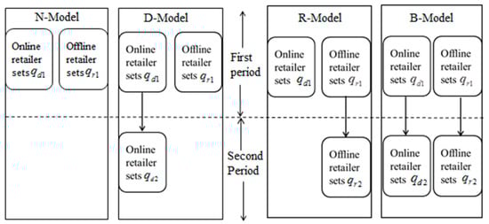
Figure 1.
Graphical representation of decision sequences for four models.
The interactions between the online retailer and offline retailer are modeled by using the Nash game theory. The online and offline retailers announce retail quantities and , respectively, and simultaneously at the beginning of the first sales period, then in the promotion sales period, the online retailer and offline retailer set the retail quantity in Model D, or quantity in Model R, or and in Model B.
Correspondingly, the prices of online and offline retailers in the first sales period are and , respectively, and the discount prices in Period 2 are and . Due to the delivery delay in the online channel, consumers may expect that the price in the online channel is less than that in the offline channel to balance the disadvantage, i.e.,
We refer to the first selling period as the full-price period and the second selling period as the promotion period, that is,
We also consider that in this dual-channel supply chain, firms are risk-neutral, and the information between the two channels is symmetric. Finally, we follow the literature (e.g., [24,25]) to normalize the production and selling costs of the products to zero.
3.2. Strategic Consumers
On the one hand, a product is worth subject to a real inspection while immediate possession has worth when the product is obtained from the direct channel due to the delivery delay in the online channel. Here parameter is called the consumer acceptance of the direct channel. Specifically, when approaches to 1, it indicates that the delivery time is very short, and the consumer tends to fully accept the direct channel, and vice versa. On the other hand, patient consumers may decide to buy products in the second period and wait until the price is low enough. To incorporate this behavior, parameter is used to interpret as a measure of the consumer′s patience. As with [8,26], the parameter could also be explained as product availability in the second period because there exists out of stock in the second period. The structure of the consumer utility function here is the same as in the above-mentioned literatures. Since we focus on strategic consumers’ behaviors in our paper, we define it as the degree of consumer patience. Throughout the analysis, a consumer is “myopic” when and “infinite” when approaches to 1 [14]. The acceptance of online channel arises from the delay due to the delivery time in the online channel. Consumers are willing to wait more time for the second-period promotional activities to get low prices; thus, for the same products, consumers would obtain a smaller discount when buying from the second period in comparison to buying from the online channel, which means as they are both referring to the delay in consumption.
Strategic consumers are homogenous in the valuation of products, the consumption value (alternatively called “willingness to pay”) is assumed following uniformly distributed on [0,1] within the consumer population. Thus, a consumer evaluates four expected utilities of different strategies as follows.
- (1)
- Buy at the beginning of the first selling period (denoted “Period 1”) through the offline retail channel, which yields an expected utility of .
- (2)
- Buy at the beginning of Period 1 through the direct online channel, which yields an expected utility of .
- (3)
- Wait for the second selling period (denoted “Period 2”) through the offline channel, the expected utility is ;
- (4)
- Wait for the second selling period (denoted “Period 2”) through the online channel, the expected utility is .
Where is the price of the channel in Period , where and . Here and denote the direct online channel and offline retail channel, respectively.
3.3. Demand Functions
We need to analyze consumers’ choice when products can be purchased in dual channels in both periods on four common scenarios: Model N, Model D, Model R, and Model B. Figure 2 illustrates the utility functions in the case of these models.
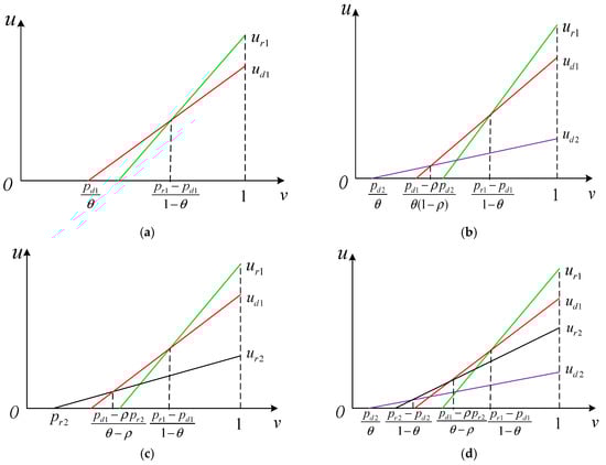
Figure 2.
Consumer utilities. (a) Model N; (b) Model D; (c) Model R; (d) Model B.
Generally speaking, (or ) is a threshold value that consumers have a positive utility buying through an online channel (or an offline channel) in Period 2. The consumer who is indifferent between buying products through an offline channel and an online retail channel in Period 1 is located at , which could be observed intuitively in Figure 2a. Then, for a consumer who prefers the online channel in Period 1 to the online channel in Period 2. The consumer’s valuation should exceed , which is shown in Figure 2b,d. Next, from Figure 2c,d, we can obtain that each consumer whose valuation exceeds would consider buying from the online retailer in Period 1 rather than buying in the offline channel in Period 2.
Thus, with the help of consumer utilities and Figure 2, we obtain the demand functions in each model. In Model N, the demand functions of the online and offline retailers are as follows:
For the situation of Model D, the demand functions are
In the case of Model R, the demand functions are
Lastly, in Model B, the demand functions are
4. Model Analysis
In this section, we model the game and analyze the equilibrium outcomes under the four different scenarios (as described in Section 3.1) when the online and offline retailers conduct the Nash game, where firms choose quantities rather than prices, e.g., [3,17,24,27].
4.1. No Promotion Model (Model N)
Here, we discuss the scenario that the second period is not introduced. This scenario is used as a benchmark model with which to compare the three subsequent models. In Model N, the demand function is shown in Equation (1). Hence, the reverse function is
In this benchmark model, the online and offline retailers decide their retail quantities at the same time. The profit functions of online and offline retailers are as follows:
Therefore, the equilibrium results are obtained as the following proposition.
Proposition 1.
In Model N, the online and offline retailer’s optimal sales quantitiesandare,. Corresponding, the optimal prices are, .
Proof.
For given and , calculate the first derivate of on and , respectively. We have , , therefore, there exists a unique optimal pair , . Substituting and into , , the prices in dual channels are , . □
Arya et al. (2007) studied the same problem as in Model N without considering strategic consumers [3], while in our paper, we examine how acceptance of the online channel affects the whole pricing strategy of dual channels. Proposition 1 elaborates that in Model N, the sale price decided by the online retailer increases with rising acceptance of the online channel. Intuitively, as the competitor of the online retailer, the performance of offline retailer results has declined with the increasing acceptance of the online channel. This observation is partly consistent with the property of the offline retailer in Chiang et al. (2003) [4]. They stated that when acceptance of the online channel is below a cannibalistic threshold, the optimal prices and quantities are not influenced by the acceptance of the online channel. However, we further find that the acceptance of the online channel plays an important role for the online retailer no matter how small of consumer acceptance of the direct channel is.
4.2. Direct Online Channel Introduced in Period 2 (Model D)
This subsection considers Model D, in which the offline retailer does not do any promotions, and their second-period price is the same as the price in Period 1. As a result, their second-period sales volume is zero. In the case of Model D, the online and offline retailers’ demand functions are stated by Equation (2). Hence, the reverse demand functions are
The online retailer and the offline retailer interact as follows: the online retailer determines the optimal sale quantity , and the offline retailer chooses the optimal sale quantity at the same time in Period 1. Then the online retailer decides the sales quantity sold through the direct online channel in Period 2.
We then use backward induction to determine the perfect equilibriums. Proposition 2 shows that there exists a unique Nash equilibrium for this model.
Proposition 2.
There exists a unique Nash equilibrium in the Model D
Further, the corresponding optimal prices in Period 1 and solutions in Period 2 are
Proof.
See Appendix A. □
Zhou (2016) also studied the pricing problem in a dual-channel considering online promotion [19]. They focused on the relationship between selling cost advantages and price strategies chosen by retailers, while we concentrate on the effects of consumers’ strategic behaviors on the optimal quantities and prices of retailers. Following the preceding discussion of the optimal decisions in Model D, the following propositions are provided.
Proposition 3.
In Model D, , , and, , , .
Proof.
See Appendix A. □
Proposition 3 shows that when the acceptance of the online channel is high, or consumers prefer to wait, online retailers strategically raise the price in Period 2 to obtain a high marginal benefit. What is more, as consumers become more patient, the online retailer extends the sales volume in Period 2 and reduces it in Period 1 in response to alleviate the competition pressure with the offline retailer in Period 1. From the offline retailer’s viewpoint, offering an online channel in Period 2 is a serious threat to the offline retailer. To compete against the online channel and protect its market share, the offline retailer has to cut its retail price as the only effective tool. Thus, the offline retailer’s sales volume increases. Finally, as the direct channel becomes more attractive, more consumers would choose to buy from the online channel instead of the offline channel.
4.3. Retail Offline Channel Introduced in Period 2 (Model R)
In Model R, the online and offline retailers’ demand functions are stated by Equations (3). Thus, the reverse functions in Model R are
The behaviors of two retailers in Model R in Period 1 are similar, as in Model D. Proposition 4 shows that there exists a unique Nash equilibrium for Model R.
Proposition 4.
In the Model R, the optimal retail quantities in Period 1 are
Further, the corresponding optimal prices in Period 1 and equilibrium solutions in Period 2 are
Proof.
See Appendix A. □
Following the preceding discussion of the optimal decisions in the Model R, the following propositions are provided.
Proposition 5.
In Model R,, , , , and, , .
Proof.
See Appendix A. □
In the offline channel, more patient consumers in Period 1 would shift to purchase in Period 2. As a result, the sales volume through the offline channel in Period 1 decreases with the degree of patience, while the sales volume in Period 2 increases. But it seems counter-intuitive that more patient consumers will not wait for lower prices in Period 2. Confronted with patient consumers, offline retailers’ marketing strategy of setting a high price in Period 2 aimed at attracting consumers to purchase in Period 1 since they could obtain a high marginal profit in Period 1 since .
Propositions 5 also shows that when the offline retailer extends the selling period, confronted with more patient consumers, the offline retailer sets a lower selling price to avoid reducing fierce competition in Period 1. Then the online retailer has to cut its selling price to protect its market share. Accordingly, the online retailer’s sales volume in Period 1 increases with respect to the degree of patience, which is symmetric with properties of offline retailer’s sales volume in Model D, as shown in Proposition 3.
Contrary to the existing literature of single sales period, Chiang et al. [4] and Xu et al. [7] verified that offline retailers’ price is negatively correlated with the acceptance of online channels. Propositions 5 shows that in Period 2, the offline retailer aggressively increases prices to make the competition more intense with the rising acceptance of the online channel, the main reason is that the offline retailer occupies the entire second-period market in Model R.
4.4. Both Channels Introduced in Period 2 (Model B)
In Model B, the online and offline retailers’ demand functions are stated by Equation (4), it follows that the reverse demand functions are
We discuss the optimal quantity decision in Model B, which means that the first-period and second-period sales quantities will be announced at the beginning of the corresponding selling period. Using backward induction, Proposition 6 shows that a unique Nash equilibrium exists for Model B.
Proposition 6.
In Model B, the optimal retail quantities in Period 1 are
Further, equilibrium solutions in Period 2 are
The corresponding optimal prices in Period 1 and Period 2 could be obtained by Equations (7).
Proof.
See Appendix A. □
5. Discussion and Comparison
In this section, the effect of strategic consumer behaviors on optimal results in Model B is discussed, and the optimal results obtained under four different decision strategies are compared.
5.1. Sensitivity Discussion
First, take a closer look at the implications of consumer patience for two parties’ outcomes in Model B. When the acceptance of the direct channel is given, taking , the properties of sales volumes and prices about , will be represented in Figure 3 and Figure 4. Taking , we obtain the properties of sales volumes and prices about , , which are shown in Figure 5 and Figure 6, respectively.
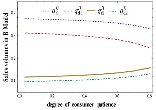
Figure 3.
Impact of on sales volumes in dual channels Model B.
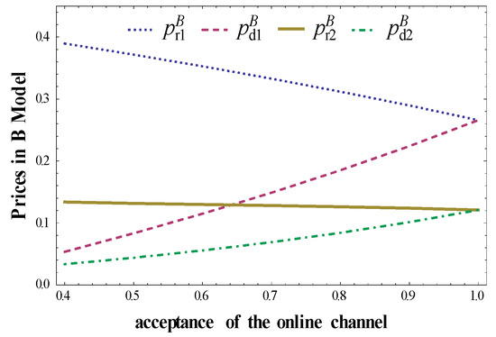
Figure 4.
Impact of on prices in Model B.
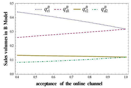
Figure 5.
Impact of on sales volumes in Model B.
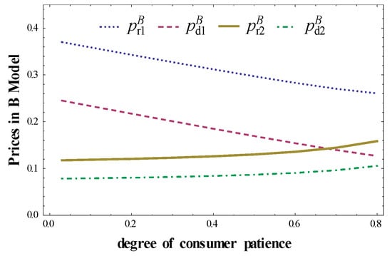
Figure 6.
Impact of on prices in Model B.
Some discussions about these figures are given in the following:
In Model B, Figure 3 and Figure 4 reveal that sales volumes and prices in Period 1 decrease with the rising degree of patience either from the online or offline retailer. While in Period 2, sales volumes and prices have opposite characters, that is, ,, ,, . The reason for this is that retailers aim at attracting consumers to purchase in Period 1 since they have a high margin in Period 1. This relationship seems to contradict to the expected results from consumers, which suggests that more patient consumers could wait for the lower price. In fact, this interesting phenomenon, that second-period prices decrease as consumer’s patience increases, is also investigated by Papanastasiou and Savva (2016), where they only considered one retail channel in the two-period model [14].
In addition, the price and sales volumes set by the online retailer increase as the acceptance of the online channel increases in both Period 1 and Period 2. While it is the opposite for all the results of the offline retailer, i.e.,, , , , , which is illustrated in Figure 5 and Figure 6. Obviously, this efficient online channel helps increase online prices and forces the offline retailer to markdown retail prices in both selling periods, which is different from the results in Model R. Proposition 5 stated that the offline retailer aggressively increases the offline second-period price as online channels gain acceptance because the offline retailer occupies the entire market.
5.2. Comparison of Dominating Areas
In this section, we graphically show some regions with the pair of parameters where we compare selling quantity sequences in Period 1, the online retailer’s profit sequences, and offline retailer’s profit sequences under four different models. Some discussions about these figures are given in the following.
First, the relationship of offline quantities and online prices with respect to the acceptance of the direct channel will be examined by numerical experiments by taking in the left-hand of Figure 7, Figure 8, Figure 9 and Figure 10. Similarly, we set in the right-hand of Figure 7, Figure 8, Figure 9 and Figure 10 to investigate the offline quantities and online prices regarding the degree of consumer patience. The conclusion could be graphically obtained without any assumption in region , but it is not clear in 3-Dimension situation. Thus, we assume or , respectively, to investigate the properties in 2-Dimensional figures. From Figure 7, Figure 8, Figure 9 and Figure 10, in the region , the quantity and price sequences in Period 1 under four models are stated in the following proposition.
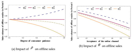
Figure 7.
Offline quantities sequences in four sales strategies.
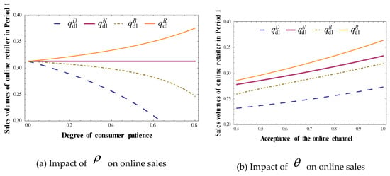
Figure 8.
Online quantities sequences in four sales strategies.
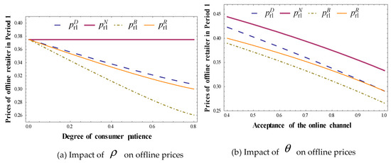
Figure 9.
Offline prices sequences in four sales strategies.
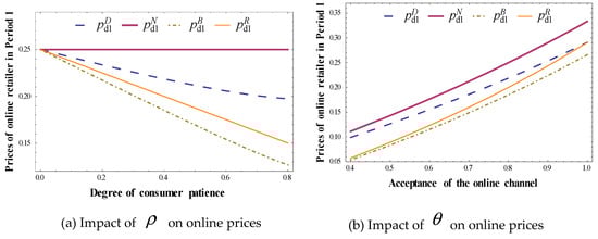
Figure 10.
Online prices sequences in four sales strategies.
Figure 7, Figure 8, Figure 9 and Figure 10 verify the monotonic properties of quantities and prices with respect to parameters, as stated in Propositions 3, 5 and 7. The acceptance of the online channel has a positive impact on online retailer’s prices and quantities, while it has a negative impact on the offline retailer’s prices and quantities. All quantities in Period 1 except for offline retailer’s quantity are decreasing with the increase in the degree of consumer patience because of inter-periodic competition. However, counter-intuitively, as shown in the left-hand of Figure 7, the sales volume of the offline retailer increases with the increase in the degree of consumer patience in Model D. In Model D, offering the online channel in Period 2 is a serious threat to the offline retailer. To compete against the online channel and protect its market share in Period 1, the offline retailer has to cut its retail price as the only effective tool even confronted with patient consumers. Thus, the offline retailer’s sales volume increases. As displayed in the left-hand of Figure 8, the sales volume of the online retailer also increases with increasing degree of consumer patience in Model R for a similar reason.
Some discussions about quantities or prices sequences in these figures are given in the following:
- , . Specifically, the online or offline retailer would achieve higher sales quantities when the second-period promotion sales are provided by its competitor rather than itself.
- , . That is, offline and online retailers have the same price sequence. Further, the retail price without promotion strategy is the highest.
It reveals that the first-period quantity of the online retailer is highest when sales promotion is provided by the offline retailer; the offline retailer also has a symmetrical property. This is partly because there is no chance for consumers to purchase through the online channel in Period 2 in Model R. Moreover, sales quantities of both the online retailer and the offline retailer reach their second-highest in Model N and third-highest in Model B. On the other hand, their second-highest prices are obtained in Model D. Channel competition only exists in Model N, the online and offline retailers set the highest prices in Period 1 in Model N, while channel competition and periodic competition both exist in Model B, retailers set the lowest prices in Model B. We can thus conclude that Model N or Model D will be preferable for online and offline retailers as they set high volumes and prices for the first period, which will be verified below.
Similar to Arya et al. [3] and Xiong et al. [17], compared with only the offline channel setting, the manufacturer, also acting as an online retailer, may offer a lower wholesale price to the downstream retailer in the dual-channel setting. Our results also show that, compared with promotion only through the offline channel (i.e., Model R), the online retailer would set a lower first-period price when promoting sales through dual channels (i.e., Model B) to offset the advantage of online retailer’s competitive position in the retail market. Among other results, we found that the first-period price was always higher in Model D than that in Model R. Moreover, Erhun et al. [28] stated that the first-period price increases as the number of selling period increases. However, we show that the first-period price in the single-period setting (i.e., Model N) is the highest.
Without any assumptions, we can graphically summarize the detailed profit sequences of the online and offline retailers under four different strategies in the following figures.
From the region shown in Figure 11, the online retailer in Model N dominates in terms of profit. is the secondary dominator when and take higher values, or is the secondary dominator when and take lower values. Surprisingly, is always the lowest in all regions except for the higher values for and , where is the minimum. For the offline retailer, dominates when and is higher, but when takes lower values irrespective of the value, dominates others. In the region that Model D dominates, is the secondary dominator and is the minimum. While in the region that Model N dominates, is the secondary dominator and is the minimum (see Figure 12).
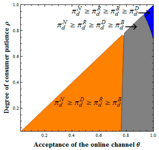
Figure 11.
Online retailer’s profit sequences under four sales strategies.
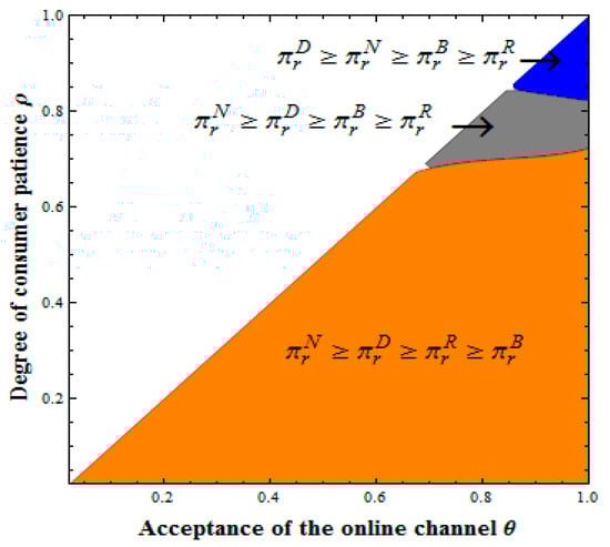
Figure 12.
Offline retailer’s profit sequences under four sales strategies.
The optimal channel structure strategy depends on the players confronting which types of consumers. In summary, the best choice for the online retailer is Model N, while it is better to choose Model N or Model D than Model R or Model B for the offline retailer. In particular, compared with providing an offline channel in Period 2 by themselves, the offline retailer could get higher profits when the online retailer introduces the online channel in Period 2. The main reason is that the offline retailer’s selling quantity and price in Period 1 in Model D are initially higher than those in the Model R. Practically speaking, offline retailers would be more enthusiastic on Cyber Monday and Double Eleven than even Black Friday.
Contrary to the conventional wisdom, Erhun et al. (2008) stated that all members within the supply chain benefit from multi-period trading [28]. Figure 11 and Figure 12 imply that bearing the brunt of the online channel, single-period selling dominates two-period selling in the dual-channel supply chain. In other words, the profits of online and offline retailers in the single-period dual-channel model (i.e., N Model) is always higher than those in the two-period dual-channel model (i.e., B Model). Thus, offering dual channels in the promotion period will not make the best strategy. We believe this difference stems from the competition between online and offline retailers rather than the competition between the upstream manufacturer and the downstream retailer.
On the other hand, Figure 11 shows that, from the online retailer viewpoint, compared with only the offline channel existing in the second period (i.e., Model R), the introduction of the online channel in the second sales period (i.e., Model B) cannot create a higher profit. Figure 12 also shows that the offline channel achieves a higher profit in Model D rather than in Model B. Our observation differs from the observation of Chiang et al. [4] and Chen [29] who argued that “introducing the online channel model provides the online retailer’s profit improvement”. They focus on determining the optimal selling price in a single-period supply chain while we consider the pricing policy in a two-period supply chain.
6. Discussion and Comparison
Dual-channel distribution systems, including an online channel and an offline channel, have been adopted by many retailers (defined as “Model N”). Retailers consider setting the promotion period to sell products through only the online channel, or only the offline channel, or dual channels at the same time (defined as “Model D”, “Model R”, and “Model B”, respectively). Although the marketing issues associated with two selling periods have been well studied, limited results are known about how these marketing strategies are influenced by the retailers’ adoption of different channel structures and the penetration of strategic consumers. To fill in this gap, this paper attempts to investigate how strategic consumers’ behaviors impact the optimal quantities and how the retailers’ selling strategies affect their profits.
We first introduced four original demand functions of the dual-channel supply chain by incorporating the consumers’ utility in our paper. Based on it, we establish optimal quantity and price strategies for online/offline retailers. Our results indicate that, in most cases, all online retailer’s optimal sales volumes and prices increase as the acceptance of the online channel increases, while it is opposite for the offline retailer. But in Model R, the offline retailer’s optimal decisions in the second period increase with the increase in the acceptance of the online channel. In addition, opposite to all results in Period 1, all volumes and prices obtained in Period 2 increase with the degree of patience increasing. It seems counter-intuitive that a more patient consumer would not wait for a lower price in Period 2.
At last, the equilibrium outcomes of both parties are analyzed among four different channel structure strategies by graphical analysis. We found that strategic consumers’ behaviors (i.e., the acceptance of the online channel and the degree of patience) could strongly influence the choice of channel structures for online and offline retailers. It reveals that online and offline retailers earn the highest profit in the single-period model except when consumers have a high degree of patience and a high acceptance of the online channel. Finally, the offline retailer could obtain higher profits when the online retailer introduces an online channel in the promotion period instead of providing an offline channel in the promotion period.
In this paper, only the retailers and consumers are considered, while future studies could be extended to consider a manufacturer or supplier to analyze the wholesale price. In addition, consumers are homogenous in this paper. Studies next will consider different types of consumers, for example, experienced and inexperienced consumers, which is closer to real life. Moreover, dynamic modeling would seem to be more appropriate in two-period framework research, so dynamic investigation would be our subsequent research topic.
Author Contributions
Conceptualization, Q.L. and J.H.; writing—original draft preparation, Q.L.; writing—review and editing, Q.L. and F.H.; project administration, J.H. All authors have read and agreed to the published version of the manuscript.
Funding
Natural Science Foundation of China through Grant Number 71873111, 71802100, 71273214 and Humanities and Social Science Project of Education Committee through Grant Number 18YJAZH024.
Conflicts of Interest
The authors declare no conflict of interest.
Appendix A
Proof of Proposition 2.
In Period 2, the online retailer’s problem is to choose the optimal quantity to maximize profit
with and given. Thereafter, the online retailer’s optimal retail quantity
By substituting Equation (A1) into Equation (5), based on it, the profit functions of the online retailer and offline retailer could be expressed as
From the online retailer’s profit, the first term is the revenue from selling in Period 1, and the second term is revenue from Period 2. The profit in Period 2 is multiplied by the degree of patience, which is mainly due to the patience of the consumer working as a discount factor, i.e., the online retailer discounts the profits in Period 2 to get the profit value at the same time point as the value in the Period 1. The first-order optimality conditions are
Solving the above equations, we get
Substituting in Equations (A1) and (5), we obtain , , , as stated in Proposition 3. □
Proof of Proposition 3.
In Model D, for convenience, we define , . Taking the derivative of with respect to , we have
Combined with we can derive Then, taking the derivative of and with respect to ,
we find At last, we consider the properties of sales quantities regarding . By first partial derivatives, we obtain
□
Proof of Proposition 4.
In Period 2, the offline retailer decides the sale quantity sold through the offline channel in Period 2. Using backward induction, the offline retailer’s profit in Period 2 is
Thus, the optimal retail quantity is
Combining (A2) with Equations (6), we could obtain the optimal prices and in Period 1. Therefore, the profits of online and offline retailers are
The first-order optimality condition is
which leads to , . Substituting in Equations (A2) and (6), we obtain , , , as stated in Proposition 4. □
Proof of Proposition 5.
In Model R, define , taking the derivative of all results obtained in proposition 4 with respect to , we learn
Combined with , could be obtained. The other conclusions can be derived by first-order partial derivative easily, so we omit them here. □
Proof of Proposition 6.
Using backward induction, the profits of online and offline retailers can be expressed as
It follows that the optimal solutions can be described as follows
We rewrite the profits of two retailers for and as follows
The derivative of the profit function with respect to the selling quantity is
where , and consequently, we get and as expressed in Proposition 6. Substituting and in (A3) and (7), yields the other optimal results. □
References
- Hardman, D.; Simon, H.; Ashok, N. Keeping Inventory-And Profits-Off the Discount Rack; White Paper Booz Allen Hamilton Inc.: McLean, VA, USA, 2007. [Google Scholar]
- Ji, G.J.; Zhao, Y. Strategic consumer behavior analysis based on dual channels and sale periods. Int. J. u-e-Serv. Sci. Technol. 2015, 8, 135–152. [Google Scholar] [CrossRef]
- Arya, A.; Mittendorf, B.; Sappington, D.E. The bright side of supplier encroachment. Mark. Sci. 2007, 26, 651–659. [Google Scholar] [CrossRef]
- Chiang, W.Y.K.; Chhajed, D.; Hess, J.D. Direct marketing, indirect profits: A strategic analysis of dual-channel supply-chain design. Manag. Sci. 2003, 49, 1–20. [Google Scholar] [CrossRef]
- Li, G.; Li, L.; Sethi, S.P.; Guan, X. Return strategy and pricing in a dual-channel supply chain. Int. J. Prod. Econ. 2019, 215, 153–164. [Google Scholar] [CrossRef]
- Hua, G.; Wang, S.; Cheng, T.E. Price and lead time decisions in dual-channel supply chains. Eur. J. Oper. Res. 2010, 205, 113–126. [Google Scholar] [CrossRef]
- Xu, H.; Liu, Z.Z.; Zhang, S.H. A strategic analysis of dual-channel supply chain design with price and delivery lead time considerations. Int. J. Prod. Econ. 2012, 139, 654–663. [Google Scholar] [CrossRef]
- Chen, K.Y.; Kaya, M.; Özer, Ö. Dual sales channel management with service competition. Manuf. Serv. Oper. Manag. 2008, 10, 654–675. [Google Scholar] [CrossRef]
- Zhang, R.; Li, J.; Huang, Z.S.; Liu, B. Return strategies and online product customization in a dual-channel supply chain. Sustainability 2019, 11, 3482. [Google Scholar] [CrossRef]
- De Giovanni, P.; Zaccour, G. A two-period game of a closed-loop supply chain. Eur. J. Oper. Res. 2014, 232, 22–40. [Google Scholar] [CrossRef]
- Lin, Z. Price promotion with reference price effects in supply chain. Transp. Res. Part E-Logist. Transp. Rev. 2016, 85, 52–68. [Google Scholar] [CrossRef]
- Maiti, T.; Giri, B.C. Two-period pricing and decision strategies in a two-echelon supply chain under price-dependent demand. Appl. Math. Model. 2017, 42, 655–674. [Google Scholar] [CrossRef]
- Chen, K.; Xiao, T. Ordering policy and coordination of a supply chain with two-period demand uncertainty. Eur. J. Oper. Res. 2011, 215, 347–357. [Google Scholar] [CrossRef]
- Papanastasiou, Y.; Savva, N. Dynamic pricing in the presence of social learning and strategic consumers. Manag. Sci. 2016, 63, 919–939. [Google Scholar] [CrossRef]
- Lai, G.; Debo, L.G.; Sycara, K. Buy now and match later: Impact of posterior price matching on profit with strategic consumers. Manuf. Serv. Oper. Manag. 2010, 12, 33–55. [Google Scholar] [CrossRef]
- Huang, S.; Yang, C.; Zhang, X. Pricing and production decisions in dual-channel supply chains with demand disruptions. Comput. Ind. Eng. 2012, 62, 70–83. [Google Scholar] [CrossRef]
- Xiong, Y.; Yan, W.; Fernandes, K.; Xiong, Z.K.; Guo, N. “Bricks vs. Clicks”: The impact of manufacturer encroachment with a dealer leasing and selling of durable goods. Eur. J. Oper. Res. 2012, 217, 75–83. [Google Scholar] [CrossRef]
- Yan, W.; Li, Y.; Wu, Y.; Palmer, M. A rising e-channel tide lifts all boats? The impact of manufacturer multichannel encroachment on traditional selling and leasing. Discret. Dyn. Nat. Soc. 2016, 2016, 2898021. [Google Scholar] [CrossRef]
- Hübner, A.H.; Kuhn, H.; Sternbeck, M.G. Demand and supply chain planning in grocery retail: An operations planning framework. Int. J. Retail Distrib. Manag. 2013, 41, 512–530. [Google Scholar] [CrossRef]
- Cachon, G.P.; Swinney, R. Purchasing, pricing, and quick response in the presence of strategic consumers. Manag. Sci. 2009, 55, 497–511. [Google Scholar] [CrossRef]
- Giampietri, E.; Verneau, F.; Del Giudice, T.; Carfora, V.; Finco, A. A Theory of Planned behaviour perspective for investigating the role of trust in consumer purchasing decision related to short food supply chains. Food. Qual. Prefer. 2018, 64, 160–166. [Google Scholar] [CrossRef]
- Zimon, D.; Pedro, D. Proposal of a concept for improving the sustainable management of supply chains in the textile industry. Fibers Text. East. Eur. 2018, 26, 8–12. [Google Scholar] [CrossRef]
- Zhou, C. Pricing model for dual sales channel with promotion effect consideration. Math. Probl. Eng. 2016, 2016, 1804031. [Google Scholar] [CrossRef][Green Version]
- Li, H.; Leng, K.; Qing, Q.; Zhu, S.X. Strategic interplay between store brand introduction and online direct channel introduction. Transp. Res. Part E-Logist. Transp. Rev. 2018, 118, 272–290. [Google Scholar] [CrossRef]
- Li, G.; Li, L.; Sun, J. Pricing and service effort strategy in a dual-channel supply chain with showrooming effect. Transp. Res. Part E-Logist. Transp. Rev. 2019, 126, 32–48. [Google Scholar] [CrossRef]
- Liu, Q.; Van Ryzin, G.J. Strategic capacity rationing to induce early purchases. Manag. Sci. 2008, 54, 1115–1131. [Google Scholar] [CrossRef]
- Li, H.; Shao, J.; Zhu, S.X. Parallel importation in a supply Chain: The impact of gray market structure. Transp. Res. Part E-Logist. Transp. Rev. 2018, 114, 220–241. [Google Scholar] [CrossRef]
- Erhun, F.; Keskinocak, P.; Tayur, S. Dynamic procurement, quantity discounts, and supply chain efficiency. Prod. Oper. Manag. 2008, 17, 543–550. [Google Scholar] [CrossRef]
- Chen, T. Effects of the pricing and cooperative advertising policies in a two-echelon dual-channel supply chain. Comput. Ind. Eng. 2015, 87, 250–259. [Google Scholar] [CrossRef]


© 2019 by the authors. Licensee MDPI, Basel, Switzerland. This article is an open access article distributed under the terms and conditions of the Creative Commons Attribution (CC BY) license (http://creativecommons.org/licenses/by/4.0/).