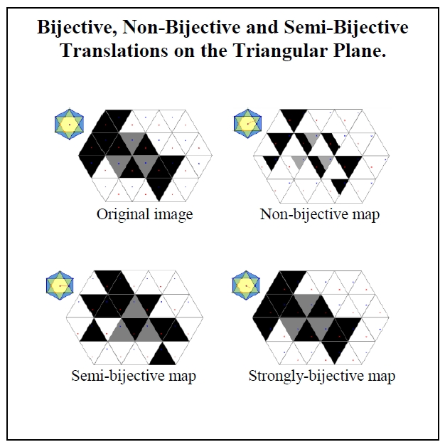
Bijective, Non-Bijective and Semi-Bijective Translations on the Triangular Plane ^†

Abstract

The triangular plane is the plane which is tiled by the regular triangular tessellation. The underlying discrete structure, the triangular grid, is not a point lattice. There are two types of triangle pixels. Their midpoints are assigned to them. By having a real-valued translation of the plane, the midpoints of the triangles may not be mapped to midpoints. This is the same also on the traditional square grid. However, the redigitized result on the square grid always gives a bijection (gridpoints of the square grid are mapped to gridpoints in a bijective way). This property does not necessarily hold on to the triangular plane, i.e., the redigitized translated points may not be mapped to the original points by a bijection. In this paper, we characterize the translation vectors that cause non bijective translations. Moreover, even if a translation by a vector results in a bijection after redigitization, the neighbor pixels of the original pixels may not be mapped to the neighbors of the resulting pixel, i.e., a bijective translation may not be digitally ‘continuous’. We call that type of translation semi-bijective. They are actually bijective but do not keep the neighborhood structure, and therefore, they seemingly destroy the original shape. We call translations strongly bijective if they are bijective and also the neighborhood structure is kept. Characterizations of semi- and strongly bijective translations are also given.

1. Introduction

Digital images consist of a (finite) set of pixels. Thus, both the (re)presentations of the images and the possible operations on them are strictly connected to the underlying grid. Traditionally, the square grid is the most usual one; this is the most known and the most common, partly due to the fact that the Cartesian coordinate frame fits it and fits also its dual grid. However, there are other regular tessellations of the plane, namely the hexagonal and the triangular grids. They are duals of each other (i.e., considering the midpoints of the pixels of one of these grids and connecting the closest neighbor ones, one gets the other grid). They also share several properties, e.g., symmetries. The square grid, even though, traditionally, it is the most used, has some unpleasant properties, e.g., it has a topological (connectivity) paradox, i.e., the two diagonals of the chessboard cross each other without a shared pixel (without a common gridpoint). In the hexagonal grid, there is only one usual neighborhood, and there is no connectivity paradox, thus it gives a nice and simple option in various applications. However, the resolution pyramid does not work well: A hexagonal pixel cannot be cut to smaller hexagonal pixels. A resolution pyramid can be obtained, e.g., by cutting a square or a triangle to four smaller identical ones, using parallel lines to the edges connecting the center points of the edges. We can say that the hexagonal and triangular grids are valid alternatives of the traditional grid both in computer graphics and in digital image processing [1], moreover, in some cases, they could lead to better results than the square grid.

Various transformations including the isometric ones are known from geometry. They are also widely used in computers. However, in the discrete (or digital) world, most of these transformations are not trivial. For instance, Kaufman in a lecture at SigGraph’99 [2] claimed that “Manipulation and transformation of the discrete volume are difficult to achieve without degrading the image quality or losing some information.” By their different properties, discrete and continuous transformations yield two very different theories. The simplest operations on digital images are the (digital or discretized versions of) isomorphic operations, and maybe the most elementary is the translation. Compositions of translations and rotations, on the square and hexagonal grids, have been considered and analyzed, e.g., in [3]. The isomorphic transformations mapping the grid into itself are described on the triangular grid in [4], but transformations that could map some gridpoints out of the grid were not considered. Translations of images are such basic and frequently used operations and usually do not garner any attention alone. One can simply move her or his finger on the screen of her or his mobile/tablet/laptop and various images (icons, signs, or even the whole screen) are translated. Since the square and hexagonal grids are point lattices, any translation by a grid vector is always a bijection from the grid into itself. Also, translations by real vectors can be “rounded” easily to grid translations. In fact, we call this process redigitization, when the corresponding pixels are computed after a translation (or other operation) which may result in some points (of the plane) that are not gridpoints. These types of redigitization play important roles also on the traditional grid when another operation, e.g., discrete rotation is considered, which may not be bijective [3,5]. The triangular grid is not a point lattice (there are grid vectors such that they do not translate the grid into itself, as it is shown in Figure 1), and therefore, as we show here, it is interesting to consider translations and analyze how the resulting image may change. In a nutshell, having translations with various vectors, it may happen that the translation is not bijective, i.e., points with no preimage and points with two preimages appear. In other cases, even the translation is bijective, the translated pictures are displayed in a wrong way due to the fact that neighbor pixels are not mapped to neighbor pixels (we call this case semi-bijective; in terms of digital continuity by [6], even if these translations are bijections, they are not continuous digitally). Finally, there are bijective translations which also keep the figure; in fact, really, they ‘just’ translate it. We call the transformations of this latter case strongly bijective translations.

The digital geometry of the triangular grid is based on various digital distance functions, e.g., neighborhood sequences [7]. The triangular grid was recently applied in various image processing algorithms, e.g., discrete tomography [8] and thinning [9,10]. Thus, thanks to the increasing attention, we feel that it is time also to describe discrete translations on this grid. We believe that our results can be applied in various places from applied mathematics to computer engineering, including, e.g., digital signal processing for computer vision applications.

The structure of the paper is as follows. In the next section, we recall some basic facts about discrete translations on the square grid and define discrete translations on the triangular grid; we also fix our notations. In Section 3, we give technical details for the description of translations on the triangular grid, and in Section 4 we characterize the translation vectors by necessary and sufficient conditions for strongly bijective, semi-bijective and non-bijective translations. Concluding remarks close the paper. This paper is a continuation and extension of our earlier conference paper [11] where non-bijective and bijective translations were presented. Here we also separate two cases of the bijective ones.

2. Preliminaries

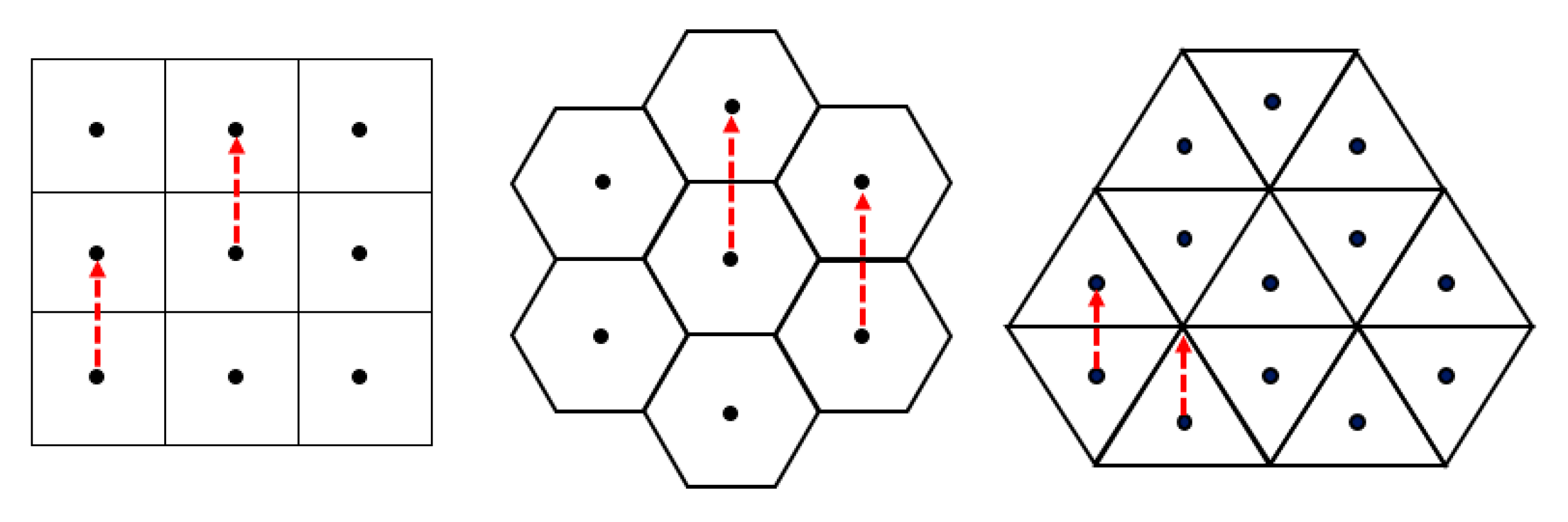
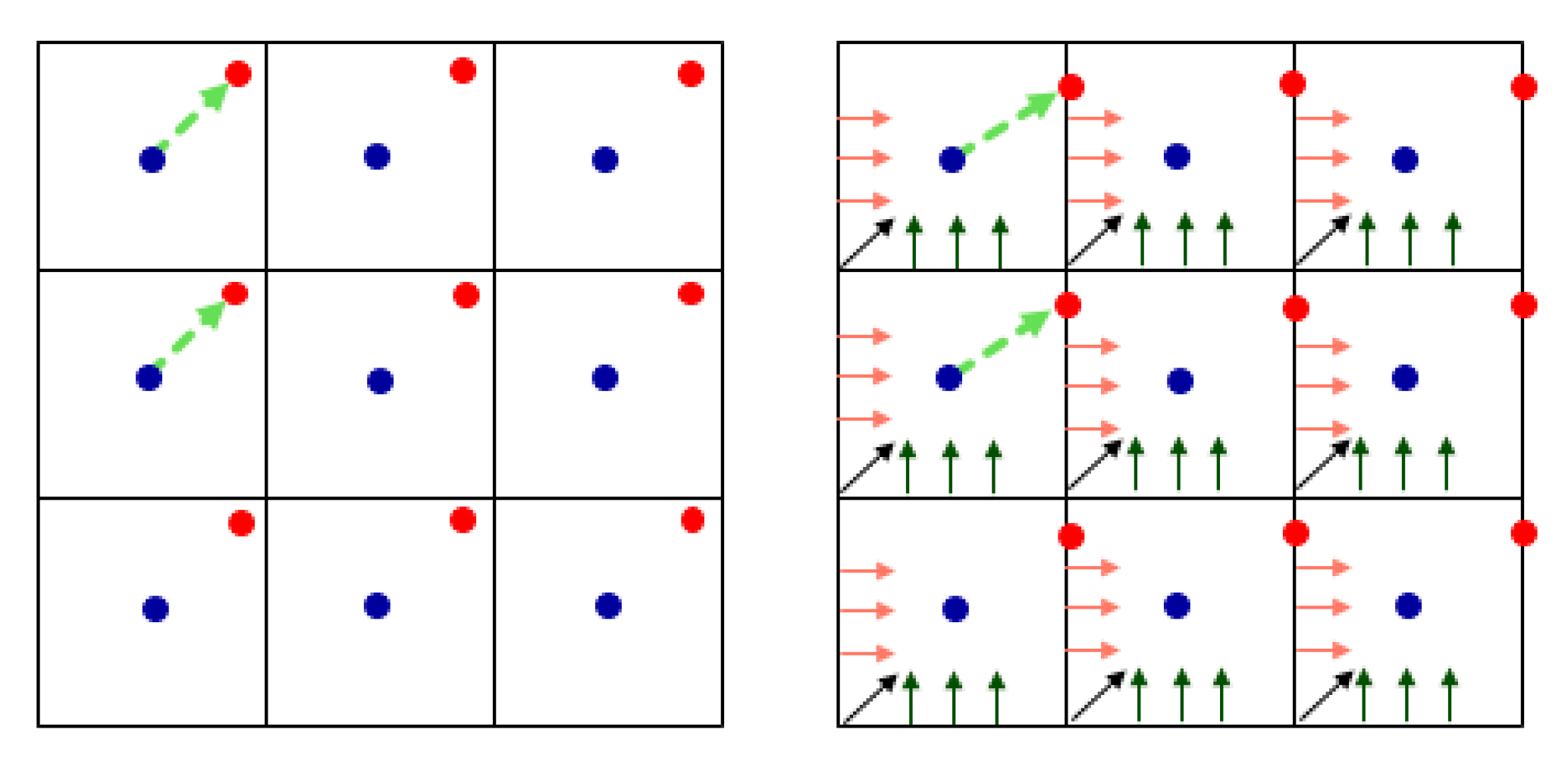
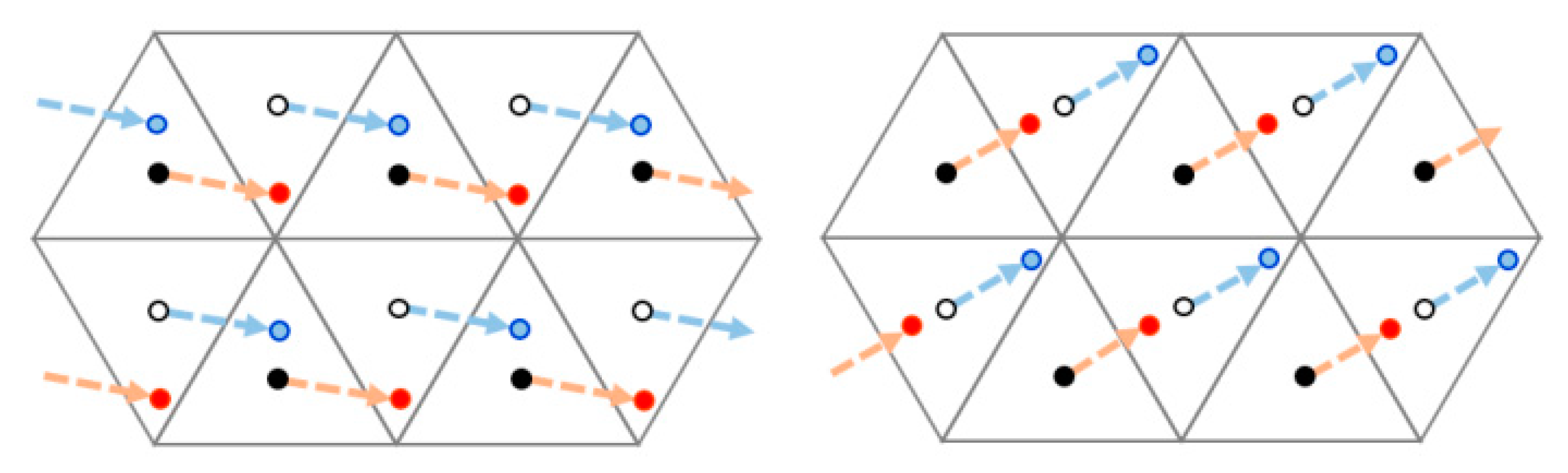
2.1. Discrete Translations

Discrete translations are the discretized forms of the Euclidean translations. They are usually defined as a composition of the Euclidean translation $\tau$ by a given vector, applied on the points of the discrete grid G, and a rounding operator to make sure that the result/the image of the discrete translation belongs to the grid. Digitized translations are, then, formally, usually defined as functions $D_{\tau }=D\circ \tau \left(G\right)$ where both the domain and the target are the given (digital or discrete) grid G.

The discretized translations in the square and the hexagonal grids are always bijective, but they are not always bijective in the triangular grid. This is because when a grid-vector is taken from any gridpoint (of the square or the hexagonal grids), it will always end up at a certain gridpoint, i.e., these two grids are point lattices. Opposite to this, it is not the case when the triangular grid is considered, as an example is shown in Figure 1 (right).

Although the discretized translation in the triangular grid is an extension of the classical Euclidean translation with a rounding operation to the nearest grid midpoint, similar to the cases of the square and hexagonal grids, the translation on the triangular grid has never been discussed or characterized in detail. Only specific translations have been introduced, as somewhat integer translations, with the property that the gridpoints are mapped to gridpoints [4].

In order to analyze discretized translations, two basic concepts must be defined/recalled first, the surjective and injective translations. We generally use the set E which could be the Euclidean plane/space or a discrete space (e.g., the square grid). We remind the reader that the translation as a function may have the following properties:

A translation $f:E\to E$ is

• surjective if $\forall i\in E$ in the target, there is at least one element $i^{\prime }\in E$ in the domain, such that $f\left(i^{\prime }\right)=i$.
• injective if $\forall a,b\in E$ in the domain, whenever $f\left(a\right)=f\left(b\right)$ then a = b. Formally:

  $$\forall a,b\in E, f\left(a\right)=f\left(b\right)⟹a=b.$$
• bijective if it is both injective and surjective.

It is well known and one can easily check that every translation is bijective on the square grid (see Figure 2, for examples). In the next subsection, we give some formal details.

Translations on the Traditional Grid

The translation by a vector t(t_x, t_y) $\in$ ${ℝ}^2$ in the two-dimensional Euclidean space, i.e., in the plane is the function f ${ℝ}^2$ → ${ℝ}^2$ such that f(x, y) = (x + t_x, y + t_y). On the square grid, discrete translations are defined analogously, but changing the domain and the target of the function f to ${\mathbb{Z}}^2$. Moreover, usually not only integer translation vectors are allowed, but any vector t(t_x, t_y) $\in$ ${ℝ}^2$ and, then a rounding operator is used for both coordinates to assign the closest gridpoint to the resulting point. Analogously, (t_x, t_y) = (x₀, y₀) + (x₁, y₁), where (x₀, y₀) is the integer vector to the closest gridpoint to t, and (x₁, y₁) is the fractional vector within the grid-square where $-0.5 \le x_1,y_1<0.5$. Then the rounding operator will be defined by the help of the floor function:

$$\left(⎣x_1+\frac{1}{2}⎦,⎣y_1+\frac{1}{2}⎦\right).$$

This can also be seen as, based on the square tessellation of the grid, to assign the midpoint of that pixel to the translated point for the pixel to which the point belongs. For those translated points that are on the borders of a square tile in the grid, the rounding operation is systematic and obvious (see Figure 2 right).

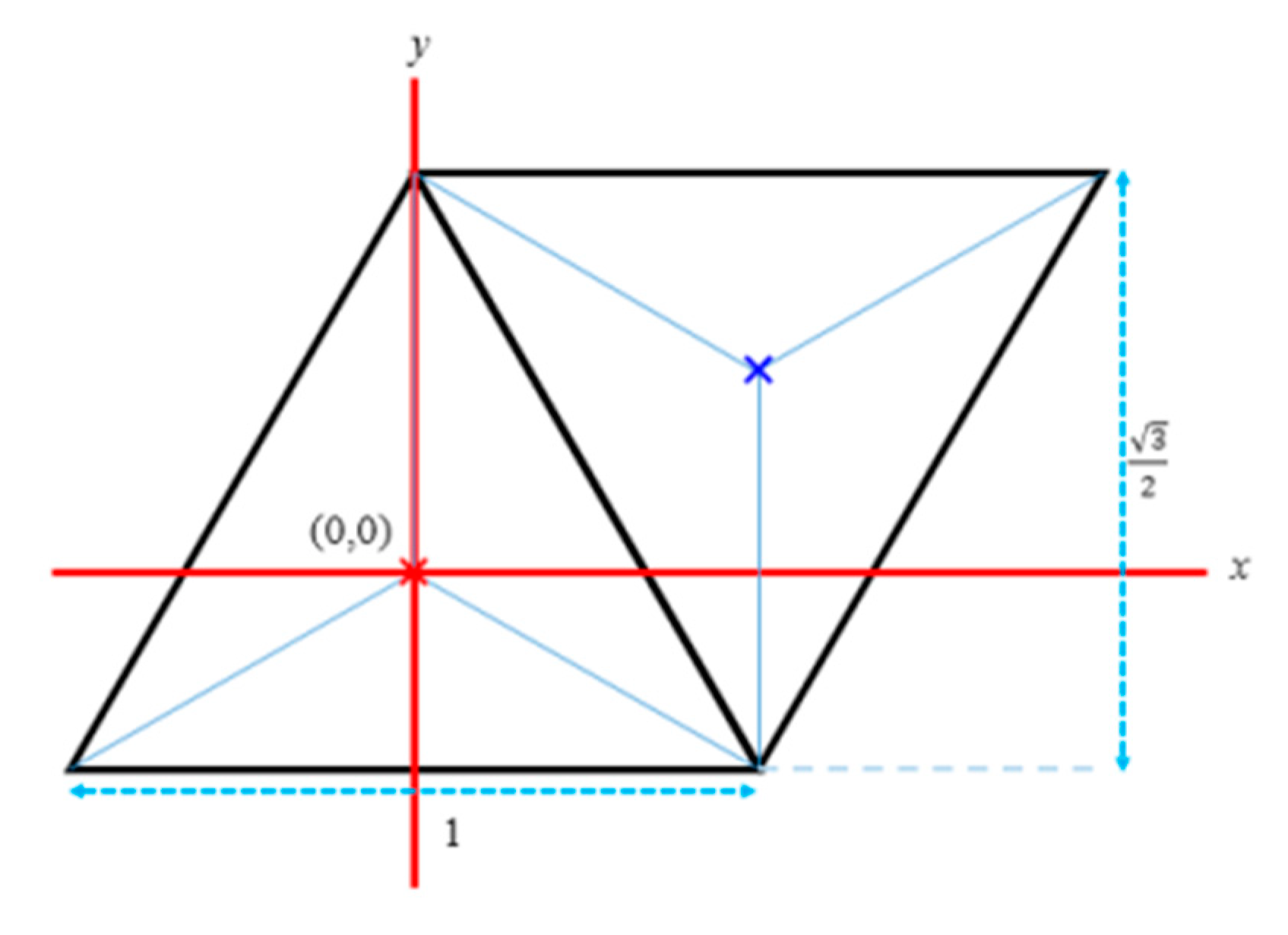
2.2. Notions and Notations on the Triangular Grid

In order to begin the scientific part on the triangular grid, some basic measures of triangles of the grid must be given. Accordingly, as can be seen in Figure 3, the side-length of each triangle is set to 1, and consequently, their height is $\sqrt{3}/2.$ The origin is the midpoint of a Δ oriented triangle. The two marked points in Figure 3 are representing the midpoints of the triangles: The red point is the midpoint of the even triangle, and the blue point is the midpoint of the odd one. The names “even” and “odd” triangles are referring to the orientations of the triangles that are Δ and $\nabla$, respectively. Notice that the closest neighbors of an even triangle are odd ones, and vice versa. Further, we simply use the term “neighbors” for closest neighbors.

The sets of the odd and even triangles (their midpoints) of the triangular grid can be described in the Cartesian coordinate system by the two sets defined in Equations (1) and (2), respectively.

$$O=\left\{\left(a,b\right)|a=\frac{m+1}{2},b=\frac{\sqrt{3}\left(3n-2\right)}{6},m,n\in \mathbb{Z}, m+n\mathrm{is}\mathrm{odd}\right\}$$

(1)

$$E=\left\{\left(a,b\right)|a=\frac{m}{2}, b=\frac{n\sqrt{3}}{2},m,n\in \mathbb{Z}, m+n \mathrm{is}\mathrm{even}\right\}$$

(2)

In the next section, we present some technical details, and then in Section 4 we show our main results.

3. Translations on the Triangular Grid

Opposite to the square grid, the translations on the triangular grid could be bijective or non-bijective, therefore, these concepts will be investigated and characterized in detail in the next sections. Now we present digitized translations in a formal way.

Let G denote the set of coordinate pairs of the digital plane corresponding to the midpoints of the triangle pixels. Let $\tau$ be a translation on G by an arbitrary 2D vector. Generally, $\tau \left(G\right)⊈G$. Therefore to define digitized translation that maps $\tau \left(G\right)$ to G, the result of $\tau \left(G\right)$ is combined with the digitization operation D. $D: \tau \left(G\right)\to G.$

Thus, digitized translation is defined as $D_{\tau }=D\circ \tau \left(G\right)$ as usual.

Definition 1.

Let$D_{\tau }$be a digitized translation and let$i\in G$be the midpoint of a triangular pixel. Then the set of preimages of i with respect to$D_{\tau }$is defined as$P\left(i\right)=\left\{x\in G|D_{\tau }\left(x\right)=i\right\}.$

In the triangular grid G, $\left|P\left(i\right)\right|\in \left\{0,1,2\right\}$, points q and p can be preimages of the same point i only if the distance between q and p is $\sqrt{3}/3.$ The non-injective (not one-to-one) and non-surjective (not onto) digitized translations occur when P(i) = 2 or 0 for some point i, respectively.

Accordingly, a non-bijective translation in the triangular grid would happen when two distinct points have the same image or no images at all correspond to a pixel (see Figure 4, right). As one can observe in the figure, we have both bijective and non-bijective translations on the triangular grid depending on the value of the translation vector.

It is worth saying that a translation in the triangular grid that leads to an injective case will concurrently lead to a surjective one and vice versa. Therefore, having or missing one of those properties will automatically lead to having or missing the other. Thus, non-bijective translations are not injective and not surjective on the triangular grid.

In order to make our study easier and to give more comprehensive descriptions of the translations on the triangular grid, we need to examine some properties of the translation vectors.

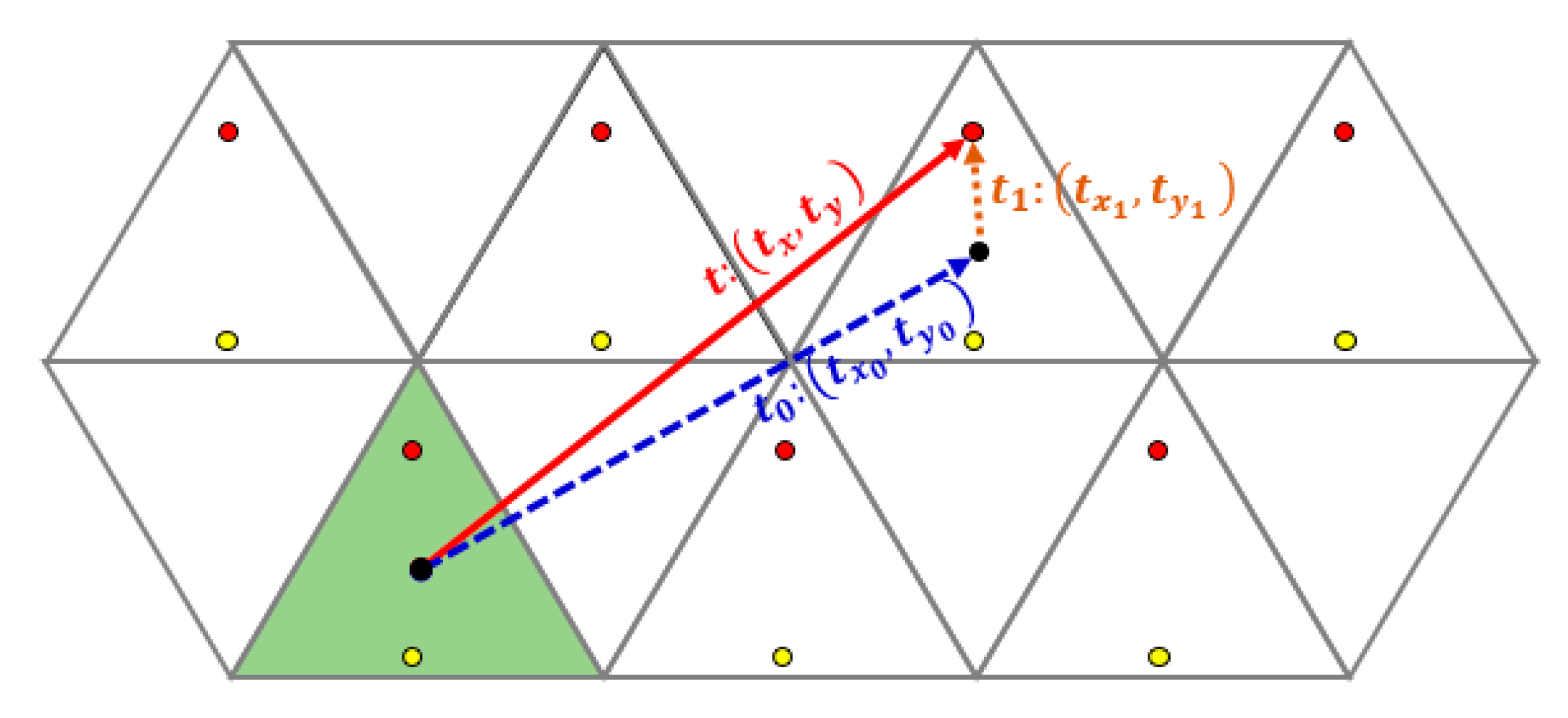
3.1. “Integer” + “Fractional” Vectors

For any translation vector t(t_x, t_y)$\in$ ${ℝ}^2$, we draw it and consider it in a way that we fix its starting point to the grid origin, which is an even midpoint. Then, moreover, we write t as a sum of two vectors, the so-called integer and fractional vectors making some analogy to the traditional grid case. The integer vector will start at the grid origin and end at the closest even midpoint (technical details about this are discussed in the next subsection) to the endpoint of the original translation vector t. On the other hand, the fractional vector will start from the endpoint of the integer vector and end at the endpoint of the original translation vector t, and t₁ is the “fractional” vector.

For illustration, consider Figure 5, where t is the original translation vector and t₀ = $\left(t_{x_0},t_{y_0}\right),$ shown with the longer broken arrow is the integer translation vector which has its endpoint at the nearest even midpoint to the endpoint of t. While t₁, the other broken arrow in the figure, represents the fractional vector that starts at the endpoint of t₀ and ends at the endpoint of t. We can write the translation vector t as: $\left(t_x,t_y\right)=\left(t_{x_0},t_{y_0}\right)+\left(t_{x_1},t_{y_1}\right)$, where $\left(t_{x_0},t_{y_0}\right)$ is the integer part of the translation vector and $\left(t_{x_1},t_{y_1}\right)$ is the fractional part of the translation vector. The integer vector maps the grid into itself. Consequently, the fractional part of the translation vector, t₁, would give the same type (i.e., bijective or not) of translation as the original translation vector t would give.

Therefore, from now on, instead of any translation vectors, we will analyze mainly its fractional part t₁ (see Figure 5).

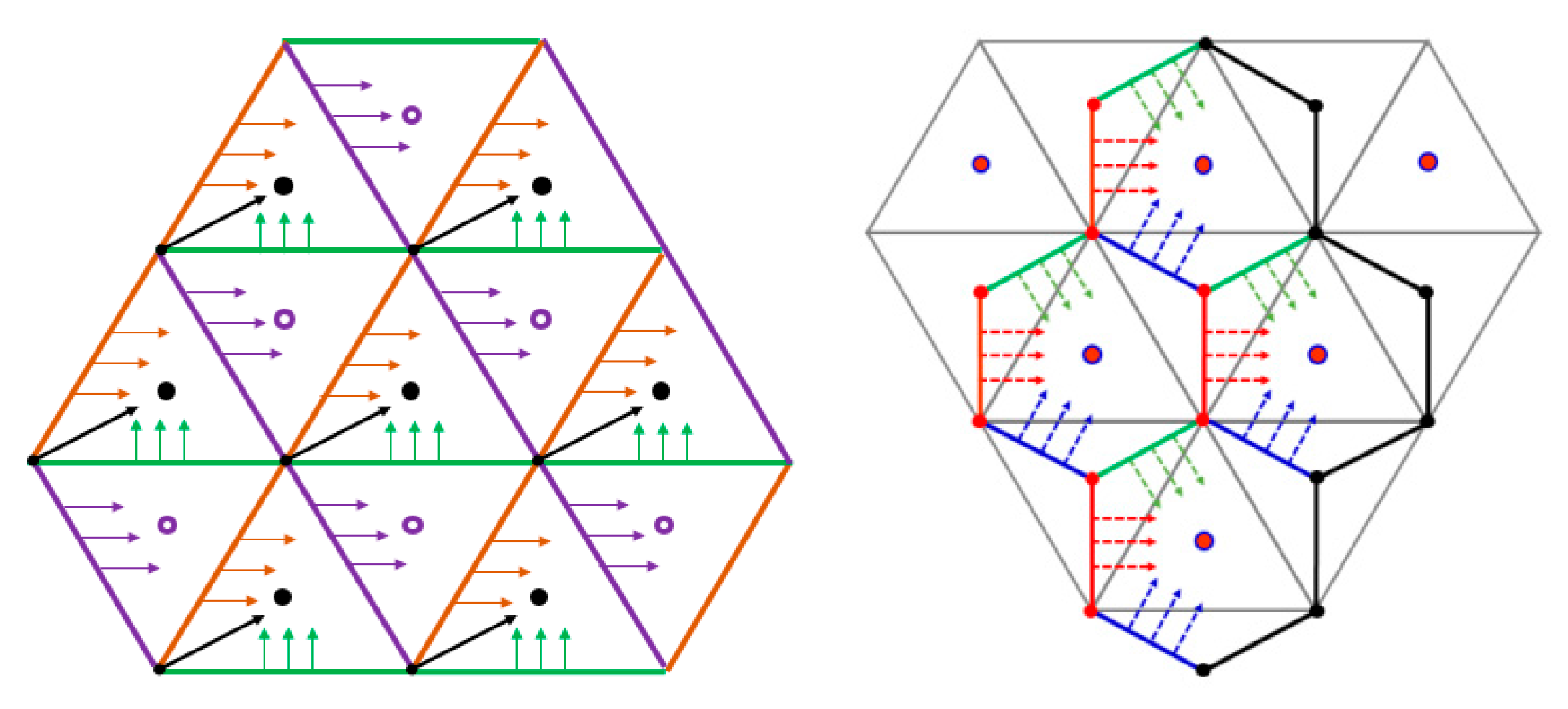
3.2. Rounding the Border Points

In the previous section, it was written that we use the closest midpoint of an even pixel, however, geometrically, it may not be a uniquely defined point. Therefore, in this subsection, we will describe and discuss mapping (rounding) the points of the plane to their closest midpoints. Especially those points that are on the borders of the triangle pixels are of interest. Obviously, the points which are not on the border could be rounded simply to its nearest midpoint based on measuring the shortest distance. Opposite to this, for the points on the border, we have to make some decision to force a unique solution. We round them based on the technique shown also in Figure 6 and detailed below.

Let the borders of triangles take three different colors as in Figure 6 (left), purple (direction ‘\’ with slope $-\sqrt{3}$), brown (direction ‘/’ with slope $\sqrt{3}$), and the green (horizontal) border lines. The next points are listing the cases where a point on the border could be.

(1) The corners of the triangles, the crossing points of these colored lines, have coordinates given in Equation (3).

$$\mathrm{C}=\left\{\left(x,y\right) | x=\frac{m}{2}, y=\frac{\sqrt{3}\left(3n+2\right)}{6}, m,n\in \mathbb{Z}, m+n \mathrm{is}\mathrm{even}\right\}$$

(3)

Further, a point having a coordinate pair (x, y) is lying on one of these borders in the following cases.

(2) Let (a, b) be the closest even midpoint (the midpoint of the even triangle) for (x, y). The point (x, y) lies on a ‘/’ direction, brown line (in Figure 6, left) if

$$\sqrt{3}·\left(x-a+\frac{1}{3}\right)+b=y.$$

(4)

(3) The point (x, y) lies on a ‘\’ direction, purple line if

$$\sqrt{3}·\left(a-x+\frac{1}{3}\right)+b=y.$$

(5)

(4) The point (x, y) lies on a ‘—’ direction, i.e., horizontal, green border line if

$$b - \frac{\sqrt{3}}{6}=y.$$

(6)

Now, let us show the decision in which the pixel (midpoint) is assigned to the points.

(1)

Every corner point is mapped to the nearest even midpoint which has the maximal x coordinate value among the pixels sharing this corner point.

(2)

For points which are not corner points, we have the following strategy:

(3)

Every non-corner point on the ‘/’ direction (brown) border lines is mapped to the nearest even midpoint.

(4)

Every non-corner point on the ‘\’ direction (purple) border lines is mapped to the nearest odd midpoint.

(5)

Every point on the horizontal (green) border lines that is not a corner is mapped to the nearest even midpoint.

(6)

For the sake of completeness, we also give the assignment for all other points:

(7)

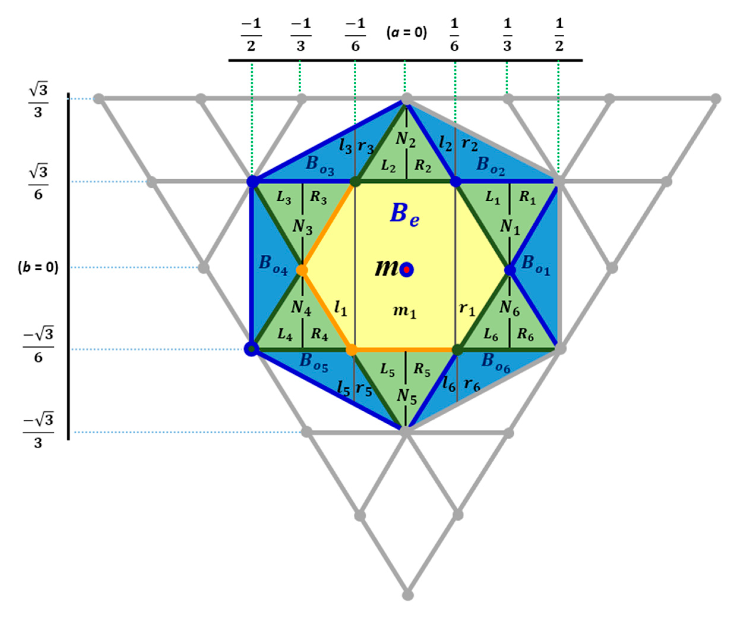
Finally, every point (x, y) which is not on the borders should be mapped to its nearest midpoint based on their distances.

Figure 6 (left) summarizes the assigned triangles for the points on the border shared by more than one triangle pixel.

Finally, in a similar manner, we also assign the closest even midpoint to any point of the plane in a unique way. For points equidistant from more even midpoints, Figure 6 (right) shows the assigned even midpoint.

4. Main Results: Characterizing Strongly Bijective, Semi-Bijective, and Non-Bijective Translation Vectors

As we have fixed the beginning of the translation vectors to the midpoint of an even triangle (let us say, to the origin), we can characterize the vectors by the position of their endpoints. Remember, that by using an integer translation vector, the grid is mapped exactly to itself [4], thus we are interested to analyze only the possible fractional parts of the translation vectors. In our description, we use various regions meaning that if the endpoint of the fractional vector lies in the given region, then the translation with the given vector has some specific property. In the next subsections, we give our main results by characterizing bijective and non-bijective translations. Moreover, we show two different types of bijective translations.

In the following subsections, we detail the properties of the translations based on the fractional part of their vector. We are willing to show that in Figure 7 the shaded regions represent the translations with the following property: The translation is a non-bijective translation if and only if the fractional part of the translation vector ends in the regions N_i (green) where i = 1…6; whereas the translation is bijective if and only if the fractional part of the translation vector ends in any of B_e (the yellow) or $B_{o_i}$ (the blue) regions. There is no other case. Therefore, translation by a specific vector (see, e.g., the red arrows in Figure 4) would lead to bijective transformation (e.g., Figure 4, left) or non-bijective transformation (e.g., Figure 4, right) based on the position of its endpoint.

4.1. Vectors of Bijective Translations

First, the bijective translations are considered. Let us analyze translation vectors with the fractional part ending in the B regions. There are two groups of B regions: B_e and B_o based on their locations in the even triangle Δ, or in an odd triangle $\nabla$, respectively. These bijective translation regions are described as follows. In an even triangle, consider a regular hexagon B_e with a side length of $1/3$ and its center point is the even midpoint. While in the odd triangles, consider the six obtuse-angled triangles $B_{o_i}$ (i = 1…6) as shown in Figure 7. Instead of proving the bijectivity of these cases with common proof here, we show that the two types of regions, although in both cases the translations are bijective, have very different behavior. We define and differentiate strongly and semi-bijective translations:

Definition 2.

Let a be the midpoint of a triangle and a_i be the midpoint of its neighbors where i = 1…3. Let a and a_i be mapped to$D_{\tau }$(a) and $D_{\tau }$(a_i), respectively (where $D_{\tau }$(a) and$D_{\tau }$(a_i) are the digitized translated midpoints of a and its neighbors a_i). If the neighbor relations between a and a_i are kept preserved after the translation, i.e., if $D_{\tau }$(a) and $D_{\tau }$(a_i) are also neighbors for each i = 1…3, then the translation is strongly bijective.

Definition 3.

Let a be the midpoint of a triangle and a_i be the midpoints of its neighbors where i = 1…3. Let a and a_i be mapped to$D_{\tau }$(a) and $D_{\tau }$(a_i), respectively. If the translation is bijective, but the neighborhood is not preserved, (i.e., there is a neighbor a_i of a such that $D_{\tau }$(a) and $D_{\tau }$(a_i) are not neighbors), then the translation is called semi-bijective.

More precise descriptions and characterizations of both categories will be given in the next two sub-sections.

4.1.1. Characterizing Strongly Bijective Translations

Proposition 1.

A translation is strongly bijective if and only if it preserves the parity of the points, i.e., the image of an even point is even and the image of an odd point is odd.

It is clear that if an even point is mapped to even point then all even points are mapped to even points, and a similar statement is fulfilled for the odd points. Now let us prove Proposition 1.

Proof. 

If a translation maps even points to even points and odd points to odd points, it is clear that two neighbor points (from which one must be odd and the other must be even) cannot be mapped to the same triangle. Thus the translation is bijective. Moreover, the neighbor relation is obviously also preserved (See, e.g., Figure 8; more explanation is given in the next proposition).

In the other direction, if an even pixel is translated to an odd pixel or an odd pixel is translated to an even pixel, then there are two cases (See e.g., Figure 4 and Figure 10). In the first case, only one type of pixel is mapped to the opposite type of pixel. More precisely: Either even pixels are mapped to odd pixels and also the odd pixels are mapped to odd pixels, or both the even and odd pixels are mapped to even pixels. Clearly, in this case, the translation is not bijective. The second case is when each pixel is mapped to an opposite type pixel. However, in this case, because of the different (i.e., opposite) directions of the neighbors of the different type points, it is easy to find neighbor points such that their images are not neighbors. (More details are shown in the next subsections). □

We continue this subsection by defining formally the region B_e. By Equation (7) we do it as a union of three smaller pairwise disjoint regions. Notice that in some conditions sharp inequality is used, while in some others, equality is also allowed (See Figure 7).

$$\begin{gathered} {\mathit{B}}_{\mathit{e}}=l_1{{\displaystyle \cup }}^{}{m}_1{{\displaystyle \cup }}^{}{r}_1,\mathrm{where} \\ {l}_1= \left\{\left(x,y\right)|a-\frac{1}{3}\le x<a-\frac{1}{6},\sqrt{3}\left(a-x-\frac{1}{3}\right)+b\le y\le \sqrt{3}\left(x-a+\frac{1}{3}\right)+b\right\} \\ {m}_1=\left\{\left(x,y\right)|a-\frac{1}{6}\le x<a+ \frac{1}{6},b-\frac{\sqrt{3}}{6}\le y<b+\frac{\sqrt{3}}{6}\right\} \\ {r}_1= \left\{\left(x,y\right)|a+\frac{1}{6}\le x\le a+\frac{1}{3}, \sqrt{3}\left(x-a-\frac{1}{3}\right)+b<y<\sqrt{3}\left(a-x+\frac{1}{3}\right)+b\right\} \end{gathered}$$

(7)

Theorem 1.

A translation with vector t = (t_x, t_y) is strongly bijective if and only if$\left(t_{x_1},t_{y_1}\right)$ends at the region B_e, where$\left(t_x, t_y\right) = \left(t_{x_0},t_{y_0}\right) + \left(t_{x_1},t_{y_1}\right)$with integer vector$\left(t_{x_0},t_{y_0}\right)$and fractional vector t₁ =$\left(t_{x_1},t_{y_1}\right).$

Proof. 

Based on Proposition 1, we need to prove that translation with the fractional vector belonging to region B_e preserves the parity of the pixels. Without loss of generality, consider B_e (the yellow) and ${\mathit{B}}_{\mathit{e}}^{\mathbf{\prime }}$ (the blue) isometric regular hexagons within the area of the even and odd triangles, respectively, in Figure 8. Here, m (the red) and n (the yellow) points are the midpoints of the even and odd triangles, respectively.

If t is a translation vector with fractional part t₁ in B_e, then the midpoint of an even pixel m (e.g., the red point) is translated into region B_e around a midpoint of an even pixel as it is shown in Figure 8. By our rounding operator, one can see that the parity of each even pixel is preserved; the points in B_e belong to an even triangle.

On the other hand, the translation of an odd pixel by a vector with fractional part t₁ in B_e implies that the midpoint of the odd pixel n (e.g., the yellow point) is translated to a point belonging to region ${\mathit{B}}_{\mathit{e}}^{\mathbf{\prime }}$ (Figure 8). However, by the rounding operator, it is clear that these points are mapped to n (the yellow point), i.e., to the midpoint of an odd pixel. Therefore, the parity of the original pixel is exactly the same as the parity of its image after the translation. The proof is finished. □

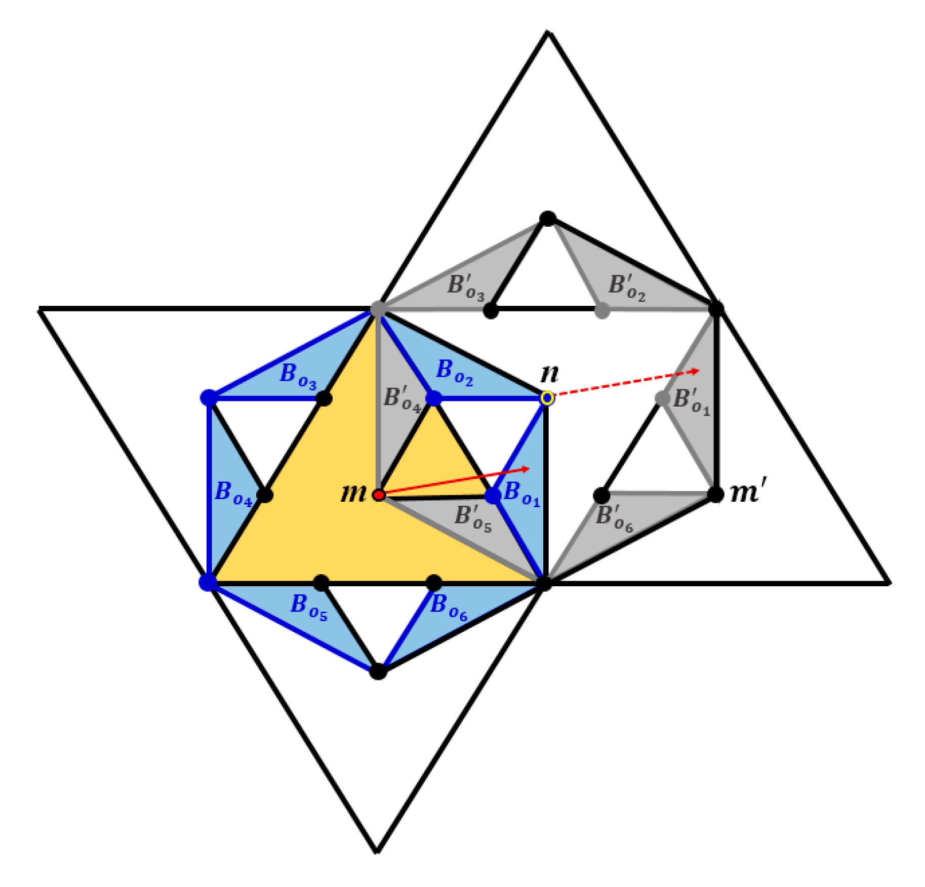
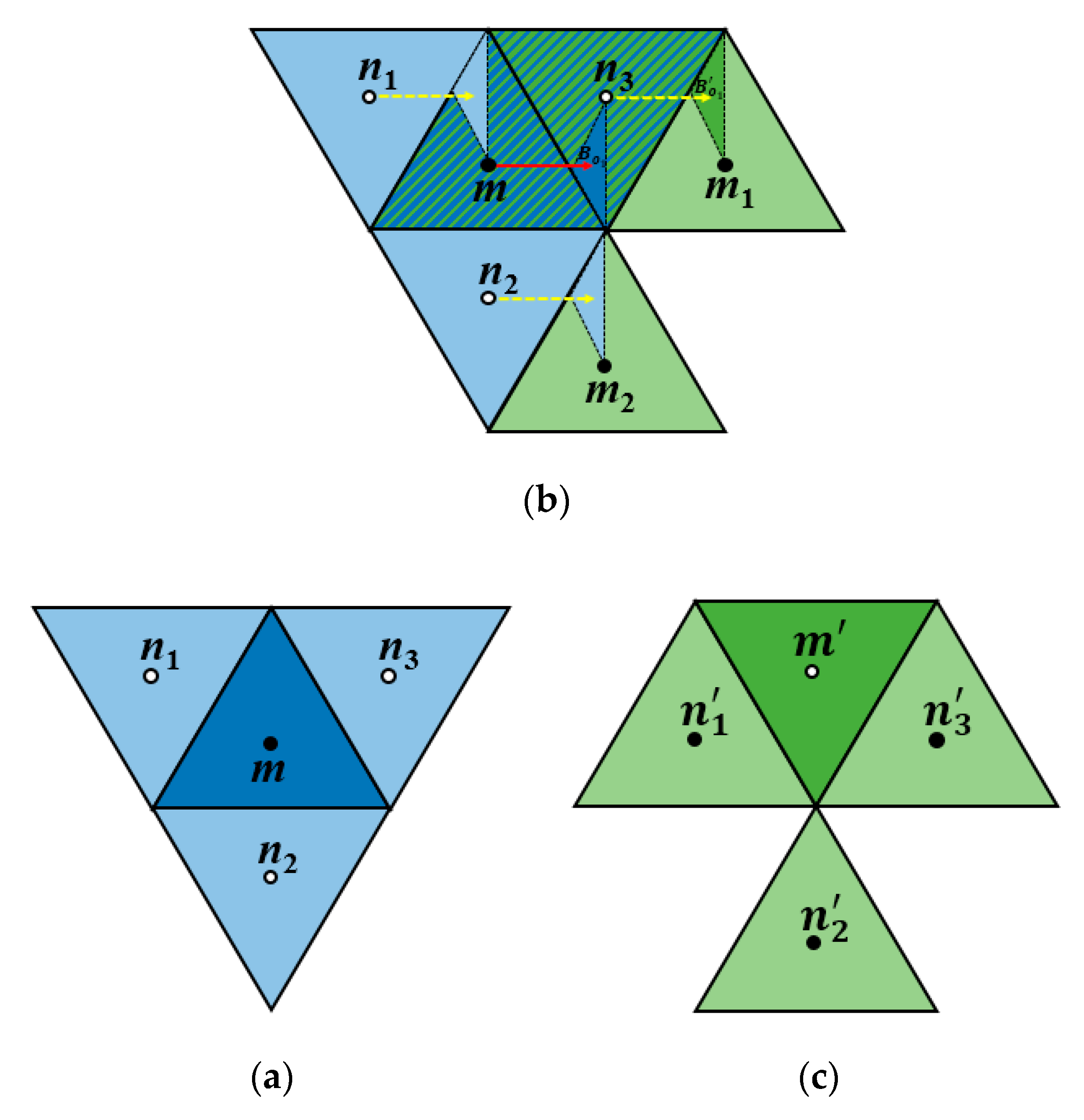
4.1.2. Characterizing Semi-Bijective Translations

We start this subsection by describing the regions where the fractional part of the translation vector is ending in this case, then we formally state our results.

The regions named $B_{o_i}$ (where i = 1…6) in Figure 7 are described by sets defined in Equations (8)–(13). As we will show, these regions represent the semi-bijective translations. Notice that in some conditions sharp equality and inequality are used to deal correctly with the border points.

$${\mathit{B}}_{{\mathit{o}}_{\mathbf{1}}}=\left\{\left(x,y\right)|a+\frac{1}{3}\le x<a+\frac{1}{2},\sqrt{3}\left(a-x+\frac{1}{3}\right)+b\le y\le \sqrt{3}\left(x-a-\frac{1}{3}\right)+b\right\}$$

(8)

$$\begin{gathered} {\mathit{B}}_{{\mathit{o}}_{\mathbf{2}}}=l_2{{\displaystyle \cup }}^{}{r}_2\mathrm{where} \\ l_2=\left\{\left(x,y\right)| a<x<a+\frac{1}{6}, \sqrt{3} \left(a-x+\frac{1}{3}\right)+b\le y<\frac{\sqrt{3}}{3}\left(a-x+1\right)+b\right\} \\ r_2=\left\{\left(x,y\right)|a+\frac{1}{6}\le x\le a+\frac{1}{2},b+\frac{\sqrt{3}}{6}\le y<\frac{\sqrt{3}}{3}\left(a-x+1\right)+b\right\} \end{gathered}$$

(9)

$$\begin{gathered} {\mathit{B}}_{{\mathit{o}}_{\mathbf{3}}}=l_3{{\displaystyle \cup }}^{}{r}_3\mathrm{where} \\ l_3=\left\{\left(x,y\right)|a-\frac{1}{2}\le x<a-\frac{1}{6},b+\frac{\sqrt{3}}{6}\le y\le \frac{\sqrt{3}}{3}\left(x- a+1\right)+b\right\} \\ r_3=\left\{\left(x,y\right)|a-\frac{1}{6}<x<a,\sqrt{3}\left(x-a+\frac{1}{3}\right)+b<y\le \frac{\sqrt{3}}{3}\left(x- a+1\right)+b\right\} \end{gathered}$$

(10)

$${\mathit{B}}_{{\mathit{o}}_{\mathbf{4}}}=\left\{\left(x,y\right)|a-\frac{1}{2}\le x\le a-\frac{1}{3}, \sqrt{3}\left(x-a+\frac{1}{3}\right)+b<y<\sqrt{3}\left(a-x-\frac{1}{3}\right)+b\right\}$$

(11)

$$\begin{gathered} {\mathit{B}}_{{\mathit{o}}_{\mathbf{5}}}=l_5{{\displaystyle \cup }}^{}{r}_5\mathrm{where} \\ l_5=\left\{\left(x,y\right)| a-\frac{1}{2}<x\le a-\frac{1}{6},\frac{\sqrt{3}}{3} \left(a-x-1\right)+b\le y<b-\frac{\sqrt{3}}{6}\right\} \\ r_5=\left\{\left(x,y\right)|a-\frac{1}{6}\le x\le a,\frac{\sqrt{3}}{3} \left(a-x-1\right)+b\le y<\sqrt{3}\left(a-x-\frac{1}{3}\right)+b\right\} \end{gathered}$$

(12)

$$\begin{gathered} {\mathit{B}}_{{\mathit{o}}_{\mathbf{6}}}=l_6{{\displaystyle \cup }}^{}{r}_6\mathrm{where} \\ l_6=\left\{\left(x,y\right)| a\le x<a+\frac{1}{6},\frac{\sqrt{3}}{3} \left(x-a-1\right)+b\le y<\sqrt{3}\left(x-a-\frac{1}{3}\right)+b\right\} \\ r_6=\left\{\left(x,y\right)|a+\frac{1}{6}<x<a+\frac{1}{2},\frac{\sqrt{3}}{3} \left(x-a-1\right)+b\le y<b-\frac{\sqrt{3}}{6}\right\} \end{gathered}$$

(13)

Now we state and prove that any translation with a fractional vector belonging to a region $B_{o_i}$ switches the parity of the pixels.

Proposition 2.

A translation with vector t = (t_x, t_y) = t₀ + t₁ is mapping every pixel to an opposite type pixel if and only if the fractional vector t₁ =$\left(t_{x_1},t_{y_1}\right)$ends in a region$B_{o_i}$where i = 1…6.

Proof. 

Let us consider the isometric obtuse-angled isosceles triangles ${\mathit{B}}_{{\mathit{o}}_{\mathbf{1}}}$ and ${\mathit{B}}_{{\mathit{o}}_{\mathbf{1}}}^{\mathbf{\prime }}$ within the area of the odd and even triangles, respectively, in Figure 9. Let m (the red point in Figure 9) denote the midpoint of the corresponding even triangle and n (the yellow point) denote the midpoint of the odd triangle, respectively. If t is a translation vector with fractional part t₁ belonging to region ${\mathit{B}}_{{\mathit{o}}_{\mathbf{1}}}$, then the midpoint of an even pixel m (e.g., the red point) is translated into region ${\mathit{B}}_{{\mathit{o}}_{\mathbf{1}}}$ inside an odd pixel as it is shown in Figure 9. By our rounding operator, one can see that the parity of each even pixel is changed to odd; the points in ${\mathit{B}}_{{\mathit{o}}_{\mathbf{1}}}$ belong to an odd triangle. On the other hand, the translation of an odd pixel by a vector with fractional part t₁ belonging to ${\mathit{B}}_{{\mathit{o}}_{\mathbf{1}}}$ implies that the midpoint of the odd pixel n (e.g., the yellow point) is translated to a point belonging to region ${\mathit{B}}_{{\mathit{o}}_{\mathbf{1}}}^{\mathbf{\prime }}$ (Figure 9). However, by applying the rounding operator on the edges, it is clear that these points are mapped to the midpoint of an even pixel ($m^{\prime }$). Therefore, the parity of the original pixel is opposite to the parity of its image after the translation.

Having the even midpoint (m) translated to ${\mathit{B}}_{{\mathit{o}}_{\mathbf{2}}},{\mathit{B}}_{{\mathit{o}}_{\mathbf{3}}},$${\mathit{B}}_{{\mathit{o}}_{\mathbf{4}}},{\mathit{B}}_{{\mathit{o}}_{\mathbf{5}}},\mathrm{and} {\mathit{B}}_{{\mathit{o}}_{\mathbf{6}}}$ (Figure 9) the proof goes in a similar manner. □

Theorem 2.

A translation with vector t = (t_x, t_y) = t₀ + t₁ is a semi-bijective mapping if and only if the fractional vector t₁ =$\left(t_{x_1},t_{y_1}\right)$ends in a region$B_{o_i}$where i = 1…6.

Proof. 

We have already shown that translations that preserve the parity of the pixels are strongly bijective. It is clear, that if an even point is mapped to an even point, then all even points are mapped to even points, and if an even point is mapped to an odd point then all even points are mapped to odd points. If both even and odd points are mapped to the same type of points, then the translation is not bijective, since no point will be mapped to the other type of point. What remains to show is that if odd points are translated to even points and even points are translated to odd points, then the neighborhood structure is lost by the translation. Let us consider, first, the regions ${\mathit{B}}_{{\mathit{o}}_{\mathbf{1}}}$ and ${\mathit{B}}_{{\mathit{o}}_{\mathbf{1}}}^{\mathbf{\prime }}$. As one can observe in Figure 10, the neighbors of a pixel are not mapped to the neighbors of the pixel obtained by the translation.

The proof goes analogously for the other five regions. □

Summarizing the cases of bijective translations, the B_e (the yellow) region refers to the strongly bijective transitions, while $B_{o_i}$ where i = 1…6, (the blue) regions specify the semi-bijective translations (in Figure 7). Based on Proposition 2 and Theorem 2, we can say that a translation is semi-bijective if and only if it is a bijective translation and it maps the elements of O (i.e., the odd points) to E (i.e., even points) and vice versa.

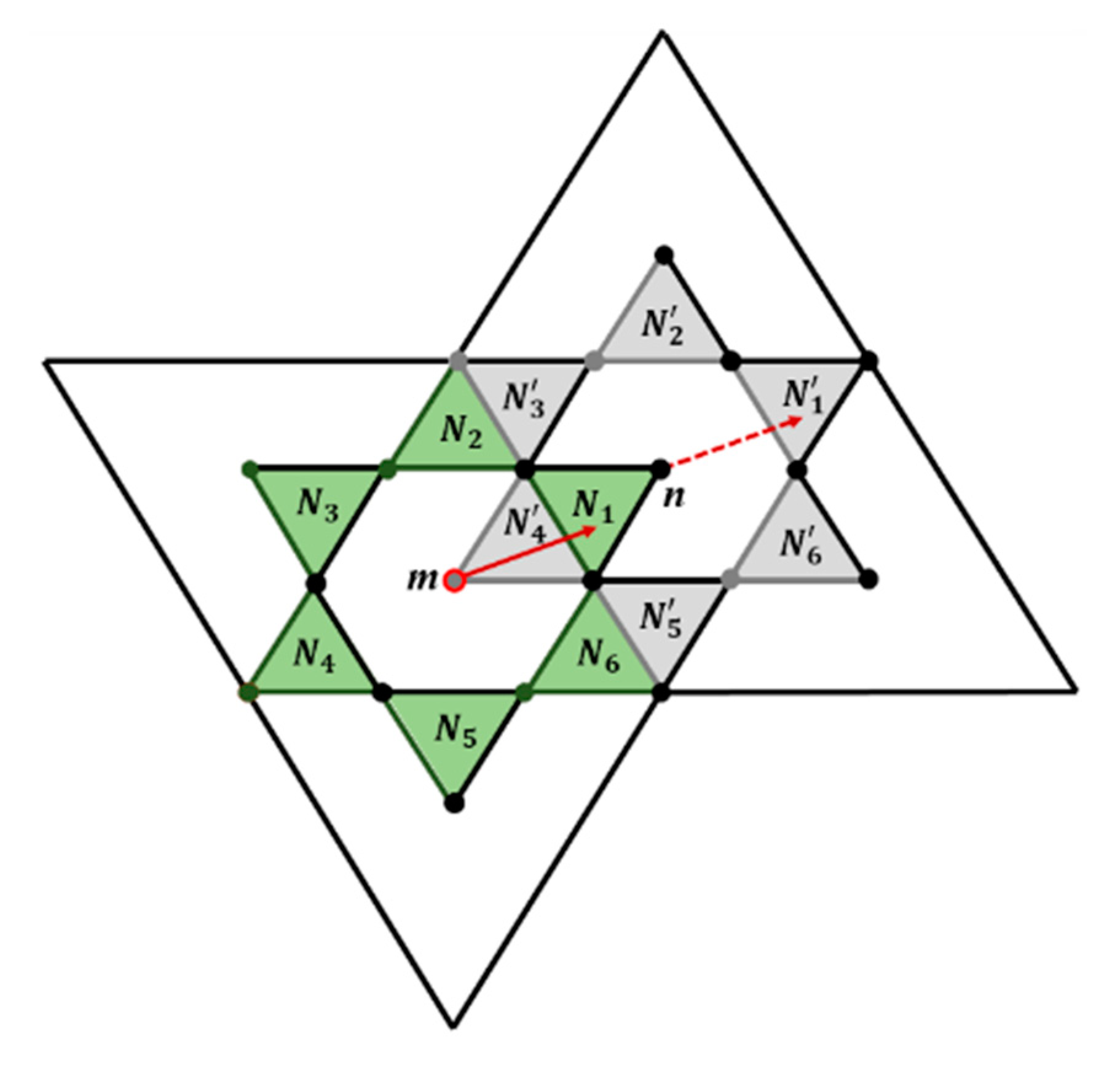
4.2. Characterizing the Non-Bijective Translation Vectors

Proposition 3.

A translation is non-bijective if and only if it maps all the pixels (both E and O) to exactly one of the sets O or E.

Proof. 

Obviously, translations are not bijective if only one of the sets O and E is used as the image of the translation. On the other hand, all translations must satisfy the condition of exactly one of Propositions 1, 2 or 3, thus the statement of this proposition is proven. □

At translations having vectors with fractional parts ending in the regions N_i where i = 1…6 (the green regions in Figure 7), points without pre-image (holes) and also points with two pre-images occur. Hence, these are non-bijective translations (see Figure 4, right, for an example).

Now, in order to describe these non-bijective translations mathematically, the six equilateral triangles N_i where i = 1…6 (the green regions in Figure 7), will be categorized into two groups. The odd and even groups are based on the base odd $\nabla$ and even Δ triangles in which these green triangles are located. Remember that the translation vectors in our description start at the midpoint of an even triangle (e.g., the origin), and we deal with its fractional part.

There are three green regions N_i in each odd and even triangle, they are denoted by N₁, N₃, and N₅ for the odd triangle, and N₂, N₄, and N₆ for the even triangle (as Figure 7 shows both cases). To simplify their mathematical description, each of them is split into two symmetrical parts L_i and R_i, where i = 1…6, as their left and right parts (Figure 7). Equations (14)–(19) describe them as follows. Let (a, b) denote the coordinate pair of the midpoint of the even pixel from where the fractional vector starts (denoted by the red circle in Figure 7).

$$\begin{gathered} {\mathit{N}}_{\mathbf{1}}=L_1{{\displaystyle \cup }}^{}{R}_1\mathrm{where} \\ L_1=\left\{\left(x,y\right) |a+\frac{1}{6}\le x\le a+\frac{1}{3},\sqrt{3}\left(a-x+\frac{1}{3}\right)+b<y\le b+\frac{\sqrt{3}}{6} \right\} \\ R_1=\left\{\left(x,y\right) |a+\frac{1}{3}<x\le a+\frac{1}{2},\sqrt{3}\left(x-a-\frac{1}{3}\right)+b\le y\le b+\frac{\sqrt{3}}{6}\right\} \end{gathered}$$

(14)

$$\begin{gathered} {\mathit{N}}_{\mathbf{2}}=L_2{{\displaystyle \cup }}^{}{R}_2\mathrm{where} \\ L_2=\left\{\left(x,y\right)|a-\frac{1}{6}<x<a, b+\frac{\sqrt{3}}{6}<y<\sqrt{3}\left(x-a+\frac{1}{3}\right)+b\right\} \\ R_2=\left\{\left(x,y\right)|a\le x\le a+\frac{1}{6},b+\frac{\sqrt{3}}{6}<y<\sqrt{3}\left(a-x+\frac{1}{3}\right)+b\right\} \end{gathered}$$

(15)

$$\begin{gathered} {\mathit{N}}_{\mathbf{3}}=L_3{{\displaystyle \cup }}^{}{R}_3\mathrm{where} \\ L_3= \left\{\left(x,y\right) |a-\frac{1}{2}\le x\le a-\frac{1}{3},\sqrt{3}\left(a-x-\frac{1}{3}\right)+b<y\le b+\frac{\sqrt{3}}{6}\right\} \\ R_3= \left\{\left(x,y\right)|a-\frac{1}{3}<x<a-\frac{1}{6},\sqrt{3}\left(x-a+\frac{1}{3}\right)+b\le y\le b+\frac{\sqrt{3}}{6}\right\} \end{gathered}$$

(16)

$$\begin{gathered} {\mathit{N}}_{\mathbf{4}}=L_4{{\displaystyle \cup }}^{}{R}_4\mathrm{where} \\ L_4=\left\{\left(x,y\right)|a-\frac{1}{2}<x\le a-\frac{1}{3},b-\frac{\sqrt{3}}{6}<y<\sqrt{3}\left(x-a+\frac{1}{3}\right)+b\right\} \\ R_4=\left\{\left(x,y\right)|a-\frac{1}{3}<x\le a-\frac{1}{6},b-\frac{\sqrt{3}}{6}<y\le \sqrt{3}\left(a-x-\frac{1}{3}\right)+b\right\} \end{gathered}$$

(17)

$$\begin{gathered} {\mathit{N}}_{\mathbf{5}}=L_5{{\displaystyle \cup }}^{}{R}_5\mathrm{where} \\ L_5=\left\{\left(x,y\right) |a-\frac{1}{6}\le x\le a,\sqrt{3}\left(a-x-\frac{1}{3}\right)+b<y\le b-\frac{\sqrt{3}}{6}\right\} \\ R_5=\left\{\left(x,y\right) |a<x<a+\frac{1}{6},\sqrt{3}\left(x-a-\frac{1}{3}\right)+b\le y\le b-\frac{\sqrt{3}}{6}\right\} \end{gathered}$$

(18)

$$\begin{gathered} {\mathit{N}}_{\mathbf{6}}=L_6{{\displaystyle \cup }}^{}{R}_6\mathrm{where} \\ L_6=\left\{\left(x,y\right)|a+\frac{1}{6}<x\le a+\frac{1}{3}, b-\frac{\sqrt{3}}{6}<y<\sqrt{3}\left(x-a-\frac{1}{3}\right)+b\right\} \\ R_6=\left\{\left(x,y\right)|a+\frac{1}{3}<x<a+\frac{1}{2},b-\frac{\sqrt{3}}{6}<y\le \sqrt{3}\left(a-x+\frac{1}{3}\right)+b\right\} \end{gathered}$$

(19)

Theorem 3.

A translation with vector t(x, y) is a non-bijective mapping if and only if t(x, y) = t₀(x₀, y₀) + t₁(x₁, y₁) where t₀ is the integer vector and t₁ is the fractional vector of the translation such that this latter one starts at the endpoint of t₀ and ends at a region N_i where i = 1…6.

Proof. 

Based on Proposition 3, we need to prove that translation with fractional vector t₁ belonging to region N_i where i = 1…6, will map every pixel to the same type of pixel. Without loss of generality, consider the regions N₁ (green) and ${\mathit{N}}_{\mathbf{1}}^{\mathbf{\prime }}$ (gray) in Figure 11. They are, in fact, isometric regular triangles within the area of an odd triangle. Points m (red) and n (yellow) denote the midpoints of the corresponding even and odd triangles, respectively.

If t is a translation vector with fractional part t₁ in N₁, then the midpoint of an even pixel (e.g., the red point m) is translated into the region N₁ around n; the midpoint of an odd pixel as it is shown in Figure 11. By our rounding operator, one can see that the parity of each even pixel is not preserved since the points in N₁ belong to an odd triangle. On the other hand, the translation of an odd pixel by a vector t with fractional part t₁ in N₁ implies that the midpoint of the odd pixel n (e.g., the yellow point in Figure 11) is translated to a point belonging to region ${\mathit{N}}_{\mathbf{1}}^{\mathbf{\prime }}$. However, by the rounding operator, it is clear that these points are mapped again to the midpoint of the odd pixel, i.e., point n. Therefore, both even and odd points are mapped to odd points in this case. The proof is similar for other regions, in fact, for regions N₁, N₃, and N₅, the translation maps every pixel to odd and for regions N₂, N₄, and N₆ it maps every point to even pixels. □

5. Conclusions

Transformations of digital images have very frequent applications. The simplest transformations are the isometric ones, including translations, rotations, and mirroring. In this paper, translations on the triangular grid are investigated and analyzed. Translations are applied in various digital scenarios, e.g., by “drag and drop” for some icons on the computer/tablet/smartphone screen. Although these geometrical transformations are the simplest ones, their discretized versions are not trivial on the triangular grid. As we have seen, since this grid is not a point lattice, some of the discretized translations are not bijective. Thus, one needs to be careful when applying arbitrary translations to images on the triangular grid. We note here that the technique to determine whether a translation is bijective or not is based on the redigitization of the translated image, and thus, it is somewhat similar to [12] and also to the approach counting the number of digitizations of a disk in [13].

It is well known that digital rotations are usually not bijective on any grids, however, the translations are bijective on point lattices. We have discovered various cases of translations on the triangular plane and a full characterization of them is given to three categories. In the future, we plan to analyze also other operations, e.g., rotations [14,15] mixed with translations and other more complex operations on the triangular grid. Our results can be applied not only in image processing and computer graphics, but also, in various engineering solutions connected to digital signal processing, camera sensors, etc. Future work could be to establish connections between various types of translations and visual illusions or image manipulating techniques like dithering.

References

1. Klette, R.; Rosenfeld, A. Digital geometry: Geometric methods for digital picture analysis. In Morgan Kaufmann; Elsevier: San Francisco, CA, USA, 2004; Volume I-XVIII, pp. 1–656. ISBN 978-1-55860-861-0. [Google Scholar]
2. Kaufman, A. Voxels as a computational representation of geometry. Presented at the SIGGRAPH’99—Course 29, Los Angeles Convention Center, Los Angeles, CA, USA, 8–13 August 1999; pp. 14–58. [Google Scholar]
3. Pluta, K.; Romon, P.; Kenmochi, Y.; Passat, N. Bijective Digitized Rigid Motions on Subsets of the Plane. J. Math. Imaging Vis. 2017, 59, 84–105. [Google Scholar] [CrossRef]
4. Nagy, B. Isometric transformations of the dual of the hexagonal lattice. In Proceedings of the 6th IEEE International Symposium on Image and Signal Processing and Analysis, ISPA, Salzburg, Austria, 16–18 September 2009; pp. 432–437. [Google Scholar]
5. Pluta, K.; Romon, P.; Kenmochi, Y.; Passat, N. Bijective rigid motions of the 2D Cartesian grid. In DGCI 2016: Discrete Geometry for Computer Imagery; Lecture Notes in Computer Science; Springer: Cham, Switzerland, 2016; Volume 9647, pp. 359–371. [Google Scholar]
6. Rosenfeld, A. Continuous functions on digital pictures. Pattern Recognit. Lett. 1986, 4, 177–184. [Google Scholar] [CrossRef]
7. Nagy, B. Characterization of digital circles in triangular grid. Pattern Recognit. Lett. 2004, 25, 1231–1242. [Google Scholar] [CrossRef]
8. Nagy, B.; Moisi, E.V. Memetic algorithms for reconstruction of binary images on triangular grids with 3 and 6 projections. Appl. Soft Comput. 2017, 52, 549–565. [Google Scholar] [CrossRef]
9. Kardos, P.; Palágyi, K. Topology preservation on the triangular grid. Ann. Math. Artif. Intell. 2015, 75, 53–68. [Google Scholar] [CrossRef]
10. Kardos, P.; Palágyi, K. Unified Characterization of P-Simple Points in Triangular, Square, and Hexagonal Grids. In Computational Modeling of Objects Presented in Images. Fundamentals, Methods, and Applications, Proceedings of the International Symposium Computational Modeling of Objects Represented in Images, Niagara Falls, NY, USA, 21–23 September 2016; Springer: Cham, Switzerland, 2017; Volume 10149, pp. 79–88. [Google Scholar]
11. Abuhmaidan, K.; Nagy, B. Non-bijective translations on the triangular plane. In Proceedings of the IEEE 16th World Symposium on Applied Machine Intelligence and Informatics (SAMI 2018), Kosice, Slovakia, 7–10 February 2018; pp. 183–188. [Google Scholar]
12. Mazo, L.; Baudrier, É. Object digitization up to a translation. J. Comput. Syst. Sci. 2018, 95, 193–203. [Google Scholar] [CrossRef] [Green Version]
13. Nagy, B. An algorithm to find the number of the digitizations of discs with a fixed radius. Electron. Notes Discret. Math. 2005, 20, 607–622. [Google Scholar] [CrossRef]
14. Avkan, A.; Nagy, B.; Saadetoglu, M. Digitized Rotations of Closest Neighborhood on the Triangular Grid. In Combinatorial Image Analysis, Proceedings of the 19th International Workshop, (IWCIA 2018), Porto, Portugal, 22–24 November 2018; Lecture Notes in Computer Science; Springer: Cham, Switzerland, 2018; Volume 11255, pp. 53–67. [Google Scholar]
15. Avkan, A.; Nagy, B.; Saadetoglu, M. Digitized Rotations of 12 Neighbors on the Triangular Grid. Ann. Math. Artif. Intell. 2019. accepted. [Google Scholar]
Figure 1. The square, hexagonal and triangular grids. Midpoints of the pixels represent their gridpoints. Any grid-vector translates the square and hexagonal grids to themselves, respectively. However, it is not the case in the triangular grid.
Mathematics 08 00029 g001
Figure 2. A translation on the square grid (by the vector represented by the broken arrow). The centers (blue points) represent the original gridpoints, while the red ones are the translated ones. On the right, it is also shown how to deal with points on the edges and on the corners. In the next subsection, some basics of the triangular grid will be recalled.
Mathematics 08 00029 g002
Figure 3. Side-length and height of triangle pixels at the triangular grid. The midpoints of the pixels are also marked. The even midpoint shown is the origin of the grid.
Mathematics 08 00029 g003
Figure 4. A bijective and a non-bijective translation left and right, respectively. The translation vector is shown. In the case of non-bijective translation, two distinct points have the same image and there are pixels that do not correspond to any original pixel.
Mathematics 08 00029 g004
Figure 5. A translation vector t is considered as the sum of two vectors; t0 is the “integer” vector, and t1 is the “fractional” vector.
Mathematics 08 00029 g005
Figure 6. Rounding points of the plane to pixel midpoints (left) and to even midpoints (right).
Mathematics 08 00029 g006
Figure 7. An even pixel with its three closest neighbors. The hexagon region Be (in yellow color) with its orange borders is referred to as the strongly-bijective translation region, whereas the six obtuse-angle triangles B o i where i = 1…6 (in blue color with its dark blue borders) are referred to as the semi-bijective translation regions. The six equilateral triangles N i where i = 1…6 (in green color with its dark green borders) are referred to as the non-bijective translation regions (the starting point of the fractional part of the translation vector is at the even midpoint (m)).
Mathematics 08 00029 g007
Figure 8. Any translation vector that starts at the even midpoint (m) and ends within the hexagonal region (Be) will produce a strongly-bijective translation. The orange- and blue-colored borders belong to Be and B e regions respectively, while the gray-colored borders belong to other regions.
Mathematics 08 00029 g008
Figure 9. Translations with fractional vectors that start at the even midpoint (m) and end at regions B o i (where i = 1…6, the blue colored regions with their dark blue colored borders) will produce semi-bijective translations.
Mathematics 08 00029 g009
Figure 10. (a) An even pixel and its neighbors, the three odd pixels, before translation. (b) A translation by a vector that belongs to the semi-bijective region B o 1 . (c) The result of the translation: m ,   n 1 ,   n 2 ,   and   n 3 are the images of m , n 1 , n 2 ,   and   n 3 respectively. The pixels m and n 2 are not neighbors.
Mathematics 08 00029 g010
Figure 11. A translation to a non-bijective region Ni. Image of an even and of an odd pixel (with the corresponding regions N i . where i = 1…6) is shown.
Mathematics 08 00029 g011