Design and Analysis of a Non-Iterative Estimator for Target Location in Multistatic Sonar Systems with Sensor Position Uncertainties

Abstract

Target location is the basic application of a multistatic sonar system. Determining the position/velocity vector of a target from the related sonar observations is a nonlinear estimation problem. The presence of possible sensor position uncertainties turns this problem into a more challenging hybrid parameter estimation problem. Conventional gradient-based iterative estimators suffer from the problems of initialization difficulties and local convergence. Even if there is no problem with initialization and convergence, a large computational cost is required in most cases. In view of these drawbacks, we develop a computationally efficient non-iterative position/velocity estimator. The main numerical computation involved is the weighted least squares optimization, which makes the estimator computationally efficient. Parameter transformation, model linearization and two-stage processing are exploited to prevent the estimator from iterative computation. Through performance analysis and experimental verification, we find that the proposed estimator reaches the hybrid Cramér–Rao bound and has linear computational complexity.

1. Introduction

In recent years, there has been a lively interest in target location using multistatic sonars [1,2,3,4,5,6,7,8,9,10,11,12,13]. In a multistatic sonar system, the sum of each pair of transmitter–target range and target–receiver range defines an ellipse. Then the target is at the intersection of all these ellipses [7]. The elliptical location encountered in the multistatic sonar systems has also been considered in the MIMO radar [14,15,16,17,18,19,20], multistatic radar [21,22,23,24,25] and indoor positioning systems [26,27].

A considerable amount of literature has been published on the problem of estimating the coordinates of the intersection of the ellipses, which can be statistically modelled as a nonlinear estimation problem. To resolve the essential nonlinearity in the problem, linearization is a natural idea. In particular, the measurement equations were linearized by Taylor expansion, resulting in an iterative algorithm [20]. Alternative to the Taylor expansion, introducing nuisance parameters is another approach to linearization. For example, the classic spherical-interpolation [28] and spherical-intersection [29] methods were ported to the elliptical location problems [25]. However, the estimation accuracy is not optimum in [25]. Slightly more complex than the linear models, a quadratically constrained least squares model was constructed, which is generally difficult to solve effectively [27,30]. More recently, as another major methodology for parameter estimation, a Bayes estimator was presented for elliptical location, involving formidable numerical integration [4]. Intuitively, integrating other kinds of observations helps improve the positioning accuracy. For instance, the Doppler shift measurements were incorporated to improve the position estimate and identify the velocity additionally [5].

In addition to the difficulties raised by the high nonlinearity in the statistical models, another obstacle in the multistatic sonar location is that the complex ocean environments introduce uncertainties in the positions of the transmitters and receivers. Preliminary work considering sensor location errors in elliptical location was reported in the literature [6,10,13]. Recent advances have seen an efficient non-iterative estimator for the multistatic sonar location [5,6] inspired by the renowned work of [31].

Perturbation analysis of least squares problems is a major topic in numerical linear algebra. Related work has focused on establishing various error bounds [32,33,34]. We combine the basic techniques of perturbation analysis with multivariate statistics [35] to quantitatively evaluate the estimators for a nonlinear estimation problem.

On the basis of the above work, our technical contributions are summarized here.

• We establish a statistical model of determining both the position and velocity of a moving target in a multistatic sonar system using differential delays and Doppler shifts. The uncertainties in the sensor positions are carefully taken into account in our model. The performance limit is developed for this problem.
• To tackle the proposed nonlinear hybrid parameter estimation problem, we design an efficient non-iterative solution using parameter transformation, model linearization and two-stage processing.
• We further analyze the bias vector and covariance matrix of our estimator theoretically using the second/first-order perturbation analysis and multivariate statistics.
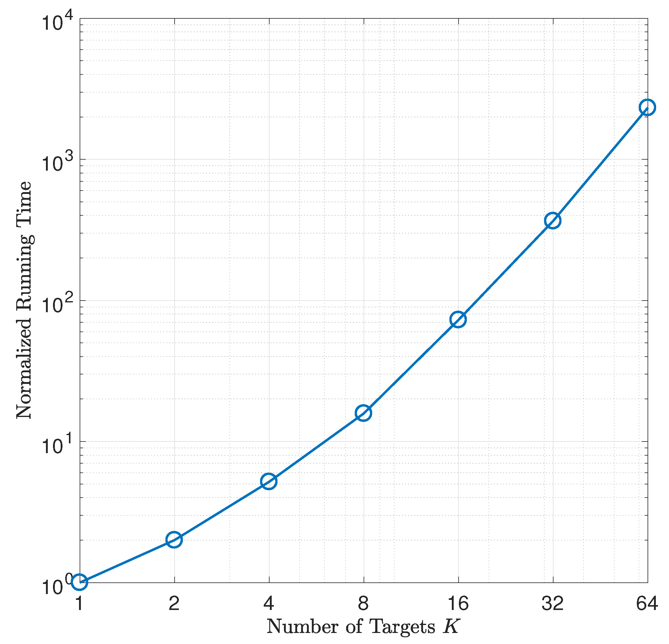
• We prove that the proposed estimator has approximate statistical efficiency and linear complexity.

The rest of this paper is organized as follows. Section 2 lists the notational conventions that will be used throughout the paper. Section 3 provides the location scenario and formulates the problem as a nonlinear estimation problem. In Section 4, we evaluate the performance limit for the proposed problem. Section 5 is devoted to developing our estimator. Then, Section 6 analyzes the bias vector and covariance matrix of our estimator up to the second/first-order random errors. Section 7 contains comprehensive Monte Carlo simulation results, and finally Section 8 draws the conclusion.

2. Notational Conventions

We will use bold lowercase letters to denote the column vectors and bold uppercase ones to denote the matrices. Specifically, ${\mathbf{0}}_{p\times q}$ is a $p\times q$ zeros matrix, ${\mathbf{1}}_{p\times q}$ is a $p\times q$ ones matrix, and $\mathbf{I}$ is an identity matrix of appropriate size. The operators ⊗ and ∘ represent the Kronecker product and Hadamard product respectively. The expression $({\mathbf{M}}_1⪰{\mathbf{M}}_2)$ means that $({\mathbf{M}}_1-{\mathbf{M}}_2)$ is a positive semidefinite matrix. $diag(\mathbf{v})$ is the square diagonal matrix with the elements of vector $\mathbf{v}$ on the main diagonal. $\mathbf{B}=blkdiag({\mathbf{M}}_1,\dots ,{\mathbf{M}}_N)$ is the block diagonal matrix created by aligning the matrices ${\mathbf{M}}_1,\dots ,{\mathbf{M}}_N$ along the diagonal of $\mathbf{B}$. When we want to access selected elements of a vector/matrix, we imitate the syntax of MATLAB programming language. For simplicity of presentation, we use numerous symbols and notations. They are summarized in Table 1 for quick reference. For the sake of readability, the text also includes relevant explanations about these symbols and notations.

Table 1. List of symbols and notations (□ as a placeholder).

Symbols/Notations	Remarks
${\square }^o$	zero-order approximation of □
$\overline{\square }$	expected or nominal value of □
$\widehat{\square }$	estimator of □
$\mathsf{\Delta }\square$	random error or differential of □
${\mathbf{Q}}_{\square }$	covariance of □
M	known number of transmitters
N	known number of receivers
${\mathbf{t}}_i$	actual unobservable position of the i-th transmitter, $i=1,\dots ,M$
${\mathbf{s}}_j$	actual unobservable position of the j-th receiver, $j=1,\dots ,N$
$\mathbf{t}$	${[{\mathbf{t}}_1^{\mathrm{T}},{\mathbf{t}}_2^{\mathrm{T}},\cdots ,{\mathbf{t}}_M^{\mathrm{T}}]}^{\mathrm{T}}$
$\mathbf{s}$	${[{\mathbf{s}}_1^{\mathrm{T}},{\mathbf{s}}_2^{\mathrm{T}},\cdots ,{\mathbf{s}}_N^{\mathrm{T}}]}^{\mathrm{T}}$
$\mathbf{z}$	${[{\mathbf{t}}^{\mathrm{T}},{\mathbf{s}}^{\mathrm{T}}]}^{\mathrm{T}}$
$\overline{\mathbf{z}}$	known nominal value of $\mathbf{z}$
c	known signal speed
$\mathbf{u}$	unknown position of the target
$\dot{\mathbf{u}}$	unknown velocity of the target
$\mathit{\theta }$	${[{\mathbf{u}}^{\mathrm{T}},{\dot{\mathbf{u}}}^{\mathrm{T}}]}^{\mathrm{T}}$
${\tau }_{i,j}$	observed differential delay time between ${\mathbf{t}}_i$ and ${\mathbf{s}}_j$
$f_{i,j}$	observed range rate between ${\mathbf{t}}_i$ and ${\mathbf{s}}_j$
${\tau }_i$	${[{\tau }_{i,1},{\tau }_{i,2},\dots ,{\tau }_{i,N}]}^{\mathrm{T}}$
${\mathbf{f}}_i$	${[f_{i,1},f_{i,2},\dots ,f_{i,N}]}^{\mathrm{T}}$
${\mathbf{m}}_i$	${[{\mathit{\tau }}_i^{\mathrm{T}},{\mathbf{f}}_i^{\mathrm{T}}]}^{\mathrm{T}}$
$\mathbf{m}$	${[{\mathbf{m}}_1^{\mathrm{T}},{\mathbf{m}}_2^{\mathrm{T}},\cdots ,{\mathbf{m}}_M^{\mathrm{T}}]}^{\mathrm{T}}$
$\overline{\mathbf{m}}$	expected value of $\mathbf{m}$
$\mathsf{\Delta }\mathbf{z}$	$\mathbf{z}-\overline{\mathbf{z}}$, position uncertainties of transmitters and receivers
$\mathsf{\Delta }\mathbf{m}$	$\mathbf{m}-\overline{\mathbf{m}}$, observation errors
${\rho }_{\mathbf{x},\mathbf{y}}$	$(\mathbf{x}-\mathbf{y})/\parallel \mathbf{x}-\mathbf{y}\parallel$, gradient of $\parallel \mathbf{x}-\mathbf{y}\parallel$ with respected to $\mathbf{x}$
${\mathbf{A}}_{\mathbf{x},\mathbf{y}}$	${\mathbf{I}/\parallel \mathbf{x}-\mathbf{y}\parallel -(\mathbf{x}-\mathbf{y})(\mathbf{x}-\mathbf{y})}^{\mathrm{T}}/{\parallel \mathbf{x}-\mathbf{y}\parallel }^3$, Hessian of $\parallel \mathbf{x}-\mathbf{y}\parallel$ with respected to $\mathbf{x}$

3. Problem Formulation and Statistical Model

We now turn to the mathematical formulation of the problem. In the multistatic sonar location scenario here, the transmitters and receivers are stationary and the target is moving. Let M be the number of transmitters and N be the number of receivers. We consider a two-dimensional location scenario. The unknown position vector and velocity vector of the target are denoted by $\mathbf{u}={[x_{\mathbf{u}},y_{\mathbf{u}}]}^{\mathrm{T}}$ and $\dot{\mathbf{u}}={[x_{\dot{\mathbf{u}}},y_{\dot{\mathbf{u}}}]}^{\mathrm{T}}$. For simplicity, the complete unknown parameter vector will be denoted by

$$\mathit{\theta }={[{\mathbf{u}}^{\mathrm{T}},{\dot{\mathbf{u}}}^{\mathrm{T}}]}^{\mathrm{T}}.$$

(1)

To characterize the sensor location errors, the position vectors of the i-th transmitter and j-th receiver are modeled as random vectors ${\mathbf{t}}_i={[x_{{\mathbf{t}}_i},y_{{\mathbf{t}}_i}]}^{\mathrm{T}}$ and ${\mathbf{s}}_j={[x_{{\mathbf{s}}_j},y_{{\mathbf{s}}_j}]}^{\mathrm{T}}$ respectively, where $i=1,2,\dots ,M$ and $j=1,2,\dots ,N$. We write compactly

$$\mathbf{z}={[{\mathbf{t}}^{\mathrm{T}},{\mathbf{s}}^{\mathrm{T}}]}^{\mathrm{T}},$$

(2)

where $\mathbf{t}={[{\mathbf{t}}_1^{\mathrm{T}},{\mathbf{t}}_2^{\mathrm{T}},\dots ,{\mathbf{t}}_M^{\mathrm{T}}]}^{\mathrm{T}}$ and $\mathbf{s}={[{\mathbf{s}}_1^{\mathrm{T}},{\mathbf{s}}_2^{\mathrm{T}},\dots ,{\mathbf{s}}_N^{\mathrm{T}}]}^{\mathrm{T}}$. Generally, it can be assumed that

$$\mathbf{z}\sim \mathcal{N}(\overline{\mathbf{z}},{\mathbf{Q}}_{\mathbf{z}}),$$

(3)

where the nominal positions of the sensors $\overline{\mathbf{z}}$ and the covariance matrix ${\mathbf{Q}}_{\mathbf{z}}$ are known [6]. Then the sensor position errors vector is $\mathsf{\Delta }\mathbf{z}=\mathbf{z}-\overline{\mathbf{z}}$.

Physically, each transmitter radiates a sonar signal and all receivers observe the signals both from direct propagation and from indirect reflection of the target. Thus, the observation model of differential delay time between ${\mathbf{t}}_i$ and ${\mathbf{s}}_j$ is

$${\tau }_{i,j}=\frac{1}{c}\left(\parallel \mathbf{u}-{\mathbf{t}}_i\parallel +\parallel \mathbf{u}-{\mathbf{s}}_j\parallel -\parallel {\mathbf{t}}_i-{\mathbf{s}}_j\parallel \right)+\mathsf{\Delta }{\tau }_{i,j},$$

(4)

where c is the signal propagation speed and $\mathsf{\Delta }{\tau }_{i,j}$ is the observation noise of ${\tau }_{i,j}$ [6]. Furthermore, as the target is moving, we can also obtain the observation model of range rate (i.e., the Doppler shift measurements divided by the carrier frequency) between ${\mathbf{t}}_i$ and ${\mathbf{s}}_j$, that is,

$$f_{i,j}=\frac{1}{c}{\left({\rho }_{\mathbf{u},{\mathbf{t}}_i}+{\rho }_{\mathbf{u},{\mathbf{s}}_j}\right)}^{\mathrm{T}}\dot{\mathbf{u}}+\mathsf{\Delta }{f}_{i,j},$$

(5)

where $\mathsf{\Delta }{f}_{i,j}$ is the observation noise of $f_{i,j}$. For the notations ${\rho }_{\mathbf{u},{\mathbf{t}}_i}$ and ${\rho }_{\mathbf{u},{\mathbf{s}}_j}$, see Table 1.

For the transmitter at position ${\mathbf{t}}_i$, all the related observations can be collected in an observation vector

$${\mathbf{m}}_i={[{\mathit{\tau }}_i^{\mathrm{T}},{\mathbf{f}}_i^{\mathrm{T}}]}^{\mathrm{T}},$$

(6)

where ${\mathit{\tau }}_i={[{\tau }_{i,1},{\tau }_{i,2},\dots ,{\tau }_{i,N}]}^{\mathrm{T}}$, and ${\mathbf{f}}_i={[f_{i,1},f_{i,2},\dots ,f_{i,N}]}^{\mathrm{T}}$ for $i=1,2,\dots ,M$. Then, the observations related to all the transmitters can be denoted by

$$\mathbf{m}={[{\mathbf{m}}_1^{\mathrm{T}},{\mathbf{m}}_2^{\mathrm{T}},\cdots ,{\mathbf{m}}_M^{\mathrm{T}}]}^{\mathrm{T}}.$$

(7)

Furthermore, it is assumed that the conditional distribution (given $\mathbf{z}$) of the observed vector $\mathbf{m}$ is of the form

$$\mathbf{m}\mid \mathbf{z}\sim \mathcal{N}(\overline{\mathbf{m}},{\mathbf{Q}}_{\mathbf{m}}),$$

(8)

where $\overline{\mathbf{m}}$ is the ideal error-free observation vector and ${\mathbf{Q}}_{\mathbf{m}}$ is the covariance matrix of $\mathbf{m}$. The corresponding observation error vector can be denoted by $\mathsf{\Delta }\mathbf{m}=\mathbf{m}-\overline{\mathbf{m}}$.

As part of the observation model, the following small error assumptions are claimed.

• $\parallel \mathsf{\Delta }{\mathbf{t}}_i\parallel \ll \parallel \mathbf{u}-{\overline{\mathbf{t}}}_i\parallel$,
• $\parallel \mathsf{\Delta }{\mathbf{t}}_i\parallel \ll \parallel {\overline{\mathbf{t}}}_i-{\overline{\mathbf{s}}}_j\parallel$,
• $\parallel \mathsf{\Delta }{\mathbf{s}}_j\parallel \ll \parallel \mathbf{u}-{\overline{\mathbf{s}}}_j\parallel$,
• $\parallel \mathsf{\Delta }{\mathbf{s}}_j\parallel \ll \parallel {\overline{\mathbf{t}}}_i-{\overline{\mathbf{s}}}_i\parallel$,
• $|\mathsf{\Delta }{\tau }_{i,j}|\ll {\overline{\tau }}_{i,j}$,
• $|\mathsf{\Delta }{f}_{i,j}|\ll {\overline{f}}_{i,j}$.

The physical motivation for these assumptions is that the position uncertainty of a given transmitter is small relative to its distance to the target and its distances to all the receivers, the position uncertainty of a given receiver is small relative to its distance to the target and its distances to all the transmitters, and the relative measurement errors are small. Besides, $\mathsf{\Delta }\mathbf{z}$ and $\mathsf{\Delta }\mathbf{m}$ are assumed to be statistically independent for ease of illustration.

Given the statistical model in Equation (8), the problem is to estimate the target position vector $\mathbf{u}$ and velocity vector $\dot{\mathbf{u}}$, i.e., $\mathit{\theta }$, in real time and at a reasonable computational cost. Another significant work is the theoretical analysis of statistical performance of the designed estimator.

We conclude this section with some comments. Generally, the small error assumptions can be satisfied by increasing the observation period in obtaining the differential delay time and range rate measurements in a nonsingular location geometry. In addition, as we will see in Section 5, our estimator requires accurate knowledge of the positive definite covariance matrices ${\mathbf{Q}}_{\mathbf{m}}$ and ${\mathbf{Q}}_{\mathbf{z}}$. They can usually be obtained during the calibration stage of a multistatic sonar system. Specifically, some scattering models from the environment may also help determine ${\mathbf{Q}}_{\mathbf{m}}$.

4. Hybrid Cramér–Rao Bound

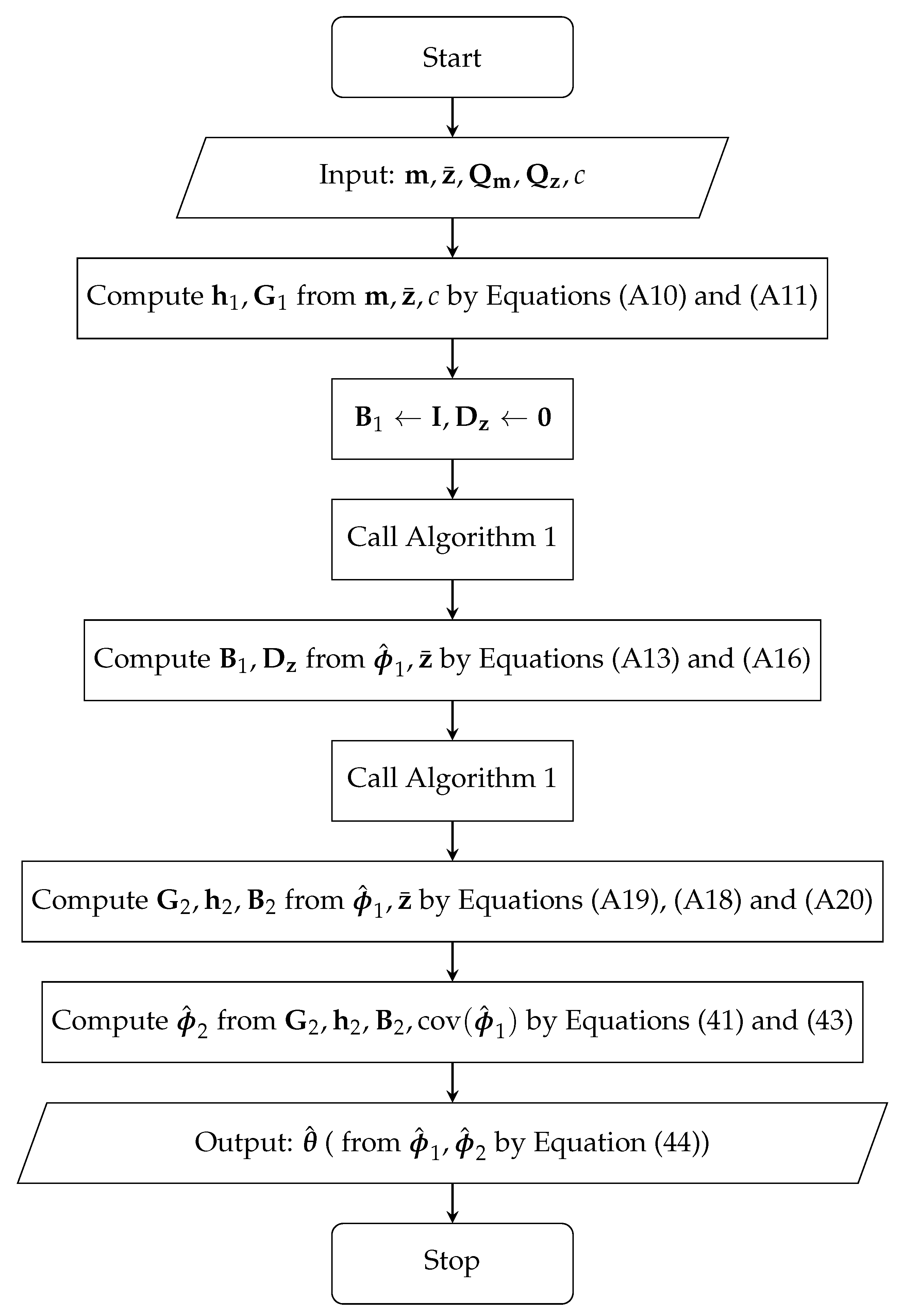
In order to set a benchmark before designing an estimator, we now evaluate the Hybrid Cramér–Rao Bound (HCRB) [36,37,38,39] for the hybrid parameter estimation problem proposed in Section 3. The HCRB provides a lower bound on the error covariance matrix of the estimator of a hybrid unknown parameter vector.

In our statistical model, the wanted parameter vector $\mathit{\theta }$ and the nuisance parameter vector (i.e., the actual sensor positions) $\mathbf{z}$ are both unknown. What makes them different is that $\mathit{\theta }$ is deterministic, and $\mathbf{z}$ is a random parameter vector. Such models arise in many applications where we want to investigate model uncertainty or environmental mismatch. Here, we consider $\mathit{\theta }$ and $\mathbf{z}$ together as a hybrid parameter vector

$$\gamma ={[{\mathit{\theta }}^{\mathrm{T}},{\mathbf{z}}^{\mathrm{T}}]}^{\mathrm{T}}.$$

(9)

Before moving on to the estimator design, we outline the procedures for deriving the HCRB. In such a hybrid parameter case, the HCRB is calculated using the joint probability density of the observed measurement vector $\mathbf{m}$ and the sensor position vector $\mathbf{z}$. The hybrid information matrix ${\mathbf{J}}_H$ can be expressed as the sum

$${\mathbf{J}}_H={\mathbf{J}}_D+{\mathbf{J}}_P,$$

(10)

where ${\mathbf{J}}_D$ represents the contribution of observations $\mathbf{m}$ and ${\mathbf{J}}_P$ represents the contribution of the prior knowledge on $\mathbf{z}$. Note that the unknown parameter vector $\gamma ={[{\mathit{\theta }}^{\mathrm{T}},{\mathbf{z}}^{\mathrm{T}}]}^{\mathrm{T}}$ is in the mean vector $\overline{\mathbf{m}}$ of the multivariate normal distribution in Equation (8) and $\mathbf{z}$ is a multivariate normal random vector itself as in Equation (3). Section 3 reveals that $\overline{\mathbf{m}}$ depends on $\mathit{\theta }$, $\mathbf{z}$ and c. In our model, the random parameter vector $\mathbf{z}$ does not depend on the deterministic parameter vector $\mathit{\theta }$. Thus, ${\mathbf{J}}_D$ and ${\mathbf{J}}_P$ is fairly easy to get [40]. Consequently,

$$\begin{array}{ccc}\hfill {\mathbf{J}}_D& =& E_{\mathbf{z}}\left\{{\left[\frac{\partial \overline{\mathbf{m}}}{\partial \gamma }\right]}^{\mathrm{T}}{\mathbf{Q}}_{\mathbf{m}}^{-1}\left[\frac{\partial \overline{\mathbf{m}}}{\partial \gamma }\right]\right\},\hfill \end{array}$$

(11)

$$\begin{array}{ccc}\hfill {\mathbf{J}}_P& =& blkdiag({\mathbf{0}}_{4\times 4},{\mathbf{Q}}_{\mathbf{z}}^{-1}).\hfill \end{array}$$

(12)

When the levels of sensor positions’ uncertainties are small, according to the approximation principle suggested by [41], the expected value matrix in Equation (11) can be approximated by replacing random vector $\mathbf{z}$ with its expected value vector $\overline{\mathbf{z}}$. Then, from the blockwise inversion of ${\mathbf{J}}_H{|}_{\mathbf{z}=\overline{\mathbf{z}}}$ and the matrix inversion lemma, we have the HCRB for the estimation of $\mathit{\theta }={[{\mathbf{u}}^{\mathrm{T}},{\dot{\mathbf{u}}}^{\mathrm{T}}]}^{\mathrm{T}}$ as follows:

$${HCRB}_{\mathit{\theta }}\approx {\left\{{\left(\frac{\partial \overline{\mathbf{m}}}{\partial \mathit{\theta }}\right)}^{\mathrm{T}}{\left[{\mathbf{Q}}_{\mathbf{m}}+\frac{\partial \overline{\mathbf{m}}}{\partial \mathbf{z}}{\mathbf{Q}}_{\mathbf{z}}{\left(\frac{\partial \overline{\mathbf{m}}}{\partial \mathbf{z}}\right)}^{\mathrm{T}}\right]}^{-1}\frac{\partial \overline{\mathbf{m}}}{\partial \mathit{\theta }}\right\}}^{-1}{|}_{\mathbf{z}=\overline{\mathbf{z}}}.$$

(13)

For numerical computation using Equation (13), $\frac{\partial \overline{\mathbf{m}}}{\partial \mathit{\theta }}$ and $\frac{\partial \overline{\mathbf{m}}}{\partial \mathbf{z}}$ are required. More information is available in Appendix A.

5. Estimator Design

In this section, we use Taylor expansion, introduce auxiliary variables and apply multi-stage processing to deal with the nonlinear estimation problem proposed in Section 3. In particular, our algorithm can be divided into two stages, each involving an unconstrained linear weighted least squares (WLS) computation which is computationally attractive. During the algorithm design and performance analysis of our estimator, it is necessary to use many matrix symbols to simplify the presentation. These matrices are shown in Table 2 for easy reference. When justifying the introduction of these matrices, we find that these matrices naturally arise in a general weighted least squares problem. To prevent ourselves from obscuring the design of the estimator, the reader is referred to the Appendix B.

Table 2. List of matrix symbols.

Matrix Notations	Expressions
${\mathbf{P}}_1$	${\mathbf{G}}_1^{\mathrm{T}}{\mathbf{W}}_1{\mathbf{G}}_1$
${\mathbf{P}}_2$	${\mathbf{G}}_2^{\mathrm{T}}{\mathbf{W}}_2{\mathbf{G}}_2$
${\mathbf{H}}_1$	${{\mathbf{P}}_1}^{-1}{{\mathbf{G}}_1}^{\mathrm{T}}{\mathbf{W}}_1$
${\mathbf{H}}_2$	${{\mathbf{P}}_2}^{-1}{{\mathbf{G}}_2}^{\mathrm{T}}{\mathbf{W}}_2$
${\mathbf{K}}_1$	${\mathbf{W}}_1(\mathbf{I}-{\mathbf{G}}_1^o{\mathbf{H}}_1^o)$
${\mathbf{K}}_2$	${\mathbf{W}}_2(\mathbf{I}-{\mathbf{G}}_2^o{\mathbf{H}}_2^o)$
$\mathbf{U}$	${\mathbf{W}}_2^{-1}{\mathbf{K}}_2$
$\mathbf{V}$	${\mathbf{H}}_2^o{\mathbf{W}}_2^{-1}$

Based on the Conditions 1 through 4 in Section 3, it follows from the first-order Taylor’s formula that

$$\begin{array}{ccc}\hfill \parallel \mathbf{u}-{\mathbf{t}}_i\parallel & \approx & \parallel \mathbf{u}-{\overline{\mathbf{t}}}_i\parallel +{\rho }_{{\overline{\mathbf{t}}}_i,\mathbf{u}}^{\mathrm{T}}\mathsf{\Delta }{\mathbf{t}}_i,\hfill \end{array}$$

(14)

$$\begin{array}{ccc}\hfill \parallel \mathbf{u}-{\mathbf{s}}_j\parallel & \approx & \parallel \mathbf{u}-{\overline{\mathbf{s}}}_j\parallel +{\rho }_{{\overline{\mathbf{s}}}_j,\mathbf{u}}^{\mathrm{T}}\mathsf{\Delta }{\mathbf{s}}_j,\hfill \end{array}$$

(15)

$$\begin{array}{ccc}\hfill \parallel {\mathbf{t}}_i-{\mathbf{s}}_j\parallel & \approx & \parallel {\overline{\mathbf{t}}}_i-{\overline{\mathbf{s}}}_j\parallel +{\rho }_{{\overline{\mathbf{t}}}_i,{\overline{\mathbf{s}}}_j}^{\mathrm{T}}(\mathsf{\Delta }{\mathbf{t}}_i-\mathsf{\Delta }{\mathbf{s}}_j),\hfill \end{array}$$

(16)

$$\begin{array}{ccc}\hfill {\rho }_{\mathbf{u},{\mathbf{t}}_i}& \approx & {\rho }_{\mathbf{u},{\overline{\mathbf{t}}}_i}-{\mathbf{A}}_{\mathbf{u},{\overline{\mathbf{t}}}_i}\mathsf{\Delta }{\mathbf{t}}_i,\hfill \end{array}$$

(17)

$$\begin{array}{ccc}\hfill {\rho }_{\mathbf{u},{\mathbf{s}}_j}& \approx & {\rho }_{\mathbf{u},{\overline{\mathbf{s}}}_j}-{\mathbf{A}}_{\mathbf{u},{\overline{\mathbf{s}}}_j}\mathsf{\Delta }{\mathbf{s}}_j.\hfill \end{array}$$

(18)

If we plug Equation (14) through Equation (16) into Equation (4), we obtain

$$c{\tau }_{i,j}\approx \parallel \mathbf{u}-{\overline{\mathbf{t}}}_i\parallel +\parallel \mathbf{u}-{\overline{\mathbf{s}}}_j\parallel -\parallel {\overline{\mathbf{t}}}_i-{\overline{\mathbf{s}}}_j\parallel +{ϵ}_{\tau ,i,j},$$

(19)

where

$${ϵ}_{\tau ,i,j}={\rho }_{{\overline{\mathbf{t}}}_i,\mathbf{u}}^{\mathrm{T}}\mathsf{\Delta }{\mathbf{t}}_i+{\rho }_{{\overline{\mathbf{s}}}_j,\mathbf{u}}^{\mathrm{T}}\mathsf{\Delta }{\mathbf{s}}_j-{\rho }_{{\overline{\mathbf{t}}}_i,{\overline{\mathbf{s}}}_j}^{\mathrm{T}}(\mathsf{\Delta }{\mathbf{t}}_i-\mathsf{\Delta }{\mathbf{s}}_j)+c\mathsf{\Delta }{\tau }_{i,j}.$$

(20)

Furthermore, inserting Equation (17) and Equation (18) into Equation (5) gives

$$c{f}_{i,j}\simeq {\rho }_{\mathbf{u},{\overline{\mathbf{t}}}_i}^{\mathrm{T}}\dot{\mathbf{u}}+{\rho }_{\mathbf{u},{\overline{\mathbf{s}}}_j}^{\mathrm{T}}\dot{\mathbf{u}}+{ϵ}_{f,i,j},$$

(21)

where

$${ϵ}_{f,i,j}=-{(A_{\mathbf{u},{\overline{\mathbf{t}}}_i}\dot{\mathbf{u}})}^{\mathrm{T}}\mathsf{\Delta }{\mathbf{t}}_i-{(A_{\mathbf{u},{\overline{\mathbf{s}}}_j}\dot{\mathbf{u}})}^{\mathrm{T}}\mathsf{\Delta }{\mathbf{s}}_j+c\mathsf{\Delta }{f}_{i,j}.$$

(22)

5.1. First Stage

Without loss of generality, let $M<N$. Move $(\parallel \mathbf{u}-{\overline{\mathbf{t}}}_i\parallel -\parallel {\overline{\mathbf{t}}}_i-{\overline{\mathbf{s}}}_j\parallel )$ from the right side to the left side in Equation (19), and square both sides. Then, we see that

$$\begin{array}{cc}\hfill & 2\parallel \mathbf{u}-{\overline{\mathbf{s}}}_j\parallel {ϵ}_{\tau ,i,j}+{ϵ}_{\tau ,i,j}^2\hfill \\ \hfill \approx & 2{\overline{\mathbf{t}}}_i^{\mathrm{T}}({\overline{\mathbf{t}}}_i-{\overline{\mathbf{s}}}_j)+2c{\tau }_{i,j}\parallel {\overline{\mathbf{t}}}_i-{\overline{\mathbf{s}}}_j\parallel +c^2{\tau }_{i,j}^2\hfill \\ \hfill & -2{({\overline{\mathbf{t}}}_i-{\overline{\mathbf{s}}}_j)}^{\mathrm{T}}\mathbf{u}-2(c{\tau }_{i,j}+\parallel {\overline{\mathbf{t}}}_i-{\overline{\mathbf{s}}}_j\parallel )\parallel \mathbf{u}-{\overline{\mathbf{t}}}_i\parallel .\hfill \end{array}$$

(23)

Applying similar procedures to Equation (21) gives

$$\begin{array}{cc}\hfill & \parallel \mathbf{u}-{\overline{\mathbf{s}}}_j\parallel {ϵ}_{f,i,j}+{\rho }_{\mathbf{u},\overline{{\mathbf{s}}_j}}^{\mathrm{T}}\dot{\mathbf{u}}{ϵ}_{\tau ,i,j}+{ϵ}_{\tau ,i,j}{ϵ}_{f,i,j}\hfill \\ \hfill \approx & c{f}_{i,j}\parallel {\overline{\mathbf{t}}}_i-{\overline{\mathbf{s}}}_j\parallel +c^2{\tau }_{i,j}{f}_{i,j}\hfill \\ \hfill & -c{f}_{i,j}\parallel \mathbf{u}-{\overline{\mathbf{t}}}_i\parallel -{({\overline{\mathbf{t}}}_i-{\overline{\mathbf{s}}}_j)}^{\mathrm{T}}\dot{\mathbf{u}}\hfill \\ \hfill & -(c{\tau }_{i,j}+\parallel {\overline{\mathbf{t}}}_i-{\overline{\mathbf{s}}}_j\parallel ){\rho }_{\mathbf{u},{\overline{\mathbf{t}}}_i}^{\mathrm{T}}\dot{\mathbf{u}}.\hfill \end{array}$$

(24)

If we define an unknown parameter vector as

$${\mathit{\varphi }}_1={[{\mathbf{u}}^{\mathrm{T}},{\mathit{\alpha }}^{\mathrm{T}},{\dot{\mathbf{u}}}^{\mathrm{T}},{\mathit{\beta }}^{\mathrm{T}}]}^{\mathrm{T}},$$

(25)

where

$$\begin{array}{ccc}\hfill \mathit{\alpha }& =& {[{\alpha }_1,{\alpha }_2,\dots ,{\alpha }_M]}^{\mathrm{T}},\hfill \end{array}$$

(26)

$$\begin{array}{ccc}\hfill \mathit{\beta }& =& {[{\beta }_1,{\beta }_2,\dots ,{\beta }_M]}^{\mathrm{T}},\hfill \end{array}$$

(27)

$$\begin{array}{ccc}\hfill {\alpha }_i& =& \parallel \mathbf{u}-{\overline{\mathbf{t}}}_i\parallel ,i=1,2,\dots ,M,\hfill \end{array}$$

(28)

$$\begin{array}{ccc}\hfill {\beta }_i& =& {\rho }_{\mathbf{u},{\overline{\mathbf{t}}}_i}^{\mathrm{T}}\dot{\mathbf{u}},i=1,2,\dots ,M,\hfill \end{array}$$

(29)

then a linear system of equations can be obtained from Equation (23) and Equation (24) as

$${\mathbf{B}}_1{\mathit{ϵ}}_1^{(1)}+{\mathit{ϵ}}_1^{(2)}\approx {\mathbf{h}}_1-{\mathbf{G}}_1{\mathit{\varphi }}_1.$$

(30)

We leave the details of ${\mathbf{h}}_1$, ${\mathbf{G}}_1$, ${\mathbf{B}}_1$, ${\mathit{ϵ}}_1^{(1)}$ and ${\mathit{ϵ}}_1^{(2)}$ presented in Appendix C. Note that ${\mathit{ϵ}}_1^{(1)}$ and ${\mathit{ϵ}}_1^{(2)}$ are first-order and second-order approximation error respectively.

By ignoring the second-order error term ${\mathit{ϵ}}_1^{(2)}$, the WLS solution to Equation (30) is

$${\widehat{\mathit{\varphi }}}_1={\mathbf{H}}_1{\mathbf{h}}_1,$$

(31)

and has covariance matrix

$$cov({\widehat{\mathit{\varphi }}}_1)=cov(\mathsf{\Delta }{\mathit{\varphi }}_1)\approx {{\mathbf{P}}_1^o}^{-1},$$

(32)

where ${\mathbf{H}}_1={{\mathbf{P}}_1}^{-1}{{\mathbf{G}}_1}^{\mathrm{T}}{\mathbf{W}}_1$, ${\mathbf{P}}_1={\mathbf{G}}_1^{\mathrm{T}}{\mathbf{W}}_1{\mathbf{G}}_1$ and ${\mathbf{P}}_1^o$ is the zero-order approximation of ${\mathbf{P}}_1$. The weighting matrix ${\mathbf{W}}_1$ is the inverse of the covariance matrix of the approximation error ${\mathbf{B}}_1{\mathit{ϵ}}_1^{(1)}$, that is,

$$\begin{array}{cc}\hfill {\mathbf{W}}_1=& {[E({\mathbf{B}}_1{\mathit{ϵ}}_1^{(1)}{{\mathit{ϵ}}_1^{(1)}}^{\mathrm{T}}{\mathbf{B}}_1^{\mathrm{T}})]}^{-1}\hfill \\ \hfill =& {\mathbf{B}}_1^{-\mathrm{T}}cov{({\mathit{ϵ}}_1^{(1)})}^{-1}{\mathbf{B}}_1^{-1}.\hfill \end{array}$$

(33)

The computation of $cov({\mathit{ϵ}}_1^{(1)})$ is straightforward. Because of the assumed statistical independence between $\mathsf{\Delta }\mathbf{z}$ and $\mathsf{\Delta }\mathbf{m}$ in Equation (A15),

$$cov({\mathit{ϵ}}_1^{(1)})={\mathbf{D}}_{\mathbf{z}}{\mathbf{Q}}_{\mathbf{z}}{\mathbf{D}}_{\mathbf{z}}^{\mathrm{T}}+c^2{\mathbf{Q}}_{\mathbf{m}},$$

(34)

where ${\mathbf{D}}_{\mathbf{z}}$ is shown in Equation (A16).

We get Equation (32) by the first-order perturbation analysis.

$$\begin{array}{cc}\hfill cov(\mathsf{\Delta }{\varphi }_1)& \approx E[{\mathbf{H}}_1^o{\mathbf{B}}_1{\mathit{ϵ}}_1^{(1)}·{({\mathbf{H}}_1^o{\mathbf{B}}_1{\mathit{ϵ}}_1^{(1)})}^{\mathrm{T}}]\hfill \\ \hfill & ={\mathbf{H}}_1^o·{\mathbf{B}}_{1}cov({\mathit{ϵ}}_1^{(1)}){\mathbf{B}}_1^{\mathrm{T}}·{{\mathbf{H}}_1^o}^{\mathrm{T}}\hfill \\ \hfill & ={{\mathbf{P}}_1^o}^{-1}{{\mathbf{G}}_1^o}^{\mathrm{T}}{\mathbf{W}}_1·{\mathbf{W}}_1^{-1}·{\mathbf{W}}_1^{\mathrm{T}}{\mathbf{G}}_1^o{{\mathbf{P}}_1^o}^{-\mathrm{T}}\hfill \\ \hfill & ={{\mathbf{P}}_1^o}^{-1}·{{\mathbf{G}}_1^o}^{\mathrm{T}}{\mathbf{W}}_1^{\mathrm{T}}{\mathbf{G}}_1^o·{{\mathbf{P}}_1^o}^{-\mathrm{T}}\hfill \\ \hfill & ={{\mathbf{P}}_1^o}^{-1}{{\mathbf{P}}_1^o}^{\mathrm{T}}{{\mathbf{P}}_1^o}^{-\mathrm{T}}\hfill \\ \hfill & ={{\mathbf{P}}_1^o}^{-1}.\hfill \end{array}$$

(35)

5.2. Second Stage

With ${\widehat{\mathit{\varphi }}}_1$ and its covariance matrix ${{\mathbf{P}}_1^o}^{-1}$, the aim of the second stage is to estimate the estimation error vector introduced in the first stage. In order to use symbols similar to the first stage, we denote this estimation error vector as ${\mathit{\varphi }}_2$, i.e.,

$${\mathit{\varphi }}_2={[\mathsf{\Delta }{\mathbf{u}}^{\mathrm{T}},\mathsf{\Delta }{\dot{\mathbf{u}}}^{\mathrm{T}}]}^{\mathrm{T}}=\mathsf{\Delta }{\mathit{\varphi }}_1([1,2,M+3,M+4]).$$

(36)

By substituting $\mathbf{u}=\widehat{\mathbf{u}}-\mathsf{\Delta }\mathbf{u}$ and ${\alpha }_i={\widehat{\alpha }}_i-\mathsf{\Delta }{\alpha }_i$ into ${\alpha }_i^2={\parallel \mathbf{u}-{\overline{\mathbf{t}}}_i\parallel }^2$, we obtain

$$\begin{array}{cc}\hfill & 2{\alpha }_i\mathsf{\Delta }{\alpha }_i+{\parallel \mathsf{\Delta }\mathbf{u}\parallel }^2+{(\mathsf{\Delta }{\alpha }_i)}^2\hfill \\ \hfill =& {\widehat{{\alpha }_i}}^2-{\parallel \widehat{\mathbf{u}}-{\overline{\mathbf{t}}}_i\parallel }^2+2{(\widehat{\mathbf{u}}-{\overline{\mathbf{t}}}_i)}^{\mathrm{T}}\mathsf{\Delta }\mathbf{u}.\hfill \end{array}$$

(37)

Furthermore, plugging ${\alpha }_i={\widehat{\alpha }}_i-\mathsf{\Delta }{\alpha }_i$, ${\beta }_i={\widehat{\beta }}_i-\mathsf{\Delta }{\beta }_i$, $\mathbf{u}=\widehat{\mathbf{u}}-\mathsf{\Delta }\mathbf{u}$ and $\dot{\mathbf{u}}=\widehat{\dot{\mathbf{u}}}-\mathsf{\Delta }\dot{\mathbf{u}}$ into ${\alpha }_i{\beta }_i={(\mathbf{u}-{\overline{\mathbf{t}}}_i)}^{\mathrm{T}}\dot{\mathbf{u}}$ gives

$$\begin{array}{cc}\hfill & {\beta }_i\mathsf{\Delta }{\alpha }_i+{\alpha }_i\mathsf{\Delta }{\beta }_i+\mathsf{\Delta }{\alpha }_i\mathsf{\Delta }{\beta }_i+\mathsf{\Delta }{\mathbf{u}}^{\mathrm{T}}\mathsf{\Delta }\dot{\mathbf{u}}\hfill \\ \hfill =& {\widehat{\alpha }}_i{\widehat{\beta }}_i-{(\widehat{\mathbf{u}}-{\overline{\mathbf{t}}}_i)}^{\mathrm{T}}\widehat{\dot{\mathbf{u}}}+{\widehat{\dot{\mathbf{u}}}}^{\mathrm{T}}\mathsf{\Delta }\mathbf{u}+{(\widehat{\mathbf{u}}-{\overline{\mathbf{t}}}_i)}^{\mathrm{T}}\mathsf{\Delta }\dot{\mathbf{u}}.\hfill \end{array}$$

(38)

In matrix notation, from Equation (37) and Equation (38), we have

$${\mathbf{B}}_2{\mathit{ϵ}}_2^{(1)}+{\mathit{ϵ}}_2^{(2)}={\mathbf{h}}_2-{\mathbf{G}}_2{\mathit{\varphi }}_2,$$

(39)

where

$${\mathit{ϵ}}_2^{(1)}=\mathsf{\Delta }{\mathit{\varphi }}_1,$$

(40)

i.e., the estimation error in the first stage $\mathsf{\Delta }{\mathit{\varphi }}_1$ is considered as the first-order approximation error in the second stage. This is a key point of our estimator. The details of ${\mathbf{h}}_2$, ${\mathbf{G}}_2$, ${\mathbf{B}}_2$ and the second-order approximation error ${\mathit{ϵ}}_2^{(2)}$ can be found in Appendix D.

By ignoring the second-order error term ${\mathit{ϵ}}_2^{(2)}$ and following the first stage’s approach, the WLS solution to Equation (39) is

$${\widehat{\mathit{\varphi }}}_2={\mathbf{H}}_2{\mathbf{h}}_2,$$

(41)

and has error covariance matrix

$$cov(\mathsf{\Delta }{\mathit{\varphi }}_2)\approx {{\mathbf{P}}_2^o}^{-1},$$

(42)

where ${\mathbf{H}}_2={{\mathbf{P}}_2}^{-1}{{\mathbf{G}}_2}^{\mathrm{T}}{\mathbf{W}}_2$, ${\mathbf{P}}_2={\mathbf{G}}_2^{\mathrm{T}}{\mathbf{W}}_2{\mathbf{G}}_2$ and ${\mathbf{P}}_2^o$ is the zero-order approximation of ${\mathbf{P}}_2$. The weighting matrix ${\mathbf{W}}_2$ is the inverse of the covariance matrix of the approximation error ${\mathbf{B}}_2{\mathit{ϵ}}_2^{(1)}$, that is,

$$\begin{array}{cc}\hfill {\mathbf{W}}_2\approx & E{({\mathbf{B}}_2{\mathit{ϵ}}_2^{(1)}{{\mathit{ϵ}}_2^{(1)}}^{\mathrm{T}}{{\mathbf{B}}_2}^{\mathrm{T}})}^{-1}\hfill \\ \hfill \approx & {{\mathbf{B}}_2}^{-\mathrm{T}}{\mathbf{P}}_1^o{{\mathbf{B}}_2}^{-1}.\hfill \end{array}$$

(43)

Finally, our estimator can be constructed from ${\widehat{\mathit{\varphi }}}_1$ in Equation (31) and ${\widehat{\mathit{\varphi }}}_2$ in Equation (41) as

$$\widehat{\mathit{\theta }}={[{\widehat{\mathit{\varphi }}}_1{(1:2)}^{\mathrm{T}},{\widehat{\mathit{\varphi }}}_1{(M+3:M+4)}^{\mathrm{T}}]}^{\mathrm{T}}-{\widehat{\mathit{\varphi }}}_2.$$

(44)

Last but not least, some obstacles arise in the practical computation of our estimator. In the first stage, ${\mathbf{B}}_1$ and ${\mathbf{D}}_{\mathbf{z}}$, as shown in Equation (A13) and Equation (A16), involve $\mathbf{u}$ and $\dot{\mathbf{u}}$ which are unavailable for the algorithm. To resolve this problem, we first assign an identity matrix to ${\mathbf{B}}_1$ and an all-zero matrix to ${\mathbf{D}}_{\mathbf{z}}$ to get coarse estimates of $\mathbf{u}$ and $\dot{\mathbf{u}}$ from Equation (31), and then substitute the coarse estimates into Equation (A13) and Equation (A16) to update ${\mathbf{B}}_1$ and ${\mathbf{D}}_{\mathbf{z}}$. Confronted with similar problems in the second stage in Equation (A20), we substitute $\widehat{\mathit{\alpha }}$ and $\widehat{\mathit{\beta }}$ for computing ${\mathbf{B}}_2$, resulting ${\widehat{\mathbf{B}}}_2$ and ${\widehat{\mathbf{W}}}_2$. These approximations will be considered properly in the statistical performance analysis in Section 6.

5.3. Summary

As a guide to implementation, the flowchart of the proposed estimator is shown in Figure 1 and the algorithm of the first stage of our estimator is summarized in Algorithm 1.

Algorithm 1 First stage of the estimator.

1: procedureEstimator-First-Stage(${\mathbf{Q}}_{\mathbf{m}},{\mathbf{Q}}_{\mathbf{z}},c,{\mathbf{G}}_1,{\mathbf{h}}_1,{\mathbf{D}}_{\mathbf{z}},{\mathbf{B}}_1$) 2:     Compute $cov({\mathit{ϵ}}_1^{(1)})$ from ${\mathbf{Q}}_{\mathbf{m}},{\mathbf{Q}}_{\mathbf{z}},{\mathbf{D}}_{\mathbf{z}},c$ by Equation (34) 3:     Compute ${\mathbf{W}}_1$ from $cov({\mathit{ϵ}}_{\mathbf{1}}),{\mathbf{B}}_1$ by Equation (33) 4:     return ${\widehat{\mathit{\varphi }}}_1$ from ${\mathbf{G}}_1,{\mathbf{h}}_1,{\mathbf{W}}_1$ by Equation (31) 5:     return $cov({\widehat{\mathit{\varphi }}}_1)$ from ${\mathbf{G}}_1,{\mathbf{W}}_1$ by Equation (32) 6: end procedure

Figure 1. Flowchart of the proposed estimator. Algorithm 1 is called in the flowchart.

6. Performance Analysis

The covariance matrix and the bias vector are the two most important numerical characterization of a vector estimator. The perturbations in the design matrices (i.e., ${\mathbf{G}}_1$ and ${\mathbf{G}}_2$) and the higher-order noise terms in the observation vector (i.e., ${\mathbf{h}}_1$ and ${\mathbf{h}}_2$) in Equation (30) and Equation (39) make the conditions of Gauss–Markov theorem no longer true.

6.1. Bias Vector

We first derive the covariance matrix of our estimator in Equation (44). The bias analysis here will be up to the second-order statistics of the observation errors and the sensor position errors, i.e., the random terms higher than the second-order are ignored. Matrix differential calculus presented in [42] is intensively used in this subsection.

It can be seen from Equation (44) that the total bias vector of our estimator $\widehat{\mathit{\theta }}$ is

$${[{\mathit{\mu }}_1{(1:2)}^{\mathrm{T}},{\mathit{\mu }}_1{(M+3:M+4)}^{\mathrm{T}}]}^{\mathrm{T}}-{\mathit{\mu }}_2,$$

(45)

where ${\mathit{\mu }}_1$ and ${\mathit{\mu }}_2$ are the bias vectors of ${\widehat{\mathit{\varphi }}}_1$ and ${\widehat{\mathit{\varphi }}}_2$, respectively. The rest of our task is to compute the bias vector in the first stage and second stage, i.e., ${\mathit{\mu }}_1$ and ${\mathit{\mu }}_2$. We reiterate that the random terms higher than the second-order will be ignored at each occurrence of the approximately equal symbol. Please reference Table 2 for the matrix symbols involved.

The error of ${\widehat{\mathit{\varphi }}}_1$ is

$$\begin{array}{cc}\hfill \mathsf{\Delta }{\mathit{\varphi }}_1& ={\widehat{\mathit{\varphi }}}_1-{\mathit{\varphi }}_1\hfill \\ \hfill & \approx {\mathbf{H}}_1({\mathbf{B}}_1{\mathit{ϵ}}_1^{(1)}+{\mathit{ϵ}}_1^{(2)})\hfill \\ \hfill & \approx {\mathbf{H}}_1^o({\mathbf{B}}_1{\mathit{ϵ}}_1^{(1)}+{\mathit{ϵ}}_1^{(2)})+\mathsf{\Delta }{\mathbf{H}}_1·{\mathbf{B}}_1{ϵ}_1^{(1)},\hfill \end{array}$$

(46)

where $\mathsf{\Delta }{\mathbf{H}}_1$ and its related differentials can be obtained by matrix differential as follows:

$$\begin{array}{ccc}\hfill \mathsf{\Delta }{\mathbf{H}}_1& =& {{\mathbf{P}}_1^o}^{-1}\mathsf{\Delta }{\mathbf{G}}_1^{\mathrm{T}}{\mathbf{W}}_1+\mathsf{\Delta }({\mathbf{P}}_1^{-1}){{\mathbf{G}}_1^o}^{\mathrm{T}}{\mathbf{W}}_1,\hfill \end{array}$$

(47)

$$\begin{array}{ccc}\hfill \mathsf{\Delta }({\mathbf{P}}_1^{-1})& =& -{{\mathbf{P}}_1^o}^{-1}\mathsf{\Delta }{\mathbf{P}}_1{{\mathbf{P}}_1^o}^{-1},\hfill \end{array}$$

(48)

$$\begin{array}{ccc}\hfill \mathsf{\Delta }{\mathbf{P}}_1& =& {\mathsf{\Delta }{\mathbf{G}}_1}^{\mathrm{T}}{\mathbf{W}}_1{\mathbf{G}}_1^o+{{\mathbf{G}}_1^o}^{\mathrm{T}}{\mathbf{W}}_1\mathsf{\Delta }{\mathbf{G}}_1.\hfill \end{array}$$

(49)

Putting Equation (47) through Equation (49) into Equation (46) gives the estimation error vector in the first stage

$$\mathsf{\Delta }{\mathit{\varphi }}_1\approx \left({\mathbf{H}}_1^o·{\mathbf{B}}_1{\mathit{ϵ}}_1^{(1)}+{\mathbf{H}}_1^o{\mathit{ϵ}}_1^{(2)}\right)+\left({{\mathbf{P}}_1^o}^{-1}\mathsf{\Delta }{\mathbf{G}}_1^{\mathrm{T}}{\mathbf{K}}_1·{\mathbf{B}}_1{\mathit{ϵ}}_1^{(1)}-{\mathbf{H}}_1^o\mathsf{\Delta }{\mathbf{G}}_1{\mathbf{H}}_1^o·{\mathbf{B}}_1{\mathit{ϵ}}_1^{(1)}\right).$$

(50)

We note that the weight matrix ${\mathbf{W}}_1$ has no random errors in the first stage.

As in the first stage, the estimation error vector in the second stage is

$$\begin{array}{cc}\hfill \mathsf{\Delta }{\mathit{\varphi }}_2& ={\widehat{\mathit{\varphi }}}_2-{\mathit{\varphi }}_2\hfill \\ \hfill & ={\mathbf{H}}_2({\mathbf{B}}_2{\mathit{ϵ}}_2^{(1)}+{\mathit{ϵ}}_2^{(2)})\hfill \\ \hfill & \approx {\mathbf{H}}_2^o({\mathbf{B}}_2{\mathit{ϵ}}_2^{(1)}+{\mathit{ϵ}}_2^{(2)})+\mathsf{\Delta }{\mathbf{H}}_2·{\mathbf{B}}_2{\mathit{ϵ}}_2^{(1)}.\hfill \end{array}$$

(51)

Before moving on to the expression of $\mathsf{\Delta }{\mathbf{H}}_2$, we note that we use ${\widehat{\mathbf{B}}}_2$ rather than ${\mathbf{B}}_2$ in the practical implementation. So, $\mathsf{\Delta }{\mathbf{H}}_2$ can be obtained by matrix differential as follows:

$$\begin{array}{ccc}\hfill \mathsf{\Delta }{\mathbf{H}}_2& =& \mathsf{\Delta }({\mathbf{P}}_2^{-1}){{\mathbf{G}}_2^o}^{\mathrm{T}}{\mathbf{W}}_2+{{\mathbf{P}}_2^o}^{-1}\mathsf{\Delta }{\mathbf{G}}_2^{\mathrm{T}}{\mathbf{W}}_2+{{\mathbf{P}}_2^o}^{-1}{{\mathbf{G}}_2^o}^{\mathrm{T}}\mathsf{\Delta }{\mathbf{W}}_2,\hfill \end{array}$$

(52)

$$\begin{array}{ccc}\hfill \mathsf{\Delta }({\mathbf{P}}_2^{-1})& =& -{{\mathbf{P}}_2^o}^{-1}\mathsf{\Delta }{\mathbf{P}}_2{{\mathbf{P}}_2^o}^{-1},\hfill \end{array}$$

(53)

$$\begin{array}{ccc}\hfill \mathsf{\Delta }{\mathbf{P}}_2& =& \mathsf{\Delta }{\mathbf{G}}_2^{\mathrm{T}}{\mathbf{W}}_2{\mathbf{G}}_2^o+{{\mathbf{G}}_2^o}^{\mathrm{T}}{\mathbf{W}}_2\mathsf{\Delta }{\mathbf{G}}_2+{{\mathbf{G}}_2^o}^{\mathrm{T}}\mathsf{\Delta }{\mathbf{W}}_2{\mathbf{G}}_2^o,\hfill \end{array}$$

(54)

$$\begin{array}{ccc}\hfill \mathsf{\Delta }{\mathbf{W}}_2& =& {{\mathbf{B}}_2}^{-\mathrm{T}}\mathsf{\Delta }{\mathbf{P}}_1{{\mathbf{B}}_2}^{-1}-{\mathbf{W}}_2\mathsf{\Delta }{\mathbf{B}}_2{{\mathbf{B}}_2}^{-1}-{{\mathbf{B}}_2}^{-\mathrm{T}}\mathsf{\Delta }{\mathbf{B}}_2^{\mathrm{T}}{\mathbf{W}}_2.\hfill \end{array}$$

(55)

By comparing Equation (52) through Equation (54) with Equation (47) through Equation (49), we see that $\mathsf{\Delta }{\mathbf{W}}_2$ in Equation (55) contributes new perturbation resulted from practical implementation, which are introduced by $\mathsf{\Delta }{\mathbf{P}}_1$ and $\mathsf{\Delta }{\mathbf{B}}_2$. Furthermore, $\mathsf{\Delta }{\mathbf{P}}_1$ can be expressed with $\mathsf{\Delta }{\mathbf{G}}_1$ by Equation (49).

Then from Equation (51), combining Equation (52) through Equation (55) together with Equation (49) we have

$$\begin{array}{cc}\mathsf{\Delta }{\mathit{\varphi }}_2\approx & \left({\mathbf{H}}_2^o·{\mathbf{B}}_2{\mathit{ϵ}}_2^{(1)}+{\mathbf{H}}_2^o{\mathit{ϵ}}_2^{(2)}\right)+\left({{\mathbf{P}}_2^o}^{-1}\mathsf{\Delta }{\mathbf{G}}_2^{\mathrm{T}}{\mathbf{K}}_2·{\mathbf{B}}_2{\mathit{ϵ}}_2^{(1)}-{\mathbf{H}}_2^o\mathsf{\Delta }{\mathbf{G}}_2{\mathbf{H}}_2^o·{\mathbf{B}}_2{\mathit{ϵ}}_2^{(1)}\right)\hfill \\ & +\left(-{\mathbf{H}}_2^o\mathsf{\Delta }{\mathbf{B}}_2{\mathbf{B}}_2^{-1}\mathbf{U}·{\mathbf{B}}_2{\mathit{ϵ}}_2^{(1)}-\mathbf{V}·{{\mathbf{B}}_2}^{-}\mathrm{T}\mathsf{\Delta }{\mathbf{B}}_2^{\mathrm{T}}{\mathbf{K}}_2·{\mathbf{B}}_2{\mathit{ϵ}}_2^{(1)}\right)\hfill \\ & +\left(\mathbf{V}·{{\mathbf{B}}_2}^{-}\mathrm{T}·{{\mathbf{G}}_1^o}^{\mathrm{T}}{\mathbf{W}}_1\mathsf{\Delta }{\mathbf{G}}_1·{\mathbf{B}}_2^{-1}\mathbf{U}·{\mathbf{B}}_2{\mathbf{H}}_1^o{\mathbf{B}}_1{\mathit{ϵ}}_1^{(1)}+\mathbf{V}·{{\mathbf{B}}_2}^{-}\mathrm{T}·\mathsf{\Delta }{\mathbf{G}}_1^{\mathrm{T}}{\mathbf{W}}_1{\mathbf{G}}_1^o·{\mathbf{B}}_2^{-1}\mathbf{U}·{\mathbf{B}}_2{\mathbf{H}}_1^o{\mathbf{B}}_1{\mathit{ϵ}}_1^{(1)}\right).\hfill \end{array}$$

(56)

The last line above is by Equation (46) and Equation (49).

Finally, taking expectation of $\mathsf{\Delta }{\mathit{\varphi }}_1$ and $\mathsf{\Delta }{\mathit{\varphi }}_2$ will yield ${\mathit{\mu }}_1$ and ${\mathit{\mu }}_2$. This involves complicated matrix partitioning and multivariate statistical analysis. Interested readers may refer to Appendix E.

6.2. Covariance Matrix

We then derive the covariance matrix of our estimator. The covariance analysis here will be up to the first-order statistics of the estimator errors, i.e., the error terms higher than the first-order are ignored.

$$\begin{array}{cc}\hfill cov(\widehat{\mathit{\theta }})& =cov({\widehat{\mathit{\varphi }}}_1(1,2,M+3,M+4)-{\widehat{\mathit{\varphi }}}_2)\hfill \\ \hfill & =cov({\mathit{\varphi }}_1(1,2,M+3,M+4)+\mathsf{\Delta }{\mathit{\varphi }}_1(1,2,M+3,M+4)-{\mathit{\varphi }}_2-\mathsf{\Delta }{\mathit{\varphi }}_2)\hfill \\ \hfill & =cov({\mathit{\varphi }}_1(1,2,M+3,M+4)-\mathsf{\Delta }{\mathit{\varphi }}_2)(\mathrm{by}(36))\hfill \\ \hfill & =cov(\mathsf{\Delta }{\mathit{\varphi }}_2)\hfill \\ \hfill & \approx {{\mathbf{P}}_2^o}^{-1}.\hfill \end{array}$$

(57)

We note that Yang et al. have explicitly given the covariance matrix of the two-stage weighted least squares (TS-WLS) method as follows:

$$cov({\widehat{\mathit{\theta }}}_{\mathrm{TS}-\mathrm{WLS}})\approx {({{\mathbf{G}}_2^o}^{\mathrm{T}}{\mathbf{B}}_2^{-\mathrm{T}}{\mathbf{V}}_1^{-1}{\mathbf{B}}_2^{-1}{\mathbf{G}}_2^o)}^{-1},$$

(58)

where

$$\begin{array}{ccc}\hfill {\mathbf{V}}_1& =& {({{\mathbf{G}}_1^o}^{\mathrm{T}}{\tilde{\mathbf{W}}}_1{\mathbf{G}}_1^o)}^{-1}{{\mathbf{G}}_1^o}^{\mathrm{T}}{\tilde{\mathbf{W}}}_1{\mathbf{B}}_{1}cov({\mathit{ϵ}}_1^{(1)}){\mathbf{B}}_1^{\mathrm{T}}{\tilde{\mathbf{W}}}_1^{\mathrm{T}}{\mathbf{G}}_1^o{({{\mathbf{G}}_1^o}^{\mathrm{T}}{\tilde{\mathbf{W}}}_1{\mathbf{G}}_1^o)}^{-\mathrm{T}},\hfill \end{array}$$

(59)

$$\begin{array}{ccc}\hfill {\tilde{\mathbf{W}}}_1& =& {\mathbf{B}}_1^{-\mathrm{T}}{(c^2{\mathbf{Q}}_{\mathbf{m}})}^{-1}{\mathbf{B}}_1^{-1}.\hfill \end{array}$$

(60)

We now claim the following proposition.

Proposition 1.

$$cov({\widehat{\mathit{\theta }}}_{\mathrm{TS}-\mathrm{WLS}})⪰cov(\widehat{\mathit{\theta }}).$$

(61)

Proof. 

By Equation (57) and Equation (58), it is enough to prove

$${\mathbf{P}}_2^o⪰{{\mathbf{G}}_2^o}^{\mathrm{T}}{\mathbf{B}}_2^{-\mathrm{T}}{\mathbf{V}}_1^{-1}{\mathbf{B}}_2^{-1}{\mathbf{G}}_2^o.$$

(62)

To get started, we expand the left side of Equation (62).

$$\begin{array}{cc}\hfill {\mathbf{P}}_2^o& ={{\mathbf{G}}_2^o}^{\mathrm{T}}{\mathbf{W}}_2{\mathbf{G}}_2^o\hfill \\ \hfill & \approx {{\mathbf{G}}_2^o}^{\mathrm{T}}({{\mathbf{B}}_2}^{-\mathrm{T}}{\mathbf{P}}_1^o{{\mathbf{B}}_2}^{-1}){\mathbf{G}}_2^o(\mathrm{by}\mathrm{Equation}(43))\hfill \\ \hfill & ={{\mathbf{G}}_2^o}^{\mathrm{T}}{[{\mathbf{B}}_2{({{\mathbf{G}}_1^o}^{\mathrm{T}}{\mathbf{W}}_1{\mathbf{G}}_1^o)}^{-1}{\mathbf{B}}_2^{\mathrm{T}}]}^{-1}{\mathbf{G}}_2^o\hfill \\ \hfill & ={{\mathbf{G}}_2^o}^{\mathrm{T}}{\mathbf{B}}_2^{-\mathrm{T}}{{\mathbf{G}}_1^o}^{\mathrm{T}}{\mathbf{W}}_1{\mathbf{G}}_1^o{\mathbf{B}}_2^{-1}{\mathbf{G}}_2^o\hfill \\ \hfill & ={{\mathbf{G}}_2^o}^{\mathrm{T}}{\mathbf{B}}_2^{-\mathrm{T}}{\mathbf{V}}_2^{-1}{\mathbf{B}}_2^{-1}{\mathbf{G}}_2^o(\mathrm{by}\mathrm{Equation}(33)),\hfill \end{array}$$

(63)

where

$${\mathbf{V}}_2={[{{\mathbf{G}}_1^o}^{\mathrm{T}}{\mathbf{B}}_1^{-\mathrm{T}}cov{({\mathit{ϵ}}_1^{(1)})}^{-1}{\mathbf{B}}_1^{-1}{\mathbf{G}}_1^o]}^{-1}.$$

(64)

As ${\mathbf{B}}_2^{-1}{\mathbf{G}}_2^o$ has full column rank, to complete the proof, we need only show that

$${\mathbf{V}}_1⪰{\mathbf{V}}_2.$$

(65)

We can prove Equation (65) by Matrix Schwarz inequality (Lemma 1.1 in [43]). Because ${\mathbf{B}}_{1}cov({\mathit{ϵ}}_1^{(1)}){\mathbf{B}}_1^{\mathrm{T}}$ is positive-definite, we can provide a Cholesky factorization as follows:

$${\mathbf{B}}_{1}cov({\mathit{ϵ}}_1^{(1)}){\mathbf{B}}_1^{\mathrm{T}}={\mathbf{LL}}^{\mathrm{T}},$$

(66)

where $\mathbf{L}$ is a unique lower triangular matrix. Let

$$\mathbf{P}={\mathbf{L}}^{-1}{\mathbf{G}}_1^o,\mathbf{Q}={\mathbf{L}}^{\mathrm{T}}{\tilde{\mathbf{W}}}_1^{\mathrm{T}}{\mathbf{G}}_1^o{({{\mathbf{G}}_1^o}^{\mathrm{T}}{\tilde{\mathbf{W}}}_1{\mathbf{G}}_1^o)}^{-\mathrm{T}}.$$

(67)

By Matrix Schwarz inequality, we get

$${\mathbf{Q}}^{\mathrm{T}}\mathbf{Q}⪰{({\mathbf{P}}^{\mathrm{T}}\mathbf{Q})}^{\mathrm{T}}{({\mathbf{P}}^{\mathrm{T}}\mathbf{P})}^{-1}({\mathbf{P}}^{\mathrm{T}}\mathbf{Q}).$$

(68)

Then with a straightforward verification, we have

$${\mathbf{Q}}^{\mathrm{T}}\mathbf{Q}={\mathbf{V}}_1,{\mathbf{P}}^{\mathrm{T}}\mathbf{P}={\mathbf{V}}_2^{-1},{\mathbf{P}}^{\mathrm{T}}\mathbf{Q}=\mathbf{I}.$$

(69)

The equations above imply that ${\mathbf{V}}_1⪰{\mathbf{V}}_2$, as desired. □

We close this section by establishing the approximate statistical efficiency of our estimator as the proposition below shows.

Proposition 2.

When the small error conditions in 1 through 6 are satisfied,

$${HCRB}_{\theta }\approx cov(\widehat{\mathit{\theta }}).$$

(70)

Proof. 

In view of Equation (13) and Equation (57), we will prove that

$$\left\{{\left(\frac{\partial \overline{\mathbf{m}}}{\partial \mathit{\theta }}\right)}^{\mathrm{T}}{\left[{\mathbf{Q}}_{\mathbf{m}}+\frac{\partial \overline{\mathbf{m}}}{\partial \mathbf{z}}{\mathbf{Q}}_{\mathbf{z}}{\left(\frac{\partial \overline{\mathbf{m}}}{\partial \mathbf{z}}\right)}^{\mathrm{T}}\right]}^{-1}\frac{\partial \overline{\mathbf{m}}}{\partial \mathit{\theta }}\right\}{|}_{\mathbf{z}=\overline{\mathbf{z}}}\approx {\mathbf{P}}_2^o.$$

(71)

By Equations (63), (64) and (34), the right side of Equation (71) is

$${\mathbf{P}}_2^o={\mathbf{G}}_3^{\mathrm{T}}{({\mathbf{D}}_{\mathbf{z}}{\mathbf{Q}}_{\mathbf{z}}{\mathbf{D}}_{\mathbf{z}}^{\mathrm{T}}+c^2{\mathbf{Q}}_{\mathbf{m}})}^{-1}{\mathbf{G}}_3,$$

(72)

where

$${\mathbf{G}}_3={\mathbf{B}}_1^{-1}{\mathbf{G}}_1^o{\mathbf{B}}_2^{-1}{\mathbf{G}}_2^o.$$

(73)

Expanding Equation (73) (in Appendix F) and comparing it with Equation (A1), we can show that, under the small error conditions,

$${\mathbf{G}}_3\approx -c\frac{\partial \overline{\mathbf{m}}}{\partial \mathit{\theta }}{|}_{\mathbf{z}=\overline{\mathbf{z}}}.$$

(74)

Furthermore, comparing Equation (A16) with Equation (A2), we arrive at

$${\mathbf{D}}_{\mathbf{z}}\approx c\frac{\partial \overline{\mathbf{m}}}{\partial \mathbf{z}}{|}_{\mathbf{z}=\overline{\mathbf{z}}}.$$

(75)

If we plug Equation (74) and Equation (75) into Equation (72), we get Equation (71). □

6.3. Time and Space Complexity

The computational load of our algorithm is focused on solving WLS problems. Singular value decomposition (SVD) is an efficient algorithm for solving WLS problems. With the method of truncated SVD, the time complexity is $\mathcal{O}(2m{n}^2+n^3+mn+n)$ and the space complexity is $\mathcal{O}(3n^2+2mn+3n)$ for a matrix of size $m\times n$ [44].

To facilitate complexity analysis, we list the matrices involved in the algorithm and their sizes in Table 3. As can be seen from the table, under the assumptions that $M\ll N$, the computational complexity of the first stage is dominant in the total computational complexity. For the design matrix ${\mathbf{G}}_1$ in the first stage, $m=2MN$ and $n=2M+4$. By keeping the highest order term of N and its coefficient, it can be seen that our algorithm takes $\mathcal{O}(N[4(4M^3+17M^2+18M)])$ time and $\mathcal{O}(N[8M(M+2)])$ space. In summary, our algorithm has linear complexity both in time and space.

Table 3. Size of matrices.

Matrix Notations	Matrix Sizes
${\mathbf{G}}_1$	$(2MN)\times (2M+4)$
${\mathit{\varphi }}_1$	$(2M+4)\times 1$
${\mathbf{h}}_1$	$(2MN)\times 1$
${\mathbf{B}}_1$	$(2MN)\times (2MN)$
${\mathbf{W}}_1$	$(2MN)\times (2MN)$
${\mathbf{G}}_{1,i}$	$(2N)\times (2M+4)$
${\mathbf{B}}_{1,i}$	$(2N)\times (2N)$
${\mathbf{G}}_2$	$(2M+4)\times 4$
${\mathit{\varphi }}_2$	$4\times 1$
${\mathbf{h}}_2$	$(2M+4)\times 1$
${\mathbf{B}}_2$	$(2M+4)\times (2M+4)$
${\mathbf{W}}_2$	$(2M+4)\times (2M+4)$
${\mathbf{Q}}_{\mathbf{m}}$	$(2MN)\times (2MN)$
${\mathbf{Q}}_{\mathbf{z}}$	$(2M+2N)\times (2M+2N)$
${\mathbf{D}}_{\mathbf{z}}$	$(2MN)\times (2M+2N)$

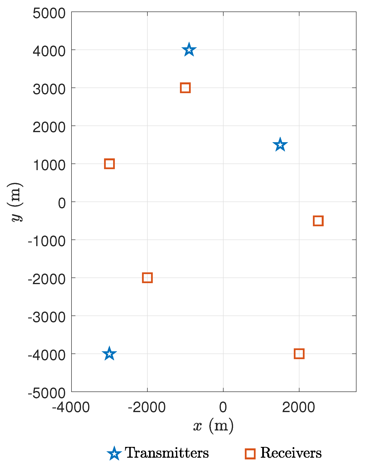
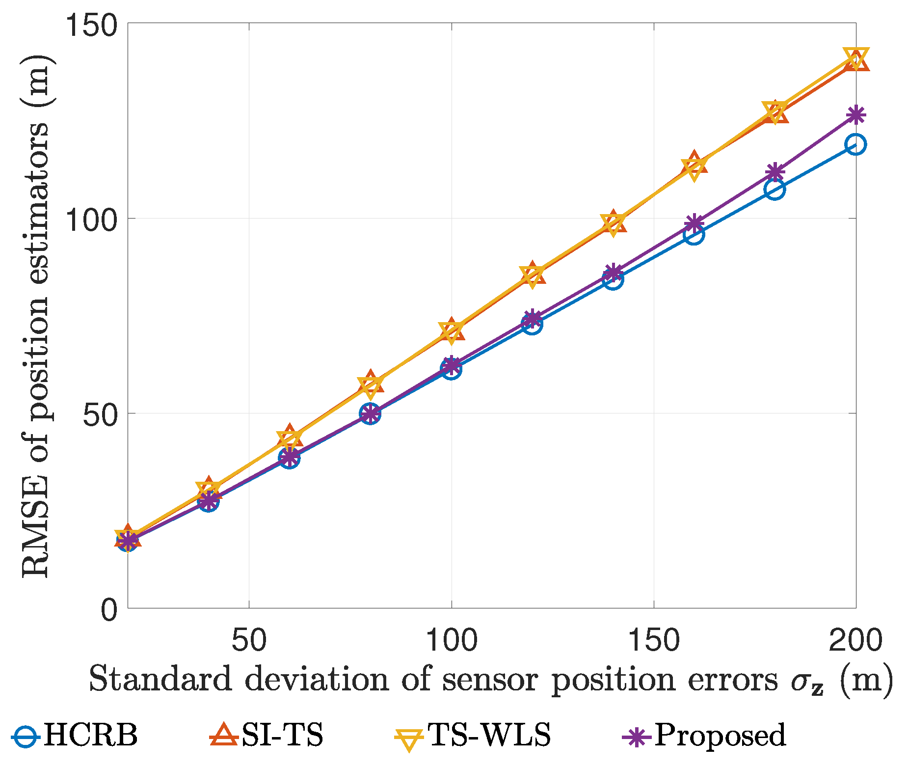
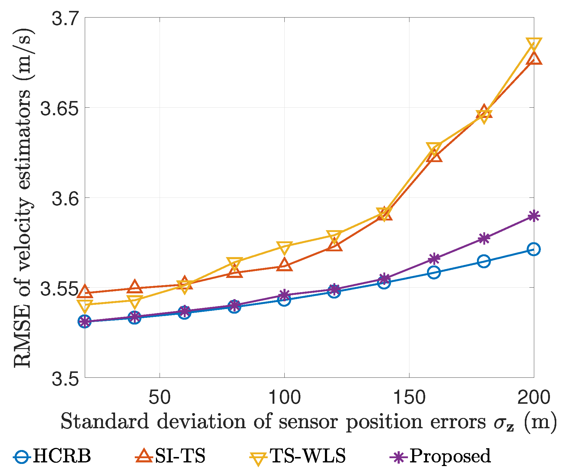
7. Results and Discussion

In the previous section, we have theoretically analyzed the performance of our estimator. Now we ascertain the performance of our estimator via computer simulations. Our simulations are divided into four subsections. Section 7.1 compares the error covariance matrix of our estimator with HCRB and the ones of two typical estimators, i.e., the spherical-interpolation initialized Taylor series method (SI-TS) [28,45] and TS-WLS [5]. Then, surface plots of the biases are shown in Section 7.2. In Section 7.3, we empirically explore the time complexity of our estimator for locating multiple disjoint targets. Finally, we use 80 randomly generated large-scale localization scenarios to further test the proposed estimator in Section 7.4.

The first three subsections base on the simulation settings of [6]. Specifically, the simulations use $M=3$ transmitters and $N=5$ receivers to determine the unknown position $\mathbf{u}$ and velocity $\dot{\mathbf{u}}$ of a moving target. As in [6], the nominal positions of the sensors are known and given as follows. ${\overline{\mathbf{t}}}_1={[1500,1500]}^{\mathrm{T}}$ m, ${\overline{\mathbf{t}}}_2={[-900,4000]}^{\mathrm{T}}$ m, ${\overline{\mathbf{t}}}_3={[-3000,-4000]}^{\mathrm{T}}$ m, ${\overline{\mathbf{s}}}_1={[-1000,3000]}^{\mathrm{T}}$ m, ${\overline{\mathbf{s}}}_2={[2500,-500]}^{\mathrm{T}}$ m, ${\overline{\mathbf{s}}}_3={[-3000,1000]}^{\mathrm{T}}$ m, ${\overline{\mathbf{s}}}_4={[2000,-4000]}^{\mathrm{T}}$ m, and ${\overline{\mathbf{s}}}_5={[-2000,-2000]}^{\mathrm{T}}$ m. Graphically, the nominal location geometry is shown in Figure 2.

Figure 2. Nominal location geometry for computer simulations.

The additional common settings for Section 7.1 and Section 7.2 are as follows. The target is at $\mathbf{u}={[0,2000]}^{\mathrm{T}}$ m with velocity $\dot{\mathbf{u}}={[20,10]}^{\mathrm{T}}$ m/s and the signal propagation speed is $c=1500$ m/s. The observation error covariance matrix related to the transmitter at ${\mathbf{t}}_i$ is ${\mathbf{Q}}_{{\mathbf{m}}_i}=blkdiag({\sigma }_{\tau }^2\mathbf{R},{\sigma }_f^2\mathbf{R})$ for $i=1,2,\cdots ,M$, where ${\sigma }_{\tau }$ is a given positive constant, ${\sigma }_f^2={\sigma }_{\tau }^2/10$, and $\mathbf{R}=0.5{\mathbf{1}}_{N\times N}+0.5{\mathbf{I}}_N$ [31]. The sensors’ position error covariance matrix is ${\mathbf{Q}}_{\mathbf{z}}={\sigma }_{\mathbf{z}}^2{\mathbf{I}}_{2(M+N)}$, where ${\sigma }_{\mathbf{z}}$ is a given positive constant.

We list the settings of the Monte Carlo simulations in Table 4 to illustrate our experiments more clearly. Using Equation (8) based on Table 4, we generate data for simulations.

Table 4. Monte Carlo simulation settings.

Quantities	Values
M	3
N	5
c	1500 m/s
${\mathbf{t}}_1$	${[1500,1500]}^{\mathrm{T}}$ m
${\mathbf{t}}_2$	${[-900,4000]}^{\mathrm{T}}$ m
${\mathbf{t}}_3$	${[-3000,-4000]}^{\mathrm{T}}$ m
${\mathbf{s}}_1$	${[-1000,3000]}^{\mathrm{T}}$ m
${\mathbf{s}}_2$	${[2500,-500]}^{\mathrm{T}}$ m
${\mathbf{s}}_3$	${[-3000,1000]}^{\mathrm{T}}$ m
${\mathbf{s}}_4$	${[2000,-4000]}^{\mathrm{T}}$ m
${\mathbf{s}}_5$	${[-2000,-2000]}^{\mathrm{T}}$ m
$\mathbf{R}$	$0.5{\mathbf{1}}_{N\times N}+0.5{\mathbf{I}}_N$
${\sigma }_{\tau }$	$0.02:0.02:0.2$ s
${\sigma }_f$	${\sigma }_{\tau }/10$
${\sigma }_{\mathbf{z}}$	$20:20:200$ m
$\mathbf{u}$	${[0,2000]}^{\mathrm{T}}$ m
$\dot{\mathbf{u}}$	${[20,10]}^{\mathrm{T}}$ m

7.1. Performance Comparison

We now turn to the performance comparison of several estimators. For a specific estimator $\widehat{\mathit{\theta }}$ of the unknown parameter vector $\mathit{\theta }$, its performance can be measured by the root-mean-square error (RMSE), which is defined as follows.

$$\mathrm{RMSE}=\sqrt{\frac{1}{\mathrm{L}}\left(\sum _{\ell =1}^{\mathrm{L}}{\parallel {\mathit{\theta }}_{\ell }-\mathit{\theta }\parallel }^2\right)},$$

where L is the number of Monte Carlo simulations and ${\mathit{\theta }}_{\ell }$ is the ℓ-th random realization of $\widehat{\mathit{\theta }}$.

The RMSEs of our estimator, SI-TS and TS-WLS are compared with HCRB here. The simulation settings are as follows. ${\sigma }_{\tau }$ is $0.02$ s, ${\sigma }_{\mathbf{z}}$ is from 0 m to 200 m with a step size of 20 m, and the number of Monte Carlo simulations is ${10}^4$ for each value of ${\sigma }_{\mathbf{z}}$. The comparison curves for both the position estimator and the velocity estimator are plotted respectively in Figure 3 and Figure 4. It is evident that our estimator has the least RMSE and can attain the HCRB accuracy at lower noise levels for determining both the position and the velocity.

Figure 3. RMSE and HCRB for position estimator.

Figure 4. RMSE and HCRB for velocity estimator.

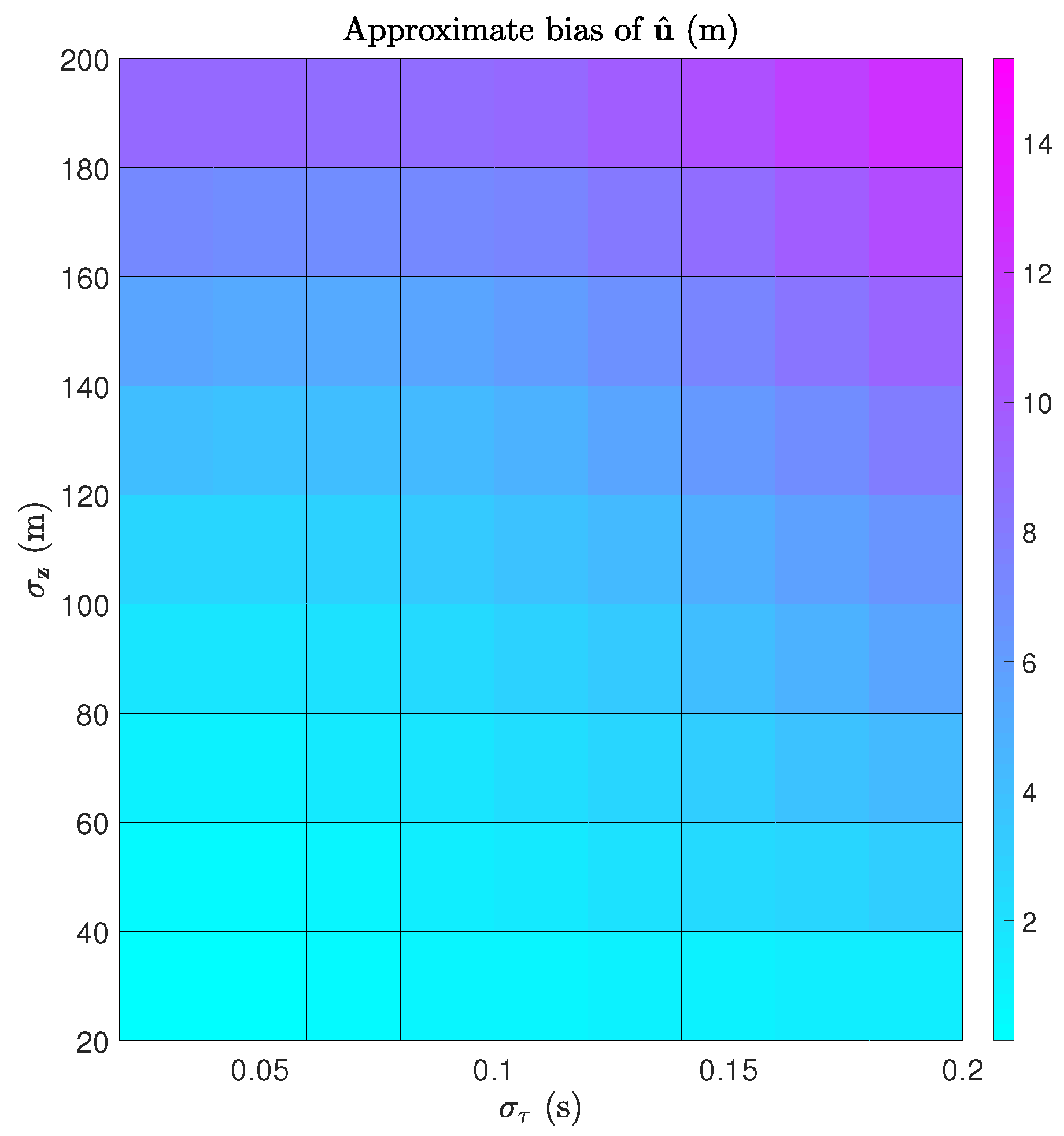
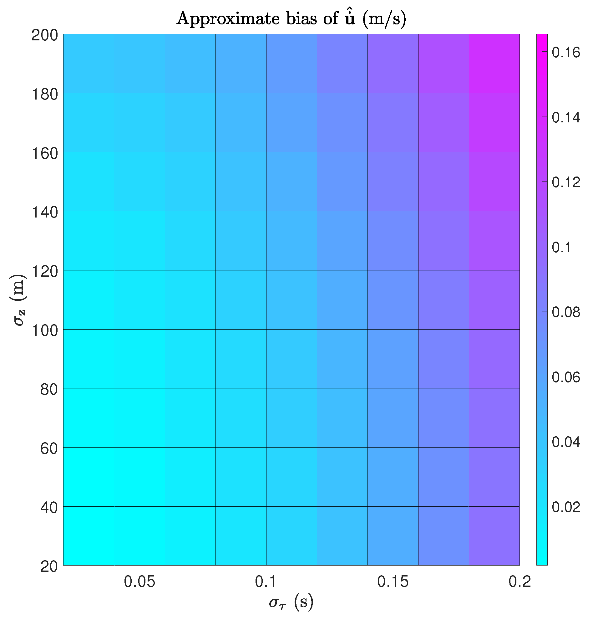
7.2. Bias Calculation

In this subsection, we evaluate the bias of our estimator. The simulation settings are as follows. ${\sigma }_{\tau }$ is from $0.02$ s to $0.2$ s with a step size of $0.02$ s, and ${\sigma }_{\mathbf{z}}$ is from 20 m to 200 m with a step size of 20 m. The norms of the theoretical bias vectors of $\widehat{\mathbf{u}}$ and $\widehat{\dot{\mathbf{u}}}$ are calculated using results from Section 6 and further visualized as surface plots in Figure 5 and Figure 6. It is consistent with intuition that the biases of both $\widehat{\mathbf{u}}$ and $\widehat{\dot{\mathbf{u}}}$ increase with both ${\sigma }_{\tau }$ and ${\sigma }_{\mathbf{z}}$. It should be noted that the biases are relatively small compared with the norms of $\mathbf{u}={[0,2000]}^{\mathrm{T}}$ m and $\dot{\mathbf{u}}={[20,10]}^{\mathrm{T}}$ m/s, even if the noise levels are high, e.g., ${\sigma }_{\tau }=0.2$ s and ${\sigma }_{\mathbf{z}}=200$ m.

Figure 5. Surface plot of norm of the approximate bias of $\widehat{\mathbf{u}}$.

Figure 6. Surface plot of norm of the approximate bias of $\widehat{\dot{\mathbf{u}}}$.

7.3. Localizing Multiple Disjoint Targets

The aim of this section is to evaluate the computational complexity of the algorithm in the sense of scalability, since the WLS algorithm involved in our estimator is computationally efficient. One advantage of our estimator is that it is ready to be extended to location of multiple disjoint targets by concatenating the data matrices in Section 5. Let the number of the disjoint targets be K, and ${10}^3$ Monte Carlo experiments of joint location are performed for each value of $K(=1,2,4,8,16,32,64)$. Then, the running time of the ${10}^3$ experiments are recorded. For convenience of comparison, we normalize the running time for each K with the one for $K=1$. The normalized running times are plotted in Figure 7 using log-log scale. It can be seen that the running time grows almost exponentially with respected to the number of targets. This observation indicates that localizing multiple targets sequentially is more time-efficient than localizing them simultaneously using our estimator. Such defects may root in the fact that our joint estimator does not share the nuisance parameters across the multiple targets.

Figure 7. Normalized running time for locating multiple disjoint targets.

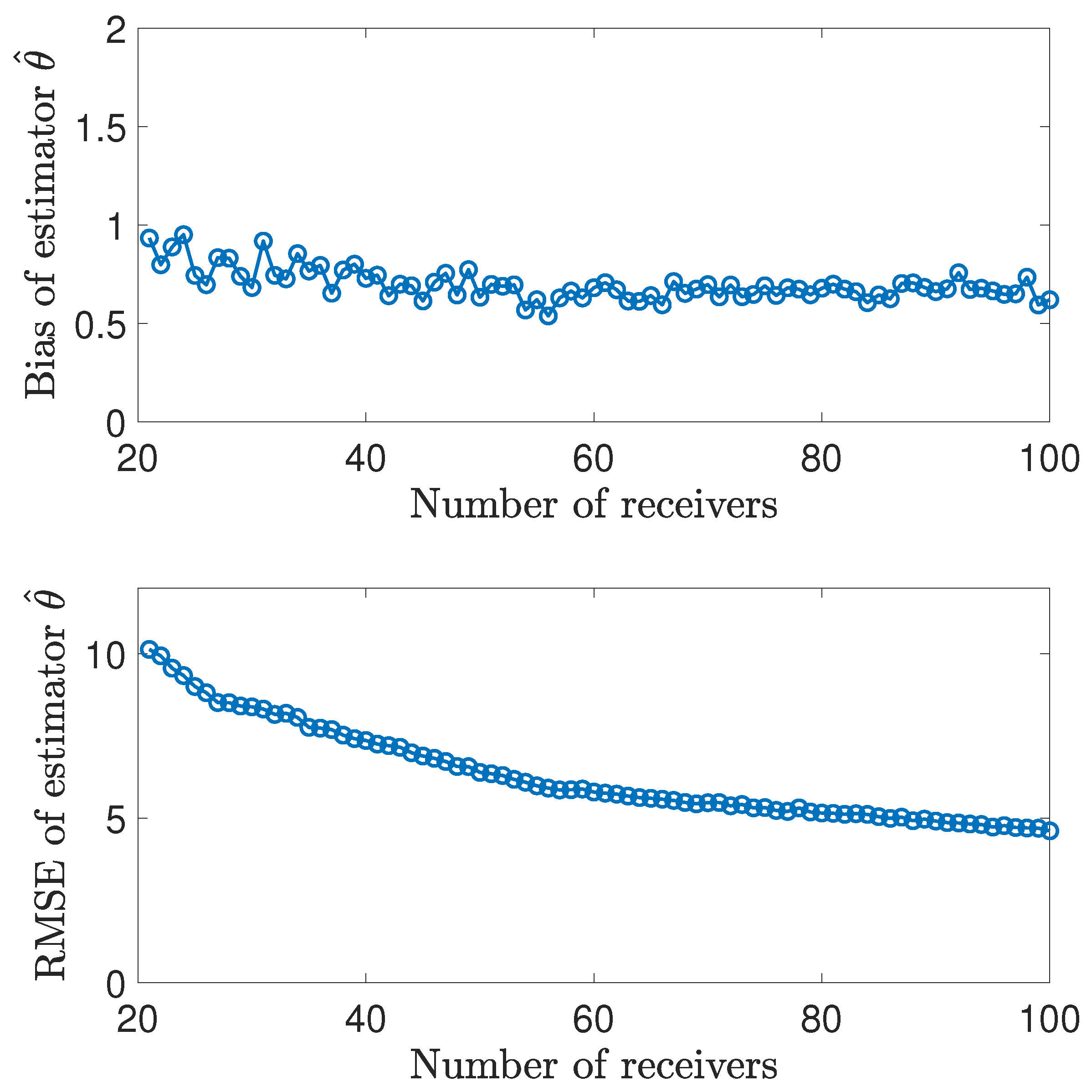
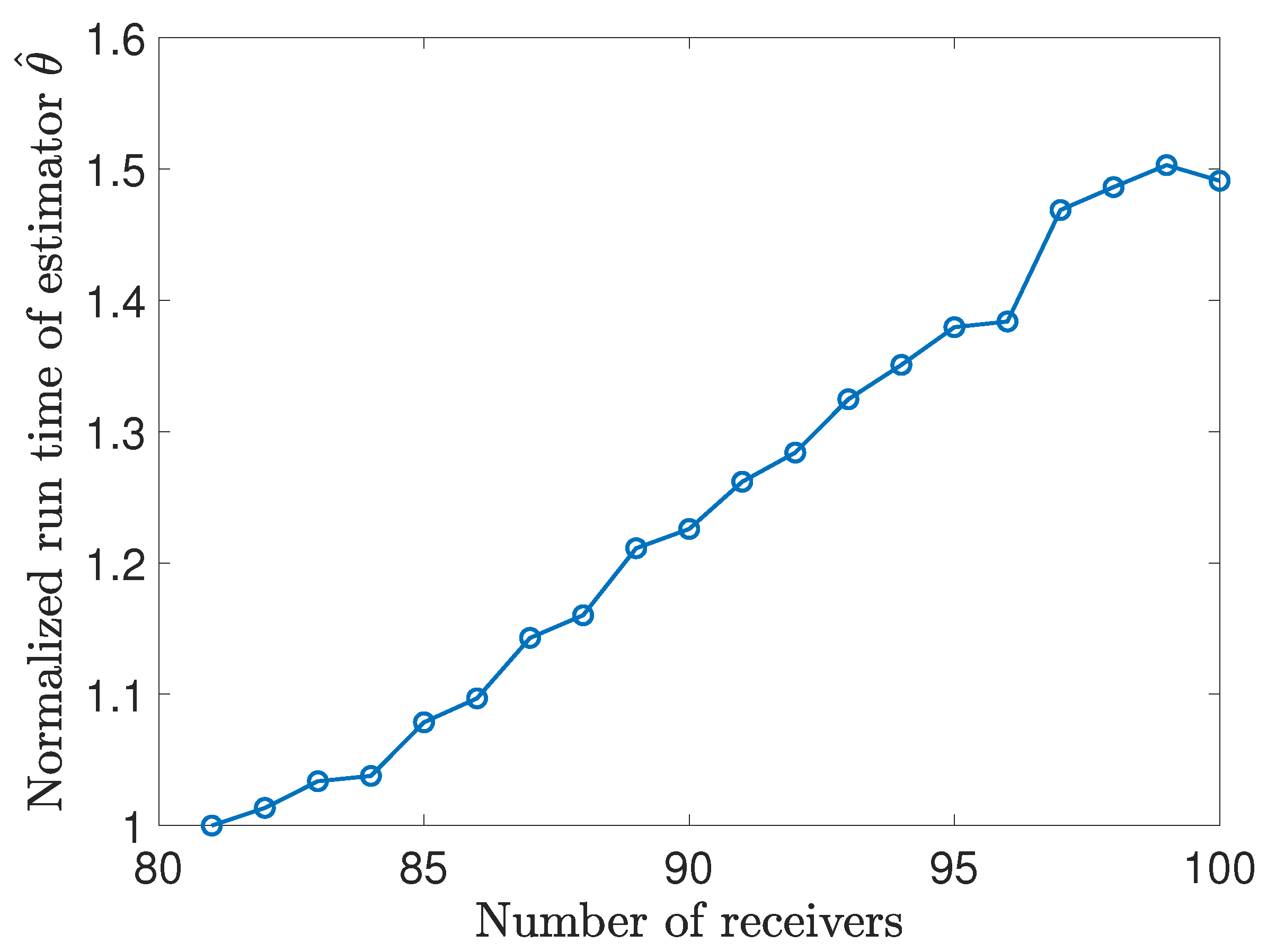
7.4. Large-Scale Simulation Experiments

The location scenario in Section 7.1 through Section 7.3 is the one examined in [6]. In order to evaluate the performance of the proposed estimator more comprehensively, we design the following lareg-scale random experiments. In view of the symmetry of the transmitter ${\mathbf{t}}_i$ and receiver ${\mathbf{s}}_j$ in the observation model, we fix the number of transmitters to 1, and increase the number of receivers from 21 to 100. The transmitter’s position is fixed at ${[0,0]}^{\mathrm{T}}$ m. Both the x-ordinate and y-ordinate of the individual receiver’s position have the uniform probability distribution within the interval ${[-5000,5000]}^{\mathrm{T}}$ m. ${\sigma }_{\mathbf{z}}=20$ m, and ${\sigma }_{\tau }=0.02$ s. Other unspecified settings in these experiments are referred in Table 4. In each location scenario, we conduct ${10}^4$ Monte Carlo simulations. Then we explore the effect of the number of reveivers on the bias/RMSE and computational complexity of the proposed estimator in Figure 8 and Figure 9.

Figure 8. Normalized running time for locating multiple disjoint targets.

Figure 9. Normalized running time for locating multiple disjoint targets.

Figure 8 shows that increasing the number of receivers helps to reduce the RMSE of the estimator. It should be noted that increasing the number of receivers does not lead to a decrease of bias. This fact may imply that designing unbiased estimators is an inherently difficult problem in nonlinear estimation.

In addition, as can be seen in Figure 9, the estimator’s relative running time scales linearly as more receivers are used when the number of the receivers is large enough (e.g., $N>80$ here). This trend coincides with the theoretical linear complexity obtained in Section 6.3.

8. Conclusions

This paper develops a non-iterative solution to the nonlinear hybrid parameter estimation problem of determining the position and velocity of a moving target in a multistatic sonar system in the presence of sensor position uncertainties. It outperforms conventional methods such as SI-TS and TS-WLS in RMSE, and can achieve the HCRB for moderate Gaussian observation noises and sensor position errors. Our estimator involves only two WLS minimizations. Thus, it is computationally efficient, and does not need to deal with the difficulties of initialization and local convergence. Moreover, we obtain the bias vector and covariance matrix of this estimator using perturbation analysis and multivariate statistics.

Appendix A.1. Jacobian Matrix of Target Position and Velocity

$$\frac{\partial \overline{\mathbf{m}}}{\partial \mathit{\theta }}=\left[\begin{array}{cc}\partial {\overline{\mathbf{m}}}_1/\partial \mathbf{u}& \partial {\overline{\mathbf{m}}}_1/\partial \dot{\mathbf{u}}\\ \partial {\overline{\mathbf{m}}}_2/\partial \mathbf{u}& \partial {\overline{\mathbf{m}}}_2/\partial \dot{\mathbf{u}}\\ ⋮& ⋮\\ \partial {\overline{\mathbf{m}}}_M/\partial \mathbf{u}& \partial {\overline{\mathbf{m}}}_M/\partial \dot{\mathbf{u}}\end{array}\right],$$

(A1)

where

$$\begin{array}{ccc}\hfill \frac{\partial {\overline{\mathbf{m}}}_i}{\partial \mathbf{u}}& =& {\left[{\left(\frac{\partial {\tau }_{i,1}^o}{\partial \mathbf{u}}\right)}^{\mathrm{T}},\dots ,{\left(\frac{\partial {\tau }_{i,N}^o}{\partial \mathbf{u}}\right)}^{\mathrm{T}},{\left(\frac{\partial f_{i,1}^o}{\partial \mathbf{u}}\right)}^{\mathrm{T}},\dots ,{\left(\frac{\partial f_{i,N}^o}{\partial \mathbf{u}}\right)}^{\mathrm{T}}\right]}^{\mathrm{T}},\hfill \\ \hfill \frac{\partial {\overline{\mathbf{m}}}_i}{\partial \dot{\mathbf{u}}}& =& {\left[{\left(\frac{\partial {\tau }_{i,1}^o}{\partial \dot{\mathbf{u}}}\right)}^{\mathrm{T}},\dots ,{\left(\frac{\partial {\tau }_{i,N}^o}{\partial \dot{\mathbf{u}}}\right)}^{\mathrm{T}},{\left(\frac{\partial f_{i,1}^o}{\partial \dot{\mathbf{u}}}\right)}^{\mathrm{T}},\dots ,{\left(\frac{\partial f_{i,N}^o}{\partial \dot{\mathbf{u}}}\right)}^{\mathrm{T}}\right]}^{\mathrm{T}},\hfill \end{array}$$

for $i=1,2,\dots ,M$.

$$\begin{array}{ccc}\hfill \partial {\tau }_{i,j}^o/\partial \mathbf{u}& =& \frac{1}{c}{({\rho }_{\mathbf{u},{\mathbf{t}}_i}+{\rho }_{\mathbf{u},{\mathbf{s}}_j})}^{\mathrm{T}},\hfill \\ \hfill \partial {\tau }_{i,j}^o/\partial \dot{\mathbf{u}}& =& {\mathbf{0}}_{1\times 2},\hfill \\ \hfill \partial f_{i,j}^o/\partial \mathbf{u}& =& \frac{1}{c}{\dot{\mathbf{u}}}^{\mathrm{T}}\left({\mathbf{A}}_{\mathbf{u},{\mathbf{t}}_i}+{\mathbf{A}}_{\mathbf{u},{\mathbf{s}}_j}\right),\hfill \\ \hfill \partial f_{i,j}^o/\partial \dot{\mathbf{u}}& =& \frac{1}{c}{({\rho }_{\mathbf{u},{\mathbf{t}}_i}+{\rho }_{\mathbf{u},{\mathbf{s}}_j})}^{\mathrm{T}},\hfill \end{array}$$

for $i=1,2,\dots ,M$ and $j=1,2,\dots ,N$.

Appendix A.2. Jacobian Matrix of Sensor Positions

$$\frac{\partial \overline{\mathbf{m}}}{\partial \mathbf{z}}=\left[\begin{array}{cc}\partial {\overline{\mathbf{m}}}_1/\partial \mathbf{t}& \partial {\overline{\mathbf{m}}}_1/\partial \mathbf{s}\\ \partial {\overline{\mathbf{m}}}_2/\partial \mathbf{t}& \partial {\overline{\mathbf{m}}}_2/\partial \mathbf{s}\\ ⋮& ⋮\\ \partial {\overline{\mathbf{m}}}_M^{/}\partial \mathbf{t}& \partial {\overline{\mathbf{m}}}_M/\partial \mathbf{s}\end{array}\right],$$

(A2)

where

$$\begin{array}{ccc}\hfill \frac{\partial {\overline{\mathbf{m}}}_i}{\partial \mathbf{t}}& =& {\left[{\left(\frac{\partial {\tau }_{i,1}^o}{\partial \mathbf{t}}\right)}^{\mathrm{T}},\dots ,{\left(\frac{\partial {\tau }_{i,N}^o}{\partial \mathbf{t}}\right)}^{\mathrm{T}},{\left(\frac{\partial f_{i,1}^o}{\partial \mathbf{t}}\right)}^{\mathrm{T}},\dots ,{\left(\frac{\partial f_{i,N}^o}{\partial \mathbf{t}}\right)}^{\mathrm{T}}\right]}^{\mathrm{T}},\hfill \\ \hfill \frac{\partial {\overline{\mathbf{m}}}_i}{\partial \mathbf{s}}& =& {\left[{\left(\frac{\partial {\tau }_{i,1}^o}{\partial \mathbf{s}}\right)}^{\mathrm{T}},\dots ,{\left(\frac{\partial {\tau }_{i,N}^o}{\partial \mathbf{s}}\right)}^{\mathrm{T}},{\left(\frac{\partial f_{i,1}^o}{\partial \mathbf{s}}\right)}^{\mathrm{T}},\dots ,{\left(\frac{\partial f_{i,N}^o}{\partial \mathbf{s}}\right)}^{\mathrm{T}}\right]}^{\mathrm{T}},\hfill \end{array}$$

for $i=1,2,\dots ,M$.

$$\begin{array}{ccc}\hfill \partial {\tau }_{i,j}^o/\partial {\mathbf{t}}_k& =& \left\{\begin{array}{cc}{({\rho }_{{\mathbf{t}}_i,\mathbf{u}}-{\rho }_{{\mathbf{t}}_i,{\mathbf{s}}_j})}^{\mathrm{T}}/c,\hfill & \mathrm{if}i=k,\hfill \\ {\mathbf{0}}_{1\times 2},\hfill & \mathrm{if}i\ne k,\hfill \end{array}\right.\hfill \\ \hfill \partial {\tau }_{i,j}^o/\partial {\mathbf{s}}_l& =& \left\{\begin{array}{cc}{({\rho }_{{\mathbf{s}}_j,\mathbf{u}}-{\rho }_{{\mathbf{s}}_j,{\mathbf{t}}_i})}^{\mathrm{T}}/c,\hfill & \mathrm{if}j=l,\hfill \\ {\mathbf{0}}_{1\times 2},\hfill & \mathrm{if}j\ne l,\hfill \end{array}\right.\hfill \\ \hfill \partial f_{i,j}^o/\partial {\mathbf{t}}_k& =& \left\{\begin{array}{cc}-{\dot{\mathbf{u}}}^{\mathrm{T}}{\mathbf{A}}_{{\mathbf{t}}_i,\mathbf{u}}/c,\hfill & \mathrm{if}i=k,\hfill \\ {\mathbf{0}}_{1\times 2},\hfill & \mathrm{if}i\ne k,\hfill \end{array}\right.\hfill \\ \hfill \partial f_{i,j}^o/\partial {\mathbf{s}}_l& =& \left\{\begin{array}{cc}-{\dot{\mathbf{u}}}^{\mathrm{T}}{\mathbf{A}}_{{\mathbf{s}}_j,\mathbf{u}}/c,\hfill & \mathrm{if}j=l,\hfill \\ {\mathbf{0}}_{1\times 2},\hfill & \mathrm{if}j\ne l,\hfill \end{array}\right.\hfill \end{array}$$

for $i=1,2,\dots ,M$, $j=1,2,\dots ,N$, $k=1,2,\dots ,M$ and $l=1,2,\dots ,N$.

Appendix E.1. Formulas for Computing Bias in the First Stage

$$\mathsf{\Delta }{\mathbf{G}}_1={[\mathsf{\Delta }{\mathbf{G}}_{1,1}^{\mathrm{T}},\mathsf{\Delta }{\mathbf{G}}_{1,2}^{\mathrm{T}},\dots ,\mathsf{\Delta }{\mathbf{G}}_{1,M}^{\mathrm{T}}]}^{\mathrm{T}},$$

where for $i=1,2,\dots ,M$,

$$\begin{array}{ccc}\hfill \mathsf{\Delta }{\mathbf{G}}_{1,i}& =& c(2{\mathbf{E}}_{1,i}\delta {\mathbf{e}}_{1,i}+{\mathbf{E}}_{3,i}\delta {\mathbf{e}}_{1,i}+{\mathbf{E}}_{2,i}\delta {\mathbf{e}}_{2,i}),\hfill \\ \hfill {\mathbf{e}}_{1,i}& =& [{\mathbf{0}}_{1\times (i+1)},1,{\mathbf{0}}_{1\times (2M+2-i)}],\hfill \\ \hfill {\mathbf{e}}_{2,i}& =& [{\mathbf{0}}_{1\times (M+i+3)},1,{\mathbf{0}}_{1\times (M-i)}],\hfill \\ \hfill {\mathbf{E}}_{1,i}& =& [{\mathbf{0}}_{2N\times 2(M+iN)},{[{\mathbf{I}}_N,{\mathbf{0}}_N]}^{\mathrm{T}},{\mathbf{0}}_{2N\times [2N(M-i)+N]}],\hfill \\ \hfill {\mathbf{E}}_{2,i}& =& [{\mathbf{0}}_{2N\times 2(M+iN)},{[{\mathbf{0}}_N,{\mathbf{I}}_N]}^{\mathrm{T}},{\mathbf{0}}_{2N\times [2N(M-i)+N]}],\hfill \\ \hfill {\mathbf{E}}_{3,i}& =& [{\mathbf{0}}_{2N\times [2(M+iN)+N]},{[{\mathbf{0}}_N,{\mathbf{I}}_N]}^{\mathrm{T}},{\mathbf{0}}_{2N\times 2N(M-i)}].\hfill \end{array}$$

With some well-known formulas in multivariate statistics and Equation (A15), we list the related expected values as follows, where

$$\mathbf{Q}=blkdiag({\mathbf{Q}}_{\mathbf{z}},{\mathbf{Q}}_{\mathbf{m}}).$$

(A22)

• Let ${\mathbf{K}}_1\left\{i\right\}={\mathbf{K}}_1(2N(i-1)+1:2Ni,:)$ for $i=1,2,\dots ,M$. Then

  $$\begin{array}{cc}\hfill & E[\mathsf{\Delta }{\mathbf{G}}_1^{\mathrm{T}}{\mathbf{K}}_1{\mathbf{B}}_1{ϵ}_1^{(1)}]\hfill \\ \hfill =& \sum _{i=1}^{M}E\left(\mathsf{\Delta }{\mathbf{G}}_{1,i}^{\mathrm{T}}{\mathbf{K}}_1\left\{i\right\}{\mathbf{B}}_1{ϵ}_1^{(1)}\right)\hfill \\ \hfill =& 2c\sum _{i=1}^M{\mathbf{e}}_{1,i}^{\mathrm{T}}tr({\mathbf{E}}_{1,i}^{\mathrm{T}}{\mathbf{K}}_1\left\{i\right\}{\mathbf{B}}_1[{\mathbf{D}}_{\mathbf{z}},c\mathbf{I}]\mathbf{Q})\hfill \\ & +c\sum _{i=1}^M{\mathbf{e}}_{1,i}^{\mathrm{T}}tr({\mathbf{E}}_{3,i}^{\mathrm{T}}{\mathbf{K}}_1\left\{i\right\}{\mathbf{B}}_1[{\mathbf{D}}_{\mathbf{z}},c\mathbf{I}]\mathbf{Q})\hfill \\ & +c\sum _{i=1}^M{\mathbf{e}}_{2,i}^{\mathrm{T}}tr({\mathbf{E}}_{2,i}^{\mathrm{T}}{\mathbf{K}}_1\left\{i\right\}{\mathbf{B}}_1[{\mathbf{D}}_{\mathbf{z}},c\mathbf{I}]\mathbf{Q}).\hfill \end{array}$$
• $$\begin{array}{cc}\hfill & E[\mathsf{\Delta }{\mathbf{G}}_1{\mathbf{H}}_1^o{\mathbf{B}}_1{\mathit{ϵ}}_1^{(1)}]\hfill \\ \hfill =& {[E{[\mathsf{\Delta }{\mathbf{G}}_{1,1}{\mathbf{H}}_1^o{\mathbf{B}}_1{\mathit{ϵ}}_1^{(1)}]}^{\mathrm{T}},\dots ,E{[\mathsf{\Delta }{\mathbf{G}}_{1,M}{\mathbf{H}}_1^o{\mathbf{B}}_1{\mathit{ϵ}}_1^{(1)}]}^{\mathrm{T}}]}^{\mathrm{T}},\hfill \end{array}$$

  where

  $$\begin{array}{cc}\hfill & E[\mathsf{\Delta }{\mathbf{G}}_{1,i}{\mathbf{H}}_1^o{\mathbf{B}}_1{\mathit{ϵ}}_1^{(1)}]\hfill \\ \hfill =& 2c{\mathbf{E}}_{1,i}\mathbf{Q}{({\mathbf{e}}_{1,i}{\mathbf{H}}_1^o{\mathbf{B}}_1[{\mathbf{D}}_{\mathbf{z}},c\mathbf{I}])}^{\mathrm{T}}\hfill \\ & +c{\mathbf{E}}_{3,i}\mathbf{Q}{({\mathbf{e}}_{1,i}{\mathbf{H}}_1^o{\mathbf{B}}_1[{\mathbf{D}}_{\mathbf{z}},c\mathbf{I}])}^{\mathrm{T}}\hfill \\ & +c{\mathbf{E}}_{2,i}\mathbf{Q}{({\mathbf{e}}_{2,i}{\mathbf{H}}_1^o{\mathbf{B}}_1[{\mathbf{D}}_{\mathbf{z}},c\mathbf{I}])}^{\mathrm{T}},\hfill \end{array}$$

  for $i=1,2,\dots ,M$.

Appendix E.2. Formulas for Computing Bias in the Second Stage

$$\begin{array}{ccc}\hfill \mathsf{\Delta }{\mathbf{G}}_2& =& \left[\begin{array}{cc}{\mathbf{0}}_{2\times 2}& {\mathbf{0}}_{2\times 2}\\ {\mathbf{1}}_{M\times 1}\otimes (-2\mathsf{\Delta }{\mathbf{u}}^{\mathrm{T}})& {\mathbf{0}}_{M\times 2}\\ {\mathbf{0}}_{2\times 2}& {\mathbf{0}}_{2\times 2}\\ {\mathbf{1}}_{M\times 1}\otimes (-\mathsf{\Delta }{\dot{\mathbf{u}}}^{\mathrm{T}})& {\mathbf{1}}_{M\times 1}\otimes (-\mathsf{\Delta }{\mathbf{u}}^{\mathrm{T}})\end{array}\right],\hfill \\ \hfill \mathsf{\Delta }{\mathbf{B}}_2& =& \left[\begin{array}{cc}diag([0,0,2\mathsf{\Delta }{\mathit{\alpha }}^{\mathrm{T}}])& {\mathbf{0}}_{(M+2)\times (M+2)}\\ diag([0,0,\mathsf{\Delta }{\mathit{\beta }}^{\mathrm{T}}])& diag([0,0,\mathsf{\Delta }{\mathit{\alpha }}^{\mathrm{T}}])\end{array}\right].\hfill \end{array}$$

All the expected values required for calculating ${\mathit{\mu }}_2$ are listed as follows, where $\mathbf{S}$ is the mean squared error matrix of $\mathsf{\Delta }{\mathit{\varphi }}_1$, i.e.,

$$\mathbf{S}={{\mathbf{P}}_1^o}^{-1}+{\mathit{\mu }}_1{\mathit{\mu }}_1^{\mathrm{T}}.$$

• $$\begin{array}{ccc}\hfill E[{(\mathsf{\Delta }{\alpha }_i)}^2]& \approx & \mathbf{S}(i+2,i+2),i=1,2,\dots ,M,\hfill \\ \hfill E[\mathsf{\Delta }{\alpha }_i\mathsf{\Delta }{\beta }_i]& \approx & \mathbf{S}(i+2,i+M+4),i=1,2,\dots ,M,\hfill \\ \hfill E[\mathsf{\Delta }{\mathbf{u}}^{\mathrm{T}}\mathsf{\Delta }\mathbf{u}]& \approx & tr(\mathbf{S}(1:2,1:2)),\hfill \\ \hfill E[\mathsf{\Delta }{\mathbf{u}}^{\mathrm{T}}\mathsf{\Delta }\dot{\mathbf{u}}]& \approx & tr(\mathbf{S}(1:2,M+3:M+4)).\hfill \end{array}$$
• $$\begin{array}{cc}\hfill & \mathsf{\Delta }{\mathbf{G}}_2{\mathbf{H}}_2^o\hfill \\ =& \left[\begin{array}{c}{\mathbf{0}}_{2\times 1}\\ {\mathbf{1}}_{M\times 1}\otimes (-2\mathsf{\Delta }{\mathbf{u}}^{\mathrm{T}}){\mathbf{H}}_2^o(1:2,:)\\ {\mathbf{0}}_{2\times 1}\\ {\mathbf{1}}_{M\times 1}\otimes (-\mathsf{\Delta }{\dot{\mathbf{u}}}^{\mathrm{T}}){\mathbf{H}}_2^o(1:2,:)+{\mathbf{1}}_{M\times 1}\otimes (-\mathsf{\Delta }{\mathbf{u}}^{\mathrm{T}}){\mathbf{H}}_2^o(3:4,:)\end{array}\right],\hfill \end{array}$$

  where

  $$\begin{array}{ccc}\hfill E[\mathsf{\Delta }{\mathbf{u}}^{\mathrm{T}}{\mathbf{H}}_2^o(1:2,:){\mathbf{B}}_2{\mathit{ϵ}}_2^{(1)}]& =& tr({\mathbf{H}}_2^o(1:2,:){\mathbf{B}}_2\mathbf{S}(:,1:2)),\hfill \\ \hfill E[\mathsf{\Delta }{\dot{\mathbf{u}}}^{\mathrm{T}}{\mathbf{H}}_2^o(1:2,:){\mathbf{B}}_2{\mathit{ϵ}}_2^{(1)}]& =& tr({\mathbf{H}}_2^o(1:2,:){\mathbf{B}}_2\mathbf{S}(:,M+3:M+4)),\hfill \\ \hfill E[\mathsf{\Delta }{\mathbf{u}}^{\mathrm{T}}{\mathbf{H}}_2^o(3:4,:){\mathbf{B}}_2{\mathit{ϵ}}_2^{(1)}]& =& tr({\mathbf{H}}_2^o(3:4,:){\mathbf{B}}_2\mathbf{S}(:,1:2)).\hfill \end{array}$$
• $$\begin{array}{cc}\hfill & \mathsf{\Delta }{\mathbf{B}}_2{\mathbf{B}}_2^{-1}\hfill \\ =& \left[\begin{array}{c}{\mathbf{0}}_{2\times (2M+4)}\\ 2\mathsf{\Delta }{\alpha }_1{\mathbf{B}}_2^{-1}(3,:)\\ 2\mathsf{\Delta }{\alpha }_2{\mathbf{B}}_2^{-1}(4,:)\\ ⋮\\ 2\mathsf{\Delta }{\alpha }_M{\mathbf{B}}_2^{-1}(M+2,:)\\ {\mathbf{0}}_{2\times (2M+4)}\\ \mathsf{\Delta }{\alpha }_1{\mathbf{B}}_2^{-1}(M+5,:)+\mathsf{\Delta }{\beta }_1{\mathbf{B}}_2^{-1}(3,:)\\ \mathsf{\Delta }{\alpha }_2{\mathbf{B}}_2^{-1}(M+6,:)+\mathsf{\Delta }{\beta }_2{\mathbf{B}}_2^{-1}(4,:)\\ ⋮\\ \mathsf{\Delta }{\alpha }_M{\mathbf{B}}_2^{-1}(2M+4,:)+\mathsf{\Delta }{\beta }_M{\mathbf{B}}_2^{-1}(M+2,:)\end{array}\right],\hfill \end{array}$$

  where

  $$\begin{array}{ccc}\hfill E[\mathsf{\Delta }{\alpha }_i{\mathbf{B}}_2^{-1}(i+2,:)\mathbf{U}{\mathbf{B}}_2{\mathit{ϵ}}_2^{(1)}]& =& \mathbf{S}(i+2,:){\mathbf{B}}_2^{\mathrm{T}}{\mathbf{U}}^{\mathrm{T}}{\mathbf{B}}_2^{-1}{(i+2,:)}^{\mathrm{T}},\hfill \\ \hfill E[\mathsf{\Delta }{\alpha }_i{\mathbf{B}}_2^{-1}(i+M+4,:)\mathbf{U}{\mathbf{B}}_2{\mathit{ϵ}}_2^{(1)}]& =& \mathbf{S}(i+2,:){\mathbf{B}}_2^{\mathrm{T}}{\mathbf{U}}^{\mathrm{T}}{\mathbf{B}}_2^{-1}{(i+M+4,:)}^{\mathrm{T}},\hfill \\ \hfill E[\mathsf{\Delta }{\beta }_i{\mathbf{B}}_2^{-1}(i+2,:)\mathbf{U}{\mathbf{B}}_2{\mathit{ϵ}}_2^{(1)}]& =& \mathbf{S}(i+M+4,:){\mathbf{B}}_2^{\mathrm{T}}{\mathbf{U}}^{\mathrm{T}}{\mathbf{B}}_2^{-1}{(i+2,:)}^{\mathrm{T}},\hfill \end{array}$$

  for $i=1,2,\dots ,M$.
• $$\begin{array}{cc}\hfill & \mathsf{\Delta }{\mathbf{G}}_2^{\mathrm{T}}{\mathbf{K}}_2\hfill \\ =& \left[\begin{array}{c}-2\mathsf{\Delta }\mathbf{u}{\sum }_{i=1}^M{\mathbf{K}}_2(i+2,:)-\mathsf{\Delta }\dot{\mathbf{u}}{\sum }_{i=1}^M{\mathbf{K}}_2(i+M+4,:)\\ -\mathsf{\Delta }\mathbf{u}{\sum }_{i=1}^M{\mathbf{K}}_2(i+M+4,:)\end{array}\right],\hfill \end{array}$$

  where

  $$\begin{array}{ccc}\hfill E[\mathsf{\Delta }\mathbf{u}\sum _{i=1}^M{\mathbf{K}}_2(i+2,:){\mathbf{B}}_2{\mathit{ϵ}}_2^{(1)}]& =& \mathbf{S}(1:2,:){\mathbf{B}}_2^{\mathrm{T}}\sum _{i=1}^M{\mathbf{K}}_2{(i+2,:)}^{\mathrm{T}},\hfill \\ \hfill E[(Delta\dot{\mathbf{u}}\sum _{i=1}^M{\mathbf{K}}_2(i+M+4,:){\mathbf{B}}_2{\mathit{ϵ}}_2^{(1)}]& =& \mathbf{S}(M+3:M+4,:){\mathbf{B}}_2^{\mathrm{T}}\sum _{i=1}^M{\mathbf{K}}_2{(i+M+4,:)}^{\mathrm{T}},\hfill \\ \hfill E[\mathsf{\Delta }\mathbf{u}\sum _{i=1}^M{\mathbf{K}}_2(i+M+4,:){\mathbf{B}}_2{\mathit{ϵ}}_2^{(1)}]& =& \mathbf{S}(1:2,:){\mathbf{B}}_2^{\mathrm{T}}\sum _{i=1}^M{\mathbf{K}}_2{(i+M+4,:)}^{\mathrm{T}},\hfill \end{array}$$

  for $i=1,2,\dots ,M$.
• $$\begin{array}{cc}\hfill & \mathsf{\Delta }{\mathbf{B}}_2^{\mathrm{T}}{\mathbf{K}}_2\hfill \\ =& \left[\begin{array}{c}{\mathbf{0}}_{2\times (2M+4)}\\ 2\mathsf{\Delta }{\alpha }_1{\mathbf{K}}_2(3,:)+\mathsf{\Delta }{\beta }_1{\mathbf{K}}_2(M+5,:)\\ 2\mathsf{\Delta }{\alpha }_2{\mathbf{K}}_2(4,:)+\mathsf{\Delta }{\beta }_2{\mathbf{K}}_2(M+6,:)\\ ⋮\\ 2\mathsf{\Delta }{\alpha }_M{\mathbf{K}}_2(M+2,:)+\mathsf{\Delta }{\beta }_M{\mathbf{K}}_2(2M+4,:)\\ {\mathbf{0}}_{2\times (2M+4)}\\ \mathsf{\Delta }{\alpha }_1{\mathbf{K}}_2(M+5,:)\\ \mathsf{\Delta }{\alpha }_2{\mathbf{K}}_2(M+6,:)\\ ⋮\\ \mathsf{\Delta }{\alpha }_M{\mathbf{K}}_2(2M+4,:)\end{array}\right],\hfill \end{array}$$

  where

  $$\begin{array}{ccc}\hfill E[\mathsf{\Delta }{\alpha }_i{\mathbf{K}}_2(i+2,:){\mathbf{B}}_2{\mathit{ϵ}}_2^{(1)}]& =& \mathbf{S}(i+2,:){\mathbf{B}}_2^{\mathrm{T}}{\mathbf{K}}_2{(i+2,:)}^{\mathrm{T}},\hfill \\ \hfill E[\mathsf{\Delta }{\alpha }_i{\mathbf{K}}_2(i+M+4,:){\mathbf{B}}_2{\mathit{ϵ}}_2^{(1)}]& =& \mathbf{S}(i+2,:){\mathbf{B}}_2^{\mathrm{T}}{\mathbf{K}}_2{(i+M+4,:)}^{\mathrm{T}},\hfill \\ \hfill E[\mathsf{\Delta }{\beta }_i{\mathbf{K}}_2(i+M+4,:){\mathbf{B}}_2{\mathit{ϵ}}_2^{(1)}]& =& \mathbf{S}(i+M+4,:){\mathbf{B}}_2^{\mathrm{T}}{\mathbf{K}}_2{(i+M+4,:)}^{\mathrm{T}},\hfill \end{array}$$

  for $i=1,2,\dots ,M$.

References

- Zhang, Y.; Ho, K.C. Multistatic localization in the absence of transmitter position. IEEE Trans. Signal Process. 2019, 67, 4745–4760. [Google Scholar] [CrossRef]
- He, C.; Wang, Y.; Yu, W.; Song, L. Underwater target localization and synchronization for a distributed SIMO sonar with an isogradient SSP and uncertainties in receiver locations. Sensors 2019, 19, 1976. [Google Scholar] [CrossRef] [PubMed]
- Liang, J.; Chen, Y.; So, H.; Jing, Y. Circular/hyperbolic/elliptic localization via Euclidean norm elimination. Signal Process. 2018, 148, 102–113. [Google Scholar] [CrossRef]
- Peters, D.J. A Bayesian method for localization by multistatic active sonar. IEEE J. Ocean. Eng. 2017, 42, 135–142. [Google Scholar] [CrossRef]
- Yang, L.; Yang, L.; Ho, K.C. Moving target localization in multistatic sonar by differential delays and Doppler shifts. IEEE Signal Process. Lett. 2016, 23, 1160–1164. [Google Scholar] [CrossRef]
- Rui, L.; Ho, K.C. Efficient closed-form estimators for multistatic sonar localization. IEEE Trans. Aerosp. Electron. Syst. 2015, 51, 600–614. [Google Scholar] [CrossRef]
- Rui, L.; Ho, K.C. Elliptic localization: Performance study and optimum receiver placement. IEEE Trans. Signal Process. 2014, 62, 4673–4688. [Google Scholar] [CrossRef]
- Ehlers, F.; Ricci, G.; Orlando, D. Batch tracking algorithm for multistatic sonars. IET Radar Sonar Navig. 2012, 6, 746–752. [Google Scholar] [CrossRef]
- Daun, M.; Ehlers, F. Tracking algorithms for multistatic sonar systems. EURASIP J. Adv. Signal Process. 2010, 2010, 461538. [Google Scholar] [CrossRef]
- Simakov, S. Localization in airborne multistatic sonars. IEEE J. Ocean. Eng. 2008, 33, 278–288. [Google Scholar] [CrossRef]
- Coraluppi, S. Multistatic sonar localization. IEEE J. Ocean. Eng. 2006, 31, 964–974. [Google Scholar] [CrossRef]
- Coraluppi, S.; Carthel, C. Distributed tracking in multistatic sonar. IEEE Trans. Aerosp. Electron. Syst. 2005, 41, 1138–1147. [Google Scholar] [CrossRef]
- Sandys-Wunsch, M.; Hazen, M.G. Multistatic localization error due to receiver positioning errors. IEEE J. Ocean. Eng. 2002, 27, 328–334. [Google Scholar] [CrossRef]
- Shin, H.; Chung, W. Target localization using double-sided bistatic range measurements in distributed MIMO radar systems. Sensors 2019, 19, 2524. [Google Scholar] [CrossRef]
- Amiri, R.; Behnia, F.; Noroozi, A. Efficient algebraic solution for elliptic target localisation and antenna position refinement in multiple-input–multiple-output radars. IET Radar Sonar Navig. 2019, 13, 2046–2054. [Google Scholar] [CrossRef]
- Amiri, R.; Behnia, F.; Noroozi, A. Efficient joint moving target and antenna localization in distributed MIMO radars. IEEE Trans. Wirel. Commun. 2019, 18, 4425–4435. [Google Scholar] [CrossRef]
- Amiri, R.; Behnia, F.; Zamani, H. Asymptotically efficient target localization from bistatic range measurements in distributed MIMO radars. IEEE Signal Process. Lett. 2017, 24, 299–303. [Google Scholar] [CrossRef]
- Einemo, M.; So, H.C. Weighted least squares algorithm for target localization in distributed MIMO radar. Signal Process. 2015, 115, 144–150. [Google Scholar] [CrossRef]
- Dianat, M.; Taban, M.R.; Dianat, J.; Sedighi, V. Target localization using least squares estimation for MIMO radars with widely separated antennas. IEEE Trans. Aerosp. Electron. Syst. 2013, 49, 2730–2741. [Google Scholar] [CrossRef]
- Godrich, H.; Haimovich, A.M.; Blum, R.S. Target localization accuracy gain in MIMO radar-based systems. IEEE Trans. Inf. Theory 2010, 56, 2783–2803. [Google Scholar] [CrossRef]
- Zhao, Y.; Hu, D.; Zhao, Y.; Liu, Z.; Zhao, C. Refining inaccurate transmitter and receiver positions using calibration targets for target localization in multi-static passive radar. Sensors 2019, 19, 3365. [Google Scholar] [CrossRef] [PubMed]
- Wang, J.; Qin, Z.; Wei, S.; Sun, Z.; Xiang, H. Effects of nuisance variables selection on target localisation accuracy in multistatic passive radar. Electron. Lett. 2018, 54, 1139–1141. [Google Scholar] [CrossRef]
- Chalise, B.K.; Zhang, Y.D.; Amin, M.G.; Himed, B. Target localization in a multi-static passive radar system through convex optimization. Signal Process. 2014, 102, 207–215. [Google Scholar] [CrossRef]
- Gorji, A.A.; Tharmarasa, R.; Kirubarajan, T. Widely separated MIMO versus multistatic radars for target localization and tracking. IEEE Trans. Aerosp. Electron. Syst. 2013, 49, 2179–2194. [Google Scholar] [CrossRef]
- Malanowski, M.; Kulpa, K. Two methods for target localization in multistatic passive radar. IEEE Trans. Aerosp. Electron. Syst. 2012, 48, 572–580. [Google Scholar] [CrossRef]
- Yin, Z.; Jiang, X.; Yang, Z.; Zhao, N.; Chen, Y. WUB-IP: A high-precision UWB positioning scheme for ndoor multiuser applications. IEEE Syst. J. 2019, 13, 279–288. [Google Scholar] [CrossRef]
- Zhou, Y.; Law, C.L.; Guan, Y.L.; Chin, F. Indoor elliptical localization based on asynchronous UWB range measurement. IEEE Trans. Instrum. Meas. 2011, 60, 248–257. [Google Scholar] [CrossRef]
- Smith, J.O.; Abel, J.S. Closed-form least-squares source location estimation from range-difference measurements. IEEE Trans. Acoust. Speech Signal Process. 1987, 35, 1661–1669. [Google Scholar] [CrossRef]
- Schau, H.; Robinson, A. Passive source localization employing intersecting spherical surfaces from time-of-arrival differences. IEEE Trans. Acoust. Speech Signal Process. 1987, 35, 1223–1225. [Google Scholar] [CrossRef]
- Amiri, R.; Behnia, F.; Sadr, M.A.M. Exact solution for elliptic localization in distributed MIMO radar systems. IEEE Trans. Veh. Technol. 2018, 67, 1075–1086. [Google Scholar] [CrossRef]
- Chan, Y.T.; Ho, K.C. A simple and efficient estimator for hyperbolic location. IEEE Trans. Signal Process. 1994, 42, 1905–1915. [Google Scholar] [CrossRef]
- Zheng, B.; Yang, Z. Perturbation analysis for mixed least squares–total least squares problems. Numer. Linear Algebra Appl. 2019, 26, e2239. [Google Scholar] [CrossRef]
- Buranay, S.C.; Iyikal, O.C. A predictor-corrector iterative method for solving linear least squares problems and perturbation error analysis. J. Inequal. Appl. 2019, 2019, 203. [Google Scholar] [CrossRef]
- Xie, P.; Xiang, H.; Wei, Y. A contribution to perturbation analysis for total least squares problems. Numer. Algorithms 2017, 75, 381–395. [Google Scholar] [CrossRef]
- Harville, D.A. Linear Models and the Relevant Distributions and Matrix Algebra; CRC Press: Boca Raton, FL, USA, 2018. [Google Scholar]
- Bar, S.; Tabrikian, J. The risk-unbiased Cramér–Rao bound for non-Bayesian multivariate parameter estimation. IEEE Trans. Signal Process. 2018, 66, 4920–4934. [Google Scholar] [CrossRef]
- Bergel, I.; Noam, Y. Lower bound on the localization error in infinite networks with random sensor locations. IEEE Trans. Signal Process. 2018, 66, 1228–1241. [Google Scholar] [CrossRef]
- Messer, H. The hybrid Cramér–Rao lower bound—From practice to theory. In Proceedings of the 4th IEEE Sensor Array and Multichannel Signal Processing Workshop, Waltham, MA, USA, 12–14 July 2006; pp. 304–307. [Google Scholar] [CrossRef]
- Noam, Y.; Messer, H. The hybrid Cramér–Rao bound and the generalized Gaussian linear estimation problem. In Proceedings of the 5th IEEE Sensor Array and Multichannel Signal Processing Workshop, Darmstadt, Germany, 21–23 July 2008; pp. 395–399. [Google Scholar] [CrossRef]
- Van Trees, H.L.; Bell, K.L.; Tian, Z. Detection, Estimation, and Modulation Theory Part I: Detection, Estimation, and Filtering Theory; John Wiley & Sons: Hoboken, NJ, USA, 2013. [Google Scholar]
- Rockah, Y.; Schultheiss, P. Array shape calibration using sources in unknown locations—Part I: far-field sources. IEEE Trans. Acoust. Speech Signal Process. 1987, 35, 286–299. [Google Scholar] [CrossRef]
- Magnus, J.R.; Neudecker, H. Matrix Differential Calculus with Applications in Statistics and Econometrics; John Wiley & Sons: Hoboken, NJ, USA, 2007. [Google Scholar]
- Chui, C.K.; Chen, G. Kalman Filtering with Real-Time Applications; Springer International Publishing: Berlin/Heidelberg, Germany, 2017. [Google Scholar]
- Li, X.; Wang, S.; Cai, Y. Tutorial: Complexity analysis of Singular Value Decomposition and its variants. arXiv 2019, arXiv:1906.12085. [Google Scholar]
- Foy, W.H. Position-location solutions by Taylor-series estimation. IEEE Trans. Aerosp. Electron. Syst. 1976, 12, 187–194. [Google Scholar] [CrossRef]
- Horn, R.A.; Johnson, C.R. Matrix Analysis, 2nd ed.; Cambridge University Press: Cambridge, UK, 2013. [Google Scholar]
© 2020 by the authors. Licensee MDPI, Basel, Switzerland. This article is an open access article distributed under the terms and conditions of the Creative Commons Attribution (CC BY) license (http://creativecommons.org/licenses/by/4.0/).