New Improvement of the Domain of Parameters for Newton’s Method

Abstract

There is a need to extend the convergence domain of iterative methods for computing a locally unique solution of Banach space valued operator equations. This is because the domain is small in general, limiting the applicability of the methods. The new idea involves the construction of a tighter set than the ones used before also containing the iterates leading to at least as tight Lipschitz parameters and consequently a finer local as well as a semi-local convergence analysis. We used Newton’s method to demonstrate our technique. However, our technique can be used to extend the applicability of other methods too in an analogous manner. In particular, the new information related to the location of the solution improves the one in previous studies. This work also includes numerical examples that validate the proven results.

1. Introduction

Consider, approximating a locally unique solution $z^{*}$ of a nonlinear equation

$$F\left(z\right)=0,$$

(1)

such that F is defined on a convex subset D of a Banach space $B_1$ with values in a Banach space $B_2$ and is a Fréchet–differentiable operator.

The study of numerous problems in diverse areas such as Mathematics, Mathematical: Biology, Chemistry, Economics, Physics, Environmental Sciences, and Engineering to mention a few leads to finding a solution of some equation involving abstract space valued operators. The difficulty in finding a solution of such equation in a closed form focuses us to resort to the development of iterative methods. However, the convergence domain of these methods is small in general for the semi-local as well as the local convergence case. In the case of the widely used Newton’s method, several attempts have been made starting with the seminal work by Kantorovich [1] and continuing with the works by others [1,2,3,4,5,6,7,8,9,10,11,12,13,14,15,16,17,18,19,20,21].

All are trying to extend the convergence domain using Lipschitz type conditions on the operator F’ and starting close enough to the solution $z^{*}$. We refer the reader to the sufficient convergence criteria (3)–(7) for a background. The novelty of our paper is that we further extend the applicability of Newton’s method by introducing a more precise set than in earlier studies containing the using criteria (3)–(7). Then, in this new set, the Lispchitz constants are tighter, resulting in the following advantages $\left(A\right)$ over the earlier works:

$\left(A_1\right)$

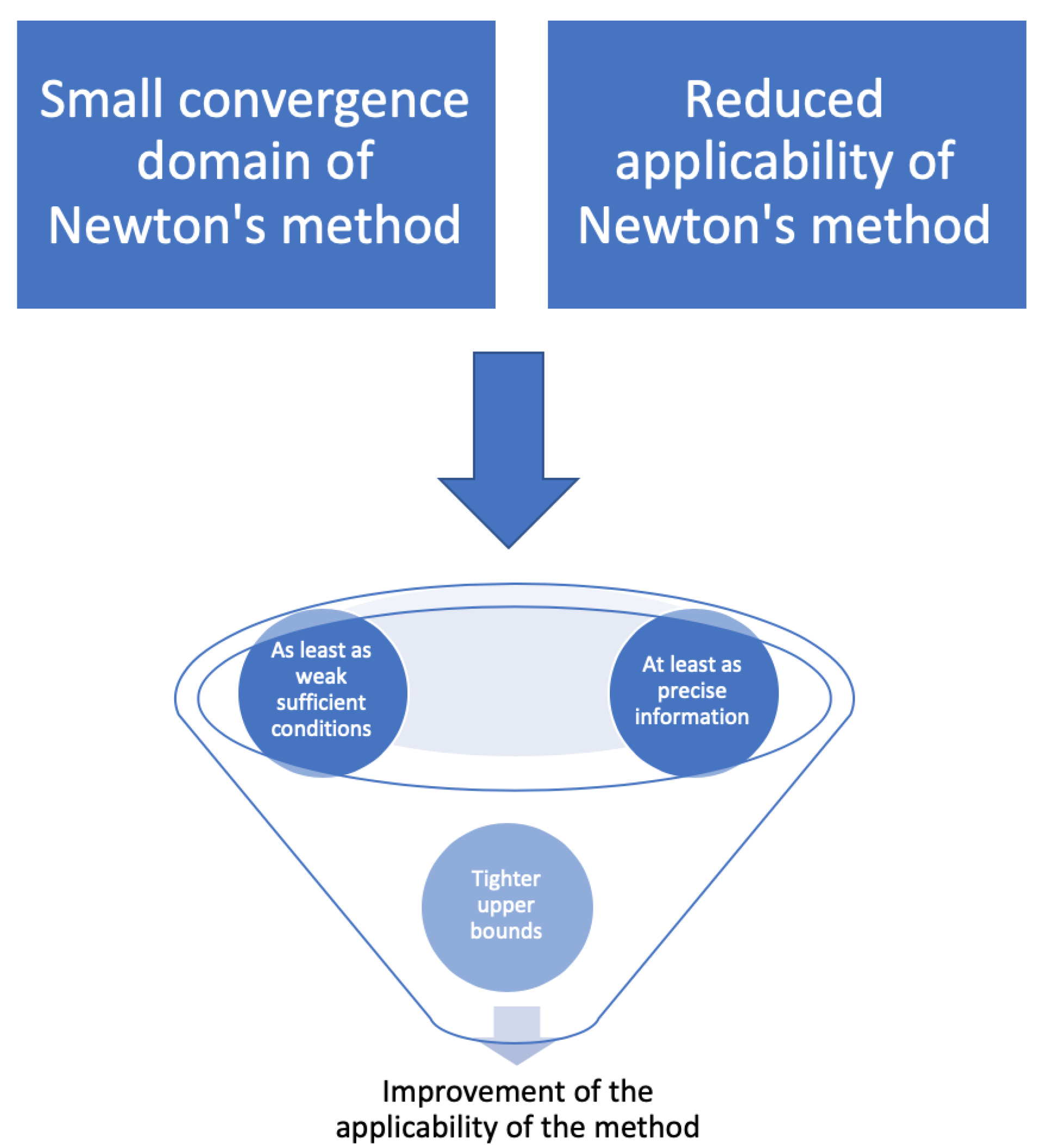
At least as weak sufficient semi-local and local convergence criteria (leading to more initial points)

$\left(A_2\right)$

Tighter upper bounds on the distances $\parallel z_{n+1}-z_n\parallel$ and $\parallel z_n-z^{*}\parallel$ (leading to fewer iterations to obtain a predetermine accuracy)

$\left(A_3\right)$

At least as precise information on the location of the solution.

The advantages $\left(A\right)$ are not arrived at under additional conditions because in practice the new Lipschitz constants are special cases of the old ones, see Figure 1.

Moreover, in advanced mathematics, we need to use different alternatives since we all know the different problems that students present [22,23,24,25,26,27].

It can also be easily seen that our technique can be used to extend the applicability of other methods along the same lines.

Newton’s method for each $n\ge 0$ is defined by

$$z_{n+1}=z_n-F^{\prime }{\left(z_n\right)}^{-1}F\left(z_n\right)$$

(2)

such that $z_0$ is an initial point. This is the most common methodology for approximating $z^{*}$ generating a sequence $\left\{z_n\right\}$. Define open and closed balls $B(z,\varrho )$, $\overline{B}(z,\varrho )$ in $B_1$ with radius $\varrho >0$ and center $z\in B_1$.

The Newton–Kantorovich Theorem [1] is the most reputable semi-local convergence result for Newton’s method using the hypotheses:

Hypothesis 1

($H_1$). There exists $z_0\in D$ with $F^{\prime }{\left(z_0\right)}^{-1}\in L(B_2,B_1)$ and a parameter $\eta \ge 0$ such that

$$\parallel F^{\prime }{\left(z_0\right)}^{-1}F\left(z_0\right)\parallel \le \eta .$$

Hypothesis 2

($H_2$). There exists a parameter $L>0$ and, for each $z,z^1\in D$ such that

$$\parallel F^{\prime }{\left(z_0\right)}^{-1}(F^{\prime }\left(z\right)-F^{\prime }\left(z^1\right))\parallel \le L\parallel z-z^1\parallel$$

and

Hypothesis 3

($H_3$). There exists a closed ball $\overline{B}(z_0,R)\subseteq D$ for some $R>0$.

The renowned and well known Kantorovich hypothesis is based on the sufficient convergence criterion

$$h=2L\eta \le 1.$$

(3)

Commonly, the convergence domain of Newton’s method is based on the parameters L and $\eta$ being small. In order to enlarge the convergence domain, Argyros et al. [7,8] provide sufficient convergence criteria for Newton’s method based on improvements and more precise sequences than before [1,19].

The new conditions are:

$$h_1=2C_1\eta \le 1,$$

(4)

$$h_2=2C_2\eta \le 1,$$

(5)

$$h_3=2C_3\eta \le 1,$$

(6)

$$h_4=2C_4\eta \le 1,$$

(7)

where

$$C_1={\displaystyle \frac{A_0+L}{2}},C_2={\displaystyle \frac{1}{8}}\left(L+4A_0+\sqrt{L^2+8A_{0}L}\right),$$

$$C_3={\displaystyle \frac{1}{8}}\left(4A_0+\sqrt{A_{0}L+8A_0^2}+\sqrt{A_{0}L}\right),C_4={\displaystyle \frac{1}{{\eta }_0}},$$

such that the small positive root of a quadratic polynomial [5,6,7,8] is ${\eta }_0$ and $A_0>0$ is the center Lipschitz constant, where

$$\parallel F^{\prime }{\left(z_0\right)}^{-1}(F^{\prime }\left(x\right)-F^{\prime }\left(z_0\right))\parallel \le A_0\parallel x-z_0\parallel \mathrm{for}\mathrm{each}x\in D,$$

(8)

whose existence is always implied by $\left(H_2\right)$. We have that

$$A_0\le L$$

(9)

is true and $\frac{L}{A_0}$ can be randomly large [7]. Notice that condition (8) is not an added $\left(H_2\right)$ hypothesis, since in practice the computation of parameter L implies the computation of $A_0$ as a special case. Keep in mind that, if $A_0=L$, conditions (4)–(7) reduce to criterion (3). However, if $A_0<L$, we have [7,8]

$$h\le 1\Rightarrow h_1\le 1\Rightarrow h_2\le 1\Rightarrow h_3\le 1\Rightarrow h_4\le 1,$$

(10)

$$\begin{array}{c}{\displaystyle \frac{h_1}{h}}\to {\displaystyle \frac{1}{2}},{\displaystyle \frac{h_2}{h}}\to {\displaystyle \frac{1}{4}},{\displaystyle \frac{h_2}{h_1}}\to {\displaystyle \frac{1}{2}},{\displaystyle \frac{h_3}{h}}\to 0\hfill \end{array}$$

(11)

and

$$\begin{array}{c}{\displaystyle \frac{h_3}{h_2}}\to 0,{\displaystyle \frac{h_3}{h_1}}\to 0,\mathrm{as}{\displaystyle \frac{A_0}{L}}\to 0.\hfill \end{array}$$

(12)

The main findings of this study are related to the distance involved and the improvement of the semi-local criteria (3)–(7) using parameters tighter than $A_0$ and L and restricting the domain. Similar ideas are used to improve error limits and expand radius convergence in the case of the local convergence.

The document is divided as follows: In Section 2 the results of the local and semi-local convergence are presented. In Section 3, we conclude with numerical examples, and, in the final section, we provide the conclusions.

2. Convergence Analysis

To begin, we analyze the semi-local convergence analysis of Newton’s method. Next, a new version of the Newton–Kantorovich Theorem [1] is stated in Theorem 2, whereas, in Theorem 1, we state the Newton–Kantorovich theorem for comparison purposes.

Theorem 1.

Suppose conditions $\left(H_1\right)$–$\left(H_3\right)$ and (3) are verified. Then, the sequence $\left\{z_n\right\}$ is well defined by Newton’s method for each $n\ge 0$, belongs in the ball $B(z_0,R)$, and converges to a unique solution $z^{*}\in \overline{B}(z_0,R)$ of Equation (1), where

$$R={\displaystyle \frac{1-\sqrt{1-h}}{L}}.$$

Next, we state a semi-local convergence result improving the Kantorovich Theorem.

Theorem 2.

Suppose that there exist $z_0\in D$, $\eta \ge 0$, $\gamma \ge 1$, and $A_{\gamma }>0$, such that

$$F^{\prime }{\left(z_0\right)}^{-1}\in L(B_2,B_1),$$

$$\parallel F^{\prime }{\left(z_0\right)}^{-1}F\left(z_0\right)\parallel \le \eta ,$$

$$D_{\gamma }=\overline{B}(z_0,\gamma \eta )\subseteq D,$$

$$\parallel F^{\prime }{\left(z_0\right)}^{-1}(F^{\prime }\left(x\right)-F^{\prime }\left(y\right))\parallel \le A_{\gamma }\parallel x-y\parallel foreachx,y\in D_{\gamma },$$

$$h_{\gamma }=2A_{\gamma }\eta \le 1$$

and

$$R_{\gamma }\le \gamma \eta ,$$

where

$$R_{\gamma }={\displaystyle \frac{1-\sqrt{1-h_{\gamma }}}{A_{\gamma }}}·$$

Then, the sequence $\left\{z_n\right\}$ is well defined by Newton’s method for each $n\ge 0$, belong in a ball $B(z_0,R_{\gamma })$, and converge to a unique solution $z^{*}\in \overline{B}(z_0,R_{\gamma })$ of Equation (1).

Proof. 

The hypotheses $\left(H\right)$ of Theorem 1 are verified immediately on $D_{\gamma }$, if $\overline{B}(z_0,R),L,h,R$ are replaced by $D_{\gamma }$, $A_{\gamma }$, $h_{\gamma }$ and $R_{\gamma }$, respectively. □

Next, we need to introduce an alternative to condition ($H_2$):

Hypothesis 2’

$\left(H_2^{\prime }\right)$. For each $x,y\in B\left(z_0,\frac{1}{A_0}\right)\cap D:=D_1$, there exists a parameter$M>0$

$$\parallel F^{\prime }{\left(z_0\right)}^{-1}(F^{\prime }\left(x\right)-F^{\prime }\left(y\right))\parallel \le M\parallel x-y\parallel .$$

Notice that $M\le L$ holds in general.

Next, we consider criterion (6) and improve a semi-local result given in [7].

Theorem 3.

Suppose that condition (6) and conditions $\left(H_1\right),\left(H_2^{\prime }\right)$ and $\left(H_3\right)$ are verified with

$$r_3=\eta +{\displaystyle \frac{A_0{\eta }^2}{2(1-\alpha )(1-A_0\eta )}},$$

and

$$\alpha ={\displaystyle \frac{2M}{M+\sqrt{M^2+8A_{0}M}}}·$$

Then, the sequence $\left\{z_n\right\}$ is well defined by Newton’s method for each $n\ge 0$, belongs in the ball $B(z_0,r_3)$, and converges to a unique solution $z^{*}\in \overline{B}(z_0,r_3)$ of Equation (1).

Proof. 

It follows by simply noticing that the iterates are such that $z_n\in D_1$, which is a more precise location than D used in previous works leading to $M\le L$ ($D_1\subseteq D$). Then, the proof is analogous to the corresponding in Theorem 2 with M replacing L. □

The next theorem improves the result of Theorem 3.

Theorem 4.

Suppose that there exist $z_0\in D$, $\eta \ge 0$, $\gamma \ge 1$, $M_{\gamma }>0$ and $A_{0,\gamma }\ge 0$ such that

$$F^{\prime }{\left(z_0\right)}^{-1}\in L(B_2,B_1),$$

$$\parallel F^{\prime }{\left(z_0\right)}^{-1}F\left(z_0\right)\parallel \le \eta ,$$

$$D_{\gamma }\subseteq D,$$

$$\parallel F^{\prime }{\left(z_0\right)}^{-1}(F^{\prime }\left(x\right)-F^{\prime }\left(z_0\right))\parallel \le A_{0,\gamma }\parallel x-z_0\parallel foreachx\in D_{\gamma },$$

$$\parallel F^{\prime }{\left(z_0\right)}^{-1}(F^{\prime }\left(x\right)-F^{\prime }\left(y\right))\parallel \le M_{\gamma }\parallel x-y\parallel foreachx,y\in D_{0,\gamma }:=D_{\gamma }\cap B(z_0,\frac{1}{A_{0,\gamma }}),$$

$$h_{3,\gamma }=2A_{3,\gamma }\eta \le 1,$$

and

$$r_{3,\gamma }\le \gamma \eta ,$$

where

$$A_{3,\gamma }={\displaystyle \frac{1}{8}}\left(4A_{0,\gamma }+\sqrt{M_{\gamma }{A}_{0,\gamma }+8A_{0,\gamma }^2}+\sqrt{A_{0,\gamma }{M}_{\gamma }}\right),$$

$$r_{3,\gamma }=\eta +{\displaystyle \frac{A_{0,\gamma }{\eta }^2}{2(1-{\alpha }_{\gamma })(1-A_{0,\gamma }\eta )}},$$

and

$${\alpha }_{\gamma }={\displaystyle \frac{2M_{\gamma }}{M_{\gamma }+\sqrt{M_{\gamma }^2+8A_{0,\gamma }{M}_{\gamma }}}}·$$

Then, the sequence $\left\{z_n\right\}$ is well defined by Newton’s method for each $n\ge 0$, belongs in the ball $B(z_0,r_{3,\gamma })$, and converges to a unique solution $z^{*}\in \overline{B}(z_0,r_{3,\gamma })$ of Equation (1).

Proof. 

The result follows immediately from Theorem 2, if we replace $D_{\gamma }$, $A_{\gamma }$, $h_{\gamma }$, $R_{\gamma }$ by $D_{0,\gamma }$, $A_{0,\gamma }$, $h_{3,\gamma }$ and $r_{3,\gamma }$, respectively. □

Next, we consider criterion (7) and present a semi-local improving the convergence result of Newton’s method given in [8].

Theorem 5.

Suppose that conditions $\left(H_1\right),\left(H_2\right),\left(H_2^{\prime }\right),\left(H_3\right)$, (8) and $D_{\gamma }\subset D$ are verified, and there exist $K_0>0$, $K>0$ such that

$$\parallel F^{\prime }{\left(z_0\right)}^{-1}(F^{\prime }\left(z_1\right)-F^{\prime }\left(z_0\right))\parallel \le K_0\parallel z_1-z_0\parallel ,$$

$$\parallel F^{\prime }{\left(z_0\right)}^{-1}(F^{\prime }(z_0+\theta (z_1-z_0))-F^{\prime }\left(z_0\right))\parallel \le K\theta \parallel z_1-z_0\parallel foreach\theta \in [0,1],$$

$$h_4=2A_4\eta \le 1,$$

where

$$z_1=z_0-F^{\prime }{\left(z_0\right)}^{-1}F\left(z_0\right),$$

$$A_4={\displaystyle \frac{1}{2{\eta }_0}}\le 1,$$

$${\alpha }_0={\displaystyle \frac{L(t_2-t_1)}{2(1-A_0{t}_2)}},$$

$$t_1=\eta ,t_2=\eta +{\displaystyle \frac{K{\eta }^2}{2(1-K_0\eta )}},$$

$$r_4=\eta +\left(1+{\displaystyle \frac{{\alpha }_0}{1-\alpha }}\right){\displaystyle \frac{K{\eta }^2}{2(1-K_0\eta )}}.$$

${\eta }_0$ is defined by

$${\eta }_0=\left\{\begin{array}{cc}{\displaystyle \frac{1}{A_0+K_0}},\hfill & ifB=LK+2\alpha \left(A_0(K-2K_0)\right)=0,\hfill \\ positiverootofp,\hfill & ifB>0,\hfill \\ smallpositiverootofp,\hfill & ifB<0,\hfill \end{array}\right.$$

and

$$p\left(t\right)=(LK+2\alpha A_0(K-2K_0))t^2+4\alpha (A_0+K_0)t-4\alpha .$$

Then, the sequence $\left\{z_n\right\}$ is well defined by Newton’s method for each $n\ge 0$, belongs in a ball $B(z_0,r_4)$, and converges to a unique solution $z^{*}\in \overline{B}(z_0,r_4)$ of Equation (1).

Proof. 

As in the proof below Theorem 2. □

The next theorem improves the result of Theorem 5.

Theorem 6.

Suppose that there exist $z_0\in D$, $\eta \ge 0$, $\gamma \ge 1$, $K_{0,\gamma }>0$, $K_{\gamma }>0$, $M_{\gamma }>0$, and $A_{0,\gamma }\ge 0$ such that

$$F^{\prime }{\left(z_0\right)}^{-1}\in L(B_2,B_1),$$

$$\parallel F^{\prime }{\left(z_0\right)}^{-1}F\left(z_0\right)\parallel \le \eta ,$$

$$D_{\gamma }\subseteq D,$$

$$\parallel F^{\prime }{\left(z_0\right)}^{-1}(F^{\prime }\left(z_1\right)-F^{\prime }\left(z_0\right))\parallel \le K_{0,\gamma }\parallel z_1-z_0\parallel ,$$

$$\parallel F^{\prime }{\left(z_0\right)}^{-1}(F^{\prime }(z_0+\theta (z_1-z_0))-F^{\prime }\left(z_0\right))\parallel \le K_{\gamma }\theta \parallel z_1-z_0\parallel foreach\theta \in [0,1],$$

$$\parallel F^{\prime }{\left(z_0\right)}^{-1}(F^{\prime }\left(x\right)-F^{\prime }\left(z_0\right))\parallel \le A_{0,\gamma }\parallel x-z_0\parallel foreachx\in D_{\gamma },$$

$$\parallel F^{\prime }{\left(z_0\right)}^{-1}(F^{\prime }\left(x\right)-F^{\prime }\left(y\right))\parallel \le M_{\gamma }\parallel x-y\parallel foreachx,y\in D_{1,\gamma }:=D_{\gamma }\cap B\left(z_0,\frac{1}{A_{0,\gamma }}\right),$$

$$h_{4,\gamma }=2A_{4,\gamma }\eta \le 1,$$

and

$$r_{4,\gamma }\le \gamma \eta ,$$

where

$$z_1=z_0-F^{\prime }{\left(z_0\right)}^{-1}F\left(z_0\right),$$

$${\alpha }_{0,\gamma }={\displaystyle \frac{M_{\gamma }(t_2-t_1)}{2(1-A_{0,\gamma }{t}_2)}},$$

$$t_1=\eta ,t_2=\eta +{\displaystyle \frac{K_{\gamma }{\eta }^2}{2(1-K_{0,\gamma }\eta )}},$$

$$r_{4,\gamma }=\eta +\left(1+{\displaystyle \frac{{\alpha }_{0,\gamma }}{1-{\alpha }_{\gamma }}}\right){\displaystyle \frac{K_{\gamma }{\eta }^2}{2(1-K_{0,\gamma }\eta )}}.$$

${\eta }_{0,\gamma }$ is defined by

$${\eta }_{0,\gamma }=\left\{\begin{array}{cc}{\displaystyle \frac{1}{A_{0,\gamma }+K_{0,\gamma }}},\hfill & ifB=M_{\gamma }{K}_{\gamma }+2{\alpha }_{\gamma }\left(A_{0,\gamma }(K_{\gamma }-2K_{0,\gamma })\right)=0,\hfill \\ positiverootof{p}_{\gamma },\hfill & if{M}_{\gamma }{K}_{\gamma }+2{\alpha }_{\gamma }{A}_{0,\gamma }(K_{\gamma }-2K_{0,\gamma })>0,\hfill \\ smallpositiverootof{p}_{\gamma },\hfill & if{M}_{\gamma }{K}_{\gamma }+2{\alpha }_{\gamma }{A}_{0,\gamma }(K_{\gamma }-2K_{0,\gamma })<0,\hfill \end{array}\right.$$

and

$$p_{\gamma }\left(t\right)=(M_{\gamma }{K}_{\gamma }+2{\alpha }_{\gamma }{A}_{0,\gamma }(K_{\gamma }-2K_{0,\gamma }))t^2+4{\alpha }_{\gamma }(A_{0,\gamma }+K_{0,\gamma })t-4{\alpha }_{\gamma }.$$

Then, the sequence $\left\{z_n\right\}$ is well defined by Newton’s method for each $n\ge 0$, belongs in the ball $B(z_0,r_{4,\gamma })$, and converges to a unique solution $z^{*}\in \overline{B}(z_0,r_{4,\gamma })$ of Equation (1).

Proof. 

The hypotheses of Theorem 2 are verified by replacing corresponding sets and Lipschitz parameters as done previously too. □

Similarly, we state a local convergence result of Newton’s methods.

Theorem 7

([5,7]). Suppose that there exist $z^{*}\in D$, $a_0>0$, and $l>0$ such that

$$F\left(z^{*}\right)=0,$$

$$F^{\prime }{\left(z^{*}\right)}^{-1}\in L(B_2,B_1),$$

$$\parallel F^{\prime }{\left(z^{*}\right)}^{-1}(F^{\prime }\left(x\right)-F^{\prime }\left(z^{*}\right))\parallel \le a_0\parallel x-z^{*}\parallel foreachx\in D$$

$$\parallel F^{\prime }{\left(z^{*}\right)}^{-1}(F^{\prime }\left(x\right)-F^{\prime }\left(y\right))\parallel \le l\parallel x-y\parallel foreachx,y\in D_2:=D\cap B\left(z^{*},\frac{1}{A_0}\right),$$

and

$$\overline{B}(z^{*},\varrho )\subset D,$$

where

$$\varrho ={\displaystyle \frac{2}{2a_0+l}}·$$

Then, the sequence $\left\{z_n\right\}$ for $z_0\in B(z^{*},\varrho )\backslash \left\{z^{*}\right\}$ is well defined by Newton’s method for each $n\ge 0$, belongs in a ball $B(z^{*},\varrho )$, and converges to a $z^{*}$. In addition, the limit point $z^{*}$ is the only solution of Equation (1) in $\overline{B}(z^{*},T)\cap D$ for $T\in \left[\varrho ,\frac{2}{a_0}\right)$.

Proof. 

See the comments below Theorem 2 for the analogous proof. □

The next Theorem improves the result of Theorem 7.

Theorem 8.

Suppose that there exist $z^{*}\in D$, $\delta \ge 1$, $a_{0,\delta }>0$, and $a_{\delta }>0$ such that

$$F\left(z^{*}\right)=0,F^{\prime }{\left(z^{*}\right)}^{-1}\in L(B_2,B_1),$$

$$\parallel F^{\prime }{\left(z^{*}\right)}^{-1}(F^{\prime }\left(x\right)-F^{\prime }\left(z^{*}\right))\parallel \le a_{0,\delta }\parallel x-z^{*}\parallel foreachx\in D_{\delta },$$

$$\parallel F^{\prime }{\left(z^{*}\right)}^{-1}(F^{\prime }\left(x\right)-F^{\prime }\left(y\right))\parallel \le a_{\delta }\parallel x-y\parallel foreachx,y\in D_3:=D_{\delta }\cap B(z^{*},\frac{1}{a_{0,\delta }}),$$

$$D_{\delta }=\overline{B}(z^{*},\delta \parallel z_0-z^{*}\parallel )\subseteq Dfor{z}_0\in D,$$

and

$${\varrho }_{\delta }\le \delta \parallel z_0-z^{*}\parallel ,$$

with

$${\varrho }_{\delta }={\displaystyle \frac{2}{2a_{0,\delta }+a_{\delta }}}·$$

Then, the sequence $\left\{z_n\right\}$ generated for $z_0\in B(z^{*},{\varrho }_{\delta })\backslash \left\{z^{*}\right\}$ is well defined by Newton’s method for each $n\ge 0$, belongs in a ball $B(z^{*},{\varrho }_{\delta }),$ and converges to a limit $z^{*}$. Moreover, the limit point $z^{*}$ is the only solution of Equation (1) in $\overline{B}(z^{*},T)\cap D$ for $T\in \left[{\varrho }_{\delta },\frac{2}{a_{0,\delta }}\right)$.

Proof. 

The Theorem proven by the hypotheses of Theorem 8 is satisfied on the domain $D_{\delta }$. □

Remark 1.

(a) 

Given $\xi >\eta$ and $\eta \ne 0$, we considered $D=B(z_0,\xi )$, then $\gamma \in \left[1,\frac{\xi }{\eta }\right]$.

(b) 

Given $\gamma ={\displaystyle \frac{2}{1+\sqrt{1-2A_{\gamma }\eta }}}$, then condition $R_{\gamma }\le \gamma \eta$ equality is fulfilled. If γ is given by $\gamma =2$, then again $R_{\gamma }\le \gamma \eta$, since we have that $R_{\gamma }\le 2\eta =\gamma \eta$.

(c) 

Then, we have that

$$A_{0,\gamma }\le L,$$

$$A_{\gamma }\le L,$$

$$K_{0,\gamma }\le K_0,$$

and

$$K_{\gamma }\le K.$$

Therefore, we get that

$$h\le 1\Rightarrow h_{\gamma }\le 1,$$

$$h_3\le 1\Rightarrow h_{3,\gamma }\le 1,$$

and

$$h_4\le 1\Rightarrow h_{4,\gamma }\le 1$$

only if $A_{0,\gamma }=L$, $A_{\gamma }=L$, $K_{0,\gamma }=K_0$ and $K_{\gamma }=K$. The reciprocal is given.

Note also that the new major sequences are more accurate than the corresponding previous sequences. As an example, the majority sequences $\left\{t_n\right\}$, $\left\{{\overline{t}}_n\right\}$ defined by Newton’s method, corresponding to criteria $h\le 1$ and $h_{\gamma }\le 1$, are given as:

$$\begin{array}{c}{t}_0=0,t_1=\eta ,t_{n+1}=t_n+{\displaystyle \frac{L{(t_n-t_{n-1})}^2}{2(1-L{t}_n)}},\hfill \end{array}$$

$$\begin{array}{c}{\overline{t}}_0=0,{\overline{t}}_1=\eta ,{\overline{t}}_{n+1}={\overline{t}}_n+{\displaystyle \frac{A_{\gamma }{({\overline{t}}_n-{\overline{t}}_{n-1})}^2}{2(1-A_{0,\gamma }{\overline{t}}_n)}}.\hfill \end{array}$$

Then, using mathematical induction, it immediately follows that:

$${\overline{t}}_n\le t_n,$$

$$0\le {\overline{t}}_{n+1}-{\overline{t}}_n\le t_{n+1}-t_n,$$

and

$$R_{\gamma }\le R.$$

If $A_{\gamma }<L$, strict inequality remains with $n\ge 2$ in the first inequality and for $n\ge 1$ in the second case. Furthermore, it is clear that $R_{\gamma }<R$. Therefore, the location information of the solution $z^{*}$ beats the previous information. Similarly, there are corresponding improved sequences to the other “h” and “$h_{\gamma }$” conditions. Finally, it should be taken into account that the majorizing sequences corresponding to the conditions (5)–(7) have already been proven to be more precise than the sequence $\left\{t_n\right\}$ corresponding to condition (4).

(d) 

If $D=B(z^{*},\xi )$ for some $\xi >\parallel z_0-z^{*}\parallel$, then δ can b chosen so that $\delta \in \left[1,\frac{\xi }{\parallel z_0-z^{*}\parallel }\right)$ for $z_0\ne z^{*}$.

(e) 

We have that

$$a_{0,\delta }\le a_0$$

and

$$a_{\delta }\le l.$$

Therefore, we get that

$$\varrho \le {\varrho }_{\delta }.$$

Moreover, if $a_{0,\delta }<a_0$ or $a_{\delta }<l$, then $\varrho <{\varrho }_{\delta }$. The corresponding error limits are also improved, since we have

$$\parallel z_{n+1}-z^{*}\parallel \le {\displaystyle \frac{l\parallel z_n-z^{*}{\parallel }^2}{2(1-a_0\parallel z_n-z^{*}\parallel )}}·$$

It should be noted that, if $a_0=l$, then Theorem 2.8 reduces to the corresponding by Rheinboldt [20] and Traub [21]. The radius found independently by these authors is given by

$$\overline{\varrho }={\displaystyle \frac{2}{3\overline{l}}}·$$

However, if $a_0<l$, then our radius is such that

$$\overline{\varrho }<\varrho <{\varrho }_{\delta }$$

and

$${\displaystyle \frac{\overline{\varrho }}{\varrho }}\to {\displaystyle \frac{1}{3}}as{\displaystyle \frac{a_0}{\overline{l}}}\to 0.$$

Therefore, our convergence radius ϱ can be at most three times greater than $\overline{\varrho }$.

Remark 2.

The result with the new Lipschitz constants improves the ones in [13], since the new are smaller than the old ones.

3. Numerical Examples

Example 1.

In the same case as Example 1, let $p=\frac{49}{100}$ and $\gamma =\frac{19}{10}$. Then, we have that $\eta =\frac{17}{100}$, $\gamma \eta =\frac{323}{1000}$ and $R_{\gamma }=0.258l\dots <0.323<1-p$. Hence, the hypotheses of Theorem 2 are satisfied.

Example 2.

Let $B_1=B_2=\mathcal{C}[0,1]$, and let $\mathsf{\Omega }=\{x\in \mathcal{C}[0,1];\parallel x\parallel \le R\}$, where $R>0$ and operator F can be expressed as

$$F\left(x\right)\left(s\right)=x\left(s\right)-f\left(s\right)-\lambda {\int }_0^{1}G(s,t)x{\left(t\right)}^{3}dt,x\in C[0,1],s\in [0,1],$$

considering $f\in \mathcal{C}[0,1]$, λ is the real parameter, and G is the famous Green function.

If we choose $z_0\left(s\right)=f\left(s\right)=1$, it follows $\parallel I-F^{\prime }\left(z_0\right)\parallel \le 3\left|\lambda \right|/8$. Thus, if $\left|\lambda \right|<8/3,$ the inverse at the starting point is defined and choosing $\lambda =1$, $\gamma =6$ and $R=2$, we obtain

$$\eta =0.2,$$

$$A_6=1.64,$$

$$A_{0,6}=1.52,$$

$$A_{3,6}\approx 12.37,$$

$${\alpha }_6\approx 0.51,$$

$$r_{3,6}\approx 0.29,$$

and

$$2A_{3,6}\eta \approx 0.66\le 1.$$

Then, Newton’s method converges by our conditions.

Example 3.

Let $B_1=B_2={\mathbb{R}}^3,D=\overline{B}(0,1).$ Define F on D for $v={(x,y,z)}^T$ by

$$F\left(v\right)={\left(e^x-1,\frac{e-1}{2}{y}^2+y,z\right)}^T.$$

(13)

Then, the Fréchet derivative is computable, and it is easy to see that $z^{*}=(0,0,0),F^{\prime }\left(z^{*}\right)=F^{\prime }{\left(z^{*}\right)}^{-1}=diag\{1,1,1\},a_0=e-1,l<\overline{l}=e$ and $\overline{g}=0.24<g=0.38$, where $l=e^{\frac{1}{e-1}}$, $a_0<l<\overline{l}$ so the $\left(A\right)$ advantages hold. Then, Newton’s method converges.

4. Conclusions

A new technique has been developed to extend the convergence domain of Newton’s method. The novelty of it is that no additional criteria are needed than in earlier studies [7,8] for convergence in both the local as well as the semi-local convergence of Newton’s method. We have given the sufficient convergence criteria of earlier studies and then demonstrated the superiority of our new criteria. Due to locality of our results, we cannot say anything about global results in a Banach space setting unless $D=B_1$. These are the limitations (disadvantages) of our study. However, the extensions are already given by advantages $\left(A\right)$. Numerical advantages have been used to further validate the theoretical results.

References

1. Kantorovich, L.V.; Akilov, G. Functional Analysis; Pergamon Press: Oxford, UK, 1982. [Google Scholar]
2. Amat, S.; Busquier, S.; Bermúdez, C.; Magreñán, Á.A. On a two-step relaxed Newton-type method. Appl. Math. Comput. 2013, 219, 11341–11347. [Google Scholar] [CrossRef]
3. Amat, S.; Magreñán, Á.A.; Romero, N. On the election of the damped parameter of a two-step relaxed Newton-type method. Nonlinear Dyn. 2016, 84, 9–18. [Google Scholar] [CrossRef]
4. Argyros, I.K.; González, D.; Magreñán, Á.A. A Semilocal Convergence for a Uniparametric Family of Efficient Secant-Like Methods. J. Funct. Spaces 2014, 2014, 467980. [Google Scholar] [CrossRef]
5. Argyros, I.K. Convergence and Application of Newton–Type Iterations; Springer: Berlin/Heidelberg, Germany, 2008. [Google Scholar]
6. Argyros, I.K.; Hilout, S. Numerical Methods in Nonlinear Analysis; World Scientific Publishing: Hackensack, NJ, USA, 2013. [Google Scholar]
7. Argyros, I.K.; Hilout, S. Weaker conditions for the convergence of Newton’s method. J. Complex. 2012, 28, 364–387. [Google Scholar] [CrossRef] [Green Version]
8. Argyros, I.K.; Hilout, S. On an improved convergence analysis of Newton’s method. Appl. Mah. Comput. 2013, 225, 372–386. [Google Scholar] [CrossRef]
9. Argyros, I.K.; Magreñán, Á.A. Iterative Methods and Their Dynamics with Applications: A Contemporary Study; CRC Press: Boca Ratón, FL, USA, 2017. [Google Scholar]
10. Argyros, I.K.; Magreñán, Á.A.; Orcos, L.; Sarría, Í. Unified local convergence for Newton’s method and uniqueness of the solution of equations under generalized conditions in a Banach space. Mathematics 2019, 7, 463. [Google Scholar] [CrossRef] [Green Version]
11. Argyros, I.K.; Magreñán, Á.A.; Orcos, L.; Sarría, Í. Advances in the semilocal convergence of Newton’s method with real-world applications. Mathematics 2019, 7, 299. [Google Scholar] [CrossRef] [Green Version]
12. Cordero, A.; Gutiérrez, J.M.; Magreñán, Á.A.; Torregrosa, J.R. Stability analysis of a parametric family of iterative methods for solving nonlinear models. Appl. Math. Comput. 2016, 285, 26–40. [Google Scholar] [CrossRef]
13. Kou, J.; Wang, B. semi-local convergence of a modified multi–point Jarratt method in Banach spaces under general continuity conditions. Numer. Algorithms 2012, 60, 369–390. [Google Scholar]
14. Lotfi, T.; Magreñán, Á.A.; Mahdiani, K.; Rainer, J.J. A variant of Steffensen-King’s type family with accelerated sixth-order convergence and high efficiency index: Dynamic study and approach. Appl. Math. Comput. 2015, 252, 347–353. [Google Scholar] [CrossRef]
15. Magreñán, Á.A. Different anomalies in a Jarratt family of iterative root-finding methods. Appl. Math. Comput. 2014, 233, 29–38. [Google Scholar]
16. Magreñán, Á.A.; Argyros, I.K. A new tool to study real dynamics: The convergence plane. Appl. Math. Comput. 2014, 248, 215–224. [Google Scholar] [CrossRef] [Green Version]
17. Magreñán, Á.A. On the local convergence and the dynamics of Chebyshev-Halley methods with six and eight order of convergence. J. Comput. Appl. Math. 2016, 298, 236–251. [Google Scholar] [CrossRef]
18. Magreñán, Á.A.; Gutiérrez, J.M. Real dynamics for damped Newton’s method applied to cubic polynomials. J. Comput. Appl. Math. 2015, 275, 527–538. [Google Scholar] [CrossRef]
19. Ren, H.; Argyros, I.K. Convergence radius of the modified Newton method for multiple zeros under Hölder continuous derivative. Appl. Math. Comput. 2010, 217, 612–621. [Google Scholar] [CrossRef]
20. Rheinboldt, W.C. An Adaptive Continuation Process for Solving Systems of Nonlinear Equations; Banach Center Publications, Polish Academy of Science: Warszawa, Poland, 1978; Volume 3, pp. 129–142. [Google Scholar]
21. Traub, J.F. Iterative Methods for the Solution of Equations; Series in Automatic Computation; Prentice–Hall: Englewood Cliffs, NJ, USA, 1964. [Google Scholar]
22. Burrows, A.; Lockwood, M.; Borowczak, M.; Janak, E.; Barber, B. Integrated STEM: Focus on Informal Education and Community Collaboration through Engineering. Edu. Sci. 2018, 8, 4. [Google Scholar] [CrossRef] [Green Version]
23. Nakakoji, Y.; Wilson, R. First-Year Mathematics and Its Application to Science: Evidence of Transfer of Learning to Physics and Engineering. Edu. Sci. 2018, 8, 8. [Google Scholar] [CrossRef] [Green Version]
24. Prieto, M.C.; Palma, L.O.; Tobías, P.J.B.; León, F.J.M. Student assessment of the use of Kahoot in the learning process of science and mathematics. Edu. Sci. 2019, 9, 55. [Google Scholar] [CrossRef] [Green Version]
25. Dejam, M. Advective-diffusive-reactive solute transport due to non-Newtonian fluid flows in a fracture surrounded by a tight porous medium. Int. J. Heat Mass Transf. 2019, 128, 1307–1321. [Google Scholar] [CrossRef]
26. Jordán, C.; Magreñán, Á.A.; Orcos, L. Considerations about flip education in the teaching of advanced mathematics. Edu. Sci. 2019, 9, 227. [Google Scholar] [CrossRef] [Green Version]
27. Kou, Z.; Dejam, M. Dispersion due to combined pressure-driven and electro-osmotic flows in a channel surrounded by a permeable porous medium. Phys. Fluids 2019, 31, 056603. [Google Scholar] [CrossRef]
Figure 1. General sketch of the problem.
Mathematics 08 00103 g001