Dynamics of a Diffusive Two-Prey-One-Predator Model with Nonlocal Intra-Specific Competition for Both the Prey Species

Abstract

Investigation of interacting populations is an active area of research, and various modeling approaches have been adopted to describe their dynamics. Mathematical models of such interactions using differential equations are capable to mimic the stationary and oscillating (regular or irregular) population distributions. Recently, some researchers have paid their attention to explain the consequences of transient dynamics of population density (especially the long transients) and able to capture such behaviors with simple models. Existence of multiple stationary patches and settlement to a stable distribution after a long quasi-stable transient dynamics can be explained by spatiotemporal models with nonlocal interaction terms. However, the studies of such interesting phenomena for three interacting species are not abundant in literature. Motivated by these facts here we have considered a three species prey–predator model where the predator is generalist in nature as it survives on two prey species. Nonlocalities are introduced in the intra-specific competition terms for the two prey species in order to model the accessibility of nearby resources. Using linear analysis, we have derived the Turing instability conditions for both the spatiotemporal models with and without nonlocal interactions. Validation of such conditions indicates the possibility of existence of stationary spatially heterogeneous distributions for all the three species. Existence of long transient dynamics has been presented under certain parametric domain. Exhaustive numerical simulations reveal various scenarios of stabilization of population distribution due to the presence of nonlocal intra-specific competition for the two prey species. Chaotic oscillation exhibited by the temporal model is significantly suppressed when the populations are allowed to move over their habitat and prey species can access the nearby resources.

1. Introduction

Generally, the ecological systems and interactions among different species in nature are too complex to be understood with ease. In order to comprehend and make predictions about the dynamics of a complex ecological system, mathematical models and quantitative mathematical methods act as useful tools. Since Paine’s discovery on predation-mediated species diversity [1], several theoretical studies have been conducted in order to understand the role played by predation on the dynamics of temporal food web models (especially on two-prey-one-predator temporal models). In this direction, Fujii [2] considered a two-prey-one-predator model with the competition between the two species of prey proposed in [3] and investigated for predation-mediated stabilization of the system. He showed the existence of a globally stable limit cycle around the unstable coexistence equilibrium point, whereas the corresponding two-species system without predator is unstable. On the other hand, Vance [4] argued that this coexistence of three species is not a result of predation alone but it occurs due to the combined effect of resource partitioning for the two prey species and predation. Working on the same model with Lotka–Volterra type linear functional responses, Takeuchi and Adachi [5] showed that chaotic coexistence is also possible apart from the already established periodic one. It was demonstrated that chaotic coexistence bifurcates from the periodic one when one prey’s competitive ability is greater than the other. A criterion for permanent coexistence was established in [6] for the two-prey-one-predator model with intra-specific competition for predator.

Moreover, Matsuda et al. [7] investigated the effect of switching property of predator on the stability of the three-species model and concluded that heterogeneity in intrinsic growth rates for prey is an important component in order to achieve the stabilization. They further showed that the tendency of switching response toward the prey with lesser intrinsic growth rate enhances the stabilizing effect. Abrams and Matsuda [8] investigated the consequences of the adaptive anti-predator behavior of prey in a two-prey-one-predator system. In [9], the authors showed that the occurrence of chaotic dynamics for two-prey-one-predator food chain is independent of the particular choice of the model. Abrams showed that the amplitude of population cycles increases through enrichment in a model with saturating functional response and this enlargement of cycles favors the endangered species in [10]. In [11], the authors defined a functional response taking into account both the prey densities and showed that the switching effect of predator can potentially cause the extinction of predator species. Lee and Kajiwara [12] proposed a two-prey-one-predator model where one prey species consumes the remaining part of carcass of other prey species left by predator. They showed that this type of consumption can eventually lead to chaos. In case of non-interacting preys, some sufficient conditions for the stable coexistence equilibrium and periodic solution were provided in [13]. Recently, Groll et al. [14] examined a three-species microbial model and found the existence of chaotic regime between two regimes of stable limit cycles. They associated the reason for this type of chaotic regime to the competition between two distinct limit cycles.

Prey–predator patterns for ecological communities are ubiquitous in natural habitat such as the patchy spatial distribution in plankton ecosystem and the chaotic distribution for vole populations in northern Fennoscandia [15,16]. Generally, the spatial component acts as a crucial ingredient in shaping the spatial structure of an ecological community. Over the past few decades, many researchers have paid attention in order to understand the emergence of spatiotemporal patterns in ecological communities and their possible mechanisms since the seminal work of Turing [17]. Theoretical investigations on spatiotemporal pattern formations are generally accomplished by analyzing the associated reaction-diffusion equations. Till date, numerous works on the pattern formation for two-species models are present in literature, and some of these works can be found in [18,19,20] and the references therein. As a result, a wide variety of stationary patterns such as hot spots, cold spots, labyrinthine and mixture of spots and stripes, and dynamic patterns such as traveling waves, periodic traveling waves and spatiotemporal chaos etc. have been reported [18,19,20]. Also, Turing and Hopf–Turing bifurcations have been identified as two common mechanisms for the emergence of these different types of patterns [18,19,20].

However, the number of works on pattern formations for three-species food chain models is somewhat limited as compared to the two-species cases. For instance, White and Gilligan provided sufficient conditions to induce diffusion-driven instability for a generic three-species reaction-diffusion system in [21]. Petrovskii et al. [22] considered a three-species competitive spatial model of Lotka–Volterra type, and showed the existence of traveling waves and spatiotemporal chaos. Chen and Peng [23] proved the existence of stationary patterns for a competitor-competitor-mutualist model with cross-diffusion by establishing the existence of non-constant positive steady states. Also, they demonstrated that the corresponding model without cross-diffusion fails to produce any stationary pattern. In [24], the authors examined a spatially extended one-prey-two-predator system with defense switching mechanism for prey and collaborative exploitation of prey by predators. Their study also held cross-diffusion responsible for the emergence of stationary patterns. On the other hand, Wang [25] found stationary patterns for three-species models with both the prey-dependent and ratio-dependent functional responses as a result of self-diffusion. The author further showed the existence of stationary patterns for these models in presence of the cross-diffusion as well in [26]. Tian [27] presented both the theoretical and numerical results on cross-diffusion induced Turing patterns for Holling type II and Leslie-Gower type three-species food chain model. Similar types of results were presented for a predator-prey-mutualist system in [28]. Rao [29] investigated the complex spatiotemporal dynamics for an one-prey-two-predator system with ratio-dependent functional responses and showed the transition of different types of stationary patterns to chaotic wave patterns depending on the magnitudes of the maximum ingestion rate or the mortality rate of intermediate predator. In [30], the authors examined for the possible pattern formations in a three-species food chain model with the Holling type II and a modified Leslie-Gower type functional responses over a circular domain. Some other studies in this direction can be found in [31,32,33,34,35,36]. Very recently, Mukherjee et al. [37] employed weakly nonlinear analysis for a three-species model in order to obtain amplitude equations which determine the thresholds for emergence and stability of Turing patterns in the vicinity of the Turing bifurcation boundary.

The majority of the existing works on pattern formation in ecological communities have been accomplished by considering the local intra- and inter-specific interactions, that is, an individual located at a specific spatial point $\widehat{x}$ can only interact with individuals present at that point. However, spatial mobility of a species gives rise to the scenario that the resource consumptions at the nearby locations and hence interactions should depend on a weighted average of the population density in a neighborhood of $\widehat{x}$ instead of the pointwise values of the population density [38,39]. Nonlocal interaction can be modeled by incorporating a convolution integral with a specified non-negative kernel function which takes care of the weighting aspect [38,39]. The incorporation of nonlocality into a model results in a system of integro-partial differential equations. In the available literature, several different types of kernel functions have been considered to model nonlocal interactions. These different types of kernel functions include top-hat kernel, Gaussian kernel, Laplacian kernel, triangular kernel, parabolic kernel, etc. [40,41,42]. Among these kernel functions, the simplest one is the symmetric top-hat kernel which is basically a step function, and incorporation of it in the modeling approach can lead to very rich and complex spatiotemporal pattern formations [40,42].

Over the last decade, considerable amount of efforts have been made in order to understand the effects of nonlocal interactions on the spatiotemporal dynamics possessed by ecological communities. For instance, Gourley considered a nonlocal Fisher equation and established the existence of traveling wavefront solutions connecting two spatially homogeneous steady states for sufficiently weak nonlocality in [43]. Merchant and Nagata showed the destabilizing effect of nonlocal prey competition and reported various complex spatiotemporal patterns such as stationary periodic in space patterns, wave trains, and irregular spatiotemporal oscillations in [41]. In a subsequent study [44], they studied the correlation between the properties of selected wave trains and the standard deviation of nonlocality, and suggested that highly nonlocal systems are more likely to produce spatiotemporal chaos. Segal et al. [42] investigated pattern formations in a nonlocal model of competing populations and showed that the population distribution can eventually evolve into localized island structure. Further, they described analytically the structure of these islands by using step-function kernel. In [38], the authors studied a model for two competing species with asymmetric nonlocal coupling and found the existence of different types of spatiotemporal solutions such as propagating traveling waves of islands, colony formation, and modulated traveling waves. Deng and Wu [45] analyzed the global stability property of a nonlocal single species population model. In [46], the authors investigated the dynamics of a prey–predator model with nonlocal consumption of prey, and showed the existence of multiple stationary states, simple and periodic traveling waves. They further showed that the incorporation of nonlocal interactions in the classical Rosenzweig–MacArthur model can produce Turing patterns, while the local counterpart of it is unable to do so [47]. Some other interesting works on the impacts of nonlocal interactions on spatiotemporal dynamics for two-species models can be found in [40,48,49,50,51,52,53,54].

On the other hand, there exist very few studies on the effect of nonlocal interactions for three-species food chain models. Recently, Autry et al. [39] considered a three-species food chain model with ratio-dependent functional response and two types of nonlocality. They addressed the issue of biological pest control and showed that biological control cannot be achieved for highly diffusive pest species, however, robust partial control can be achieved if the super-predator is sufficiently diffusive and behaves nonlocally. In [55], the authors investigated the spatiotemporal pattern formation in a nonlocal intraguild predation model where the nonlocal interaction is incorporated in the growth of the shared resource. They identified the transition of stationary Turing patterns to spatiotemporal chaotic patterns through dynamic oscillatory patterns depending upon the magnitudes of the extent of nonlocality.

In this article, our aim is to provide rich spatiotemporal dynamics possessed by models of three interacting species (in particular, two preys and their common predator). Mainly, we are interested to examine the effects of random dispersal of all the three species and nonlocal intra-specific competition for two prey species on the population distributions. Apart from these, we are also interested to investigate some of the key issues in ecology such as long transient phenomenon and habitat size dependence of resulting patterns. In this regard, we investigate systematically a temporal model, a reaction-diffusion model and a nonlocal model. These systematic investigations can be useful in comparing the resulting dynamics and their appropriate causes as these three models constitute a system of nested models. The rest of this article is organized in the following fashion. In Section 2, we introduce a three-species (two-prey-one-predator) temporal model and briefly discuss about the dynamical behaviors. Then in Section 3, we extend the model by incorporating spatial components and present a wide variety of spatiotemporal dynamics possessed by it. The spatiotemporal model is further extended by considering the nonlocal intra-specific competitions for both the prey species in Section 4 with the manifestation of possible impacts of the extent of nonlocality on the spatiotemporal dynamics. Finally, we end this article with a brief discussion in Section 5.

2. Temporal Model

In this section, we introduce a three-species (two-prey-one-predator) temporal model for prey–predator interactions presented in [5] which will serve as a base model for our study. The concerned temporal model is given by the following system of three ordinary differential equations:

$$\begin{array}{ccc}\hfill \frac{d{u}_1}{dt}& =& u_1\left(b_1-u_1-\alpha u_2-ϵv\right),\hfill \end{array}$$

(1)

$$\begin{array}{ccc}\hfill \frac{d{u}_2}{dt}& =& u_2\left(b_2-\beta u_1-u_2-\mu v\right),\hfill \end{array}$$

(2)

$$\begin{array}{ccc}\hfill \frac{dv}{dt}& =& v\left(-b_3+dϵu_1+d\mu u_2\right),\hfill \end{array}$$

(3)

where $u_1\left(t\right)$, $u_2\left(t\right)$ and $v\left(t\right)$ represent the densities of two prey species and one predator species at time t, respectively. The parameters $b_i$ $(i=1,2,3)$ involved in this system denote the intrinsic rates of increase or decrease in density for the considered three species. The rates of competitive effects between the two prey species are represented by the parameters $\alpha$ and $\beta$, while the parameters $ϵ$ and $\mu$ account for the diminishing rates in density of both the prey species due to predation by the considered predator. The parameter d denotes the transformation rate of prey biomass into predator biomass. Note that all the parameters involved in this prey–predator system (1)–(3) are positive constants. Also, the model (1)–(3) is subjected to the non-negative initial conditions.

The possible equilibrium points for the temporal model (1)–(3) can be explicitly derived from the system of algebraic equations arising by equating the reaction parts to zero. The system (1)–(3) admits the following six trivial and semi-trivial equilibrium points: $E_{000}=(0,0,0)$, $E_{+00}=(b_1,0,0)$, $E_{0+0}=(0,b_2,0)$, $E_{++0}=\left(\frac{b_1-\alpha b_2}{1-\alpha \beta },\frac{b_2-\beta b_1}{1-\alpha \beta },0\right)$, $E_{+0+}=\left(\frac{b_3}{dϵ},0,\frac{d{b}_1ϵ-b_3}{d{ϵ}^2}\right)$ and $E_{0++}=\left(0,\frac{b_3}{d\mu },\frac{d{b}_2\mu -b_3}{d{\mu }^2}\right)$. Also, this system admits a unique coexistence equilibrium point $E_{+++}=(u_1^{*},u_2^{*},v^{*})$, where

$$\begin{array}{ccc}\hfill u_1^{*}& =& \frac{b_3ϵ-d{b}_2ϵ\mu -\alpha b_3\mu +d{b}_1{\mu }^2}{d({ϵ}^2+{\mu }^2-(\alpha +\beta )ϵ\mu )},\hfill \\ \hfill u_2^{*}& =& \frac{b_3\mu -d{b}_1ϵ\mu -\beta b_3ϵ+d{b}_2{ϵ}^2}{d({ϵ}^2+{\mu }^2-(\alpha +\beta )ϵ\mu )},\hfill \\ \hfill v^{*}& =& \frac{b_3(\alpha \beta -1)+d\mu (b_2-\beta b_1)+dϵ(b_1-\alpha b_2)}{d({ϵ}^2+{\mu }^2-(\alpha +\beta )ϵ\mu )}.\hfill \end{array}$$

The feasibility conditions for the coexistence equilibrium point $E_{+++}$ are given by (i) $b_3ϵ+d{b}_1{\mu }^2>\mu (d{b}_2ϵ+\alpha b_3)$, $b_3\mu +d{b}_2{ϵ}^2>ϵ(d{b}_1\mu +\beta b_3)$, $b_3\alpha \beta +d(b_1ϵ+b_2\mu )>b_3+d(b_2\alpha ϵ+b_1\beta \mu )$ and ${ϵ}^2+{\mu }^2>(\alpha +\beta )ϵ\mu$, or (ii) $b_3ϵ+d{b}_1{\mu }^2<\mu (d{b}_2ϵ+\alpha b_3)$, $b_3\mu +d{b}_2{ϵ}^2<ϵ(d{b}_1\mu +\beta b_3)$, $b_3\alpha \beta +d(b_1ϵ+b_2\mu )<b_3+d(b_2\alpha ϵ+b_1\beta \mu )$ and ${ϵ}^2+{\mu }^2<(\alpha +\beta )ϵ\mu$.

In this study, we are mainly concerned with the dynamical behaviors of the system around the coexistence equilibrium point since the existence of this equilibrium point indicates the species diversity. For detailed theoretical and numerical investigations on the dynamics of this system in the vicinity of the coexistence equilibrium point, one can go through the references [5,56]. However, here we briefly describe the theoretical results on local stability and Hopf bifurcation of the coexistence equilibrium point $E_{+++}$. Linearizing the above model (1)–(3) around the equilibrium point $E_{+++}$, we obtain the following characteristic equation

$$\begin{array}{ccc}\hfill {\lambda }^3+a_2{\lambda }^2+a_1\lambda +a_0& =& 0,\hfill \end{array}$$

(4)

where

$$\begin{array}{ccc}\hfill a_2& =& u_1^{*}+u_2^{*},\hfill \end{array}$$

(5)

$$\begin{array}{ccc}\hfill a_1& =& (1-\alpha \beta )u_1^{*}{u}_2^{*}+d({ϵ}^2{u}_1^{*}+{\mu }^2{u}_2^{*})v^{*},\hfill \end{array}$$

(6)

$$\begin{array}{ccc}\hfill a_0& =& d\{({ϵ}^2+{\mu }^2)-(\alpha +\beta )ϵ\mu \}{u}_1^{*}{u}_2^{*}{v}^{*}.\hfill \end{array}$$

(7)

Therefore, the equilibrium point $E_{+++}$ is locally asymptotically stable provided the following Routh–Hurwitz criteria are satisfied:

$$\begin{array}{c}\hfill a_2>0,a_0>0,a_2{a}_1-a_0>0.\end{array}$$

(8)

The condition $a_2>0$ is automatically satisfied for feasible $E_{+++}$. However, we need to have the parametric restriction ${ϵ}^2+{\mu }^2>(\alpha +\beta )ϵ\mu$ in order to satisfy the condition $a_0>0$. Therefore, the parametric restriction ${ϵ}^2+{\mu }^2>(\alpha +\beta )ϵ\mu$ acts as a necessary condition for local stability. Furthermore, the model (1)–(3) undergoes Hopf bifurcation at $ϵ={ϵ}_{*}$ when the following conditions are satisfied:

$$\begin{array}{c}\hfill (a_2{a}_1-a_0){|}_{ϵ={ϵ}_{*}}=0,\frac{d}{dϵ}(a_2{a}_1-a_0){|}_{ϵ={ϵ}_{*}}\ne 0,\end{array}$$

(9)

with the parametric restriction ${ϵ}^2+{\mu }^2>(\alpha +\beta )ϵ\mu$.

Now, we encapsulate numerically the dynamical behaviors around the coexistence equilibrium point $E_{+++}$ in the form of a bifurcation diagram with respect to the parameter accounting for the diminishing rate in first prey density due to predation ($ϵ$). For this purpose, we consider a fixed set of parameter values

$$\begin{array}{c}\hfill b_1=1.0,\alpha =1.0,b_2=1.0,\beta =1.5,\mu =1.0,b_3=1.0,d=0.5,\end{array}$$

(10)

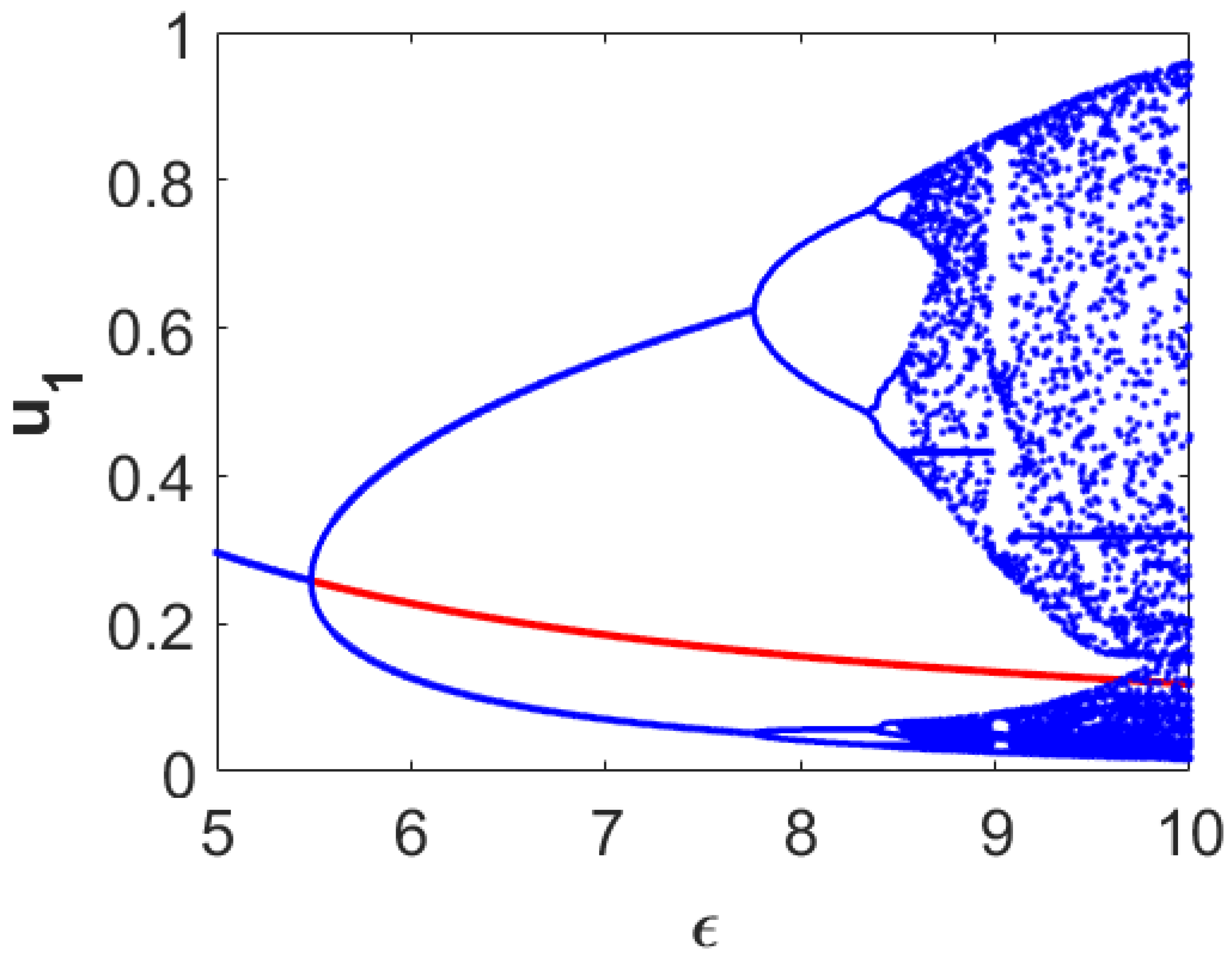
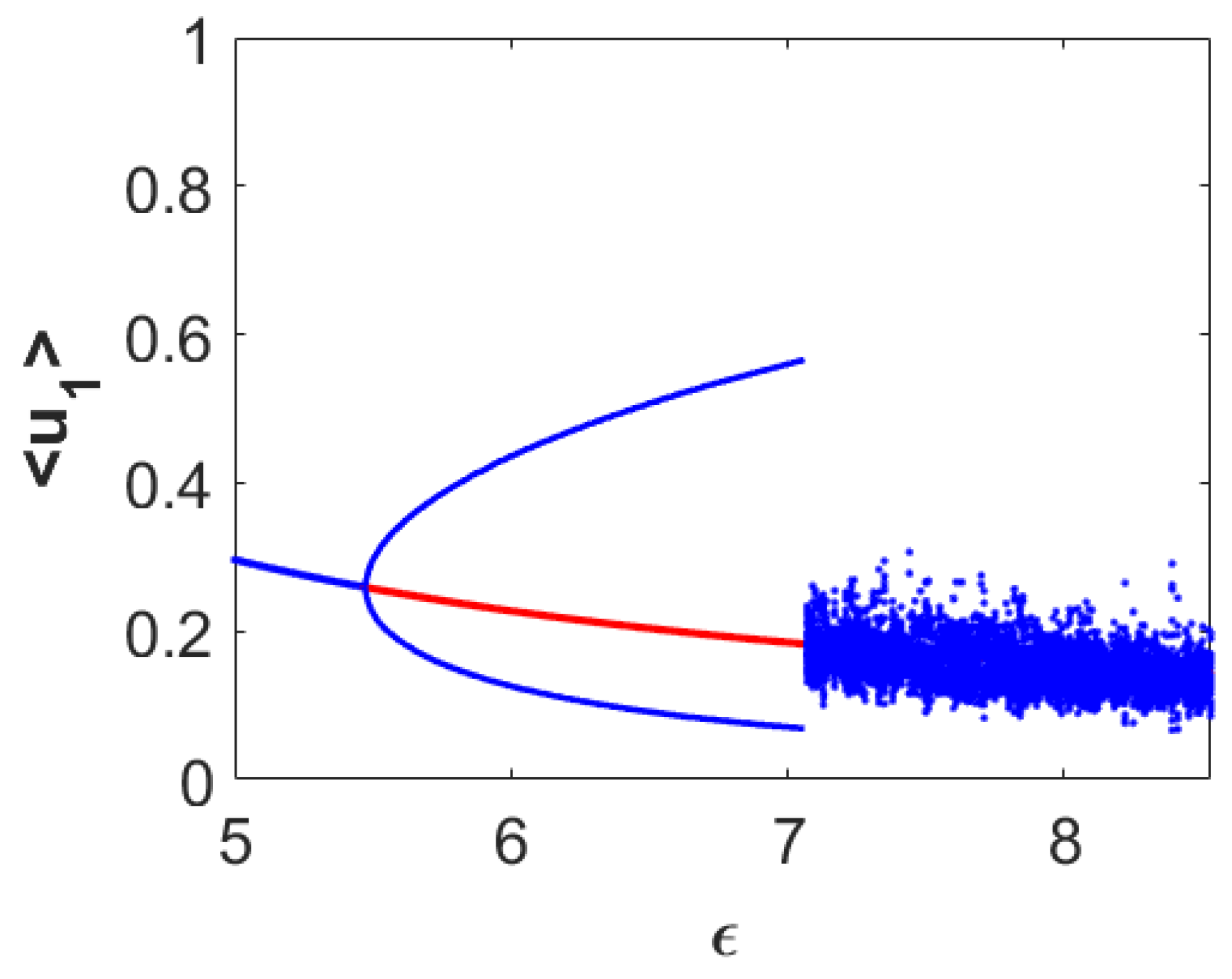
and vary the parameter $ϵ$. The resulting dynamical behaviors are encapsulated in Figure 1. From this figure, we can observe that the stable coexistence equilibrium point $E_{+++}$ loses its stability through the occurrence of Hopf bifurcation approximately at $ϵ=5.486$ and stable limit cycles appear for higher $ϵ$-values than this threshold value. The size of the limit cycle gradually increases as the $ϵ$-value moves away in positive direction from this threshold. For sufficiently large values of $ϵ$ (for example, $ϵ=8.0$), the system admits two-periodic solutions. Further increments in the value of $ϵ$ result in chaotic dynamics (for example, $ϵ=10.0$). This figure also clearly illustrates that the system takes the period-doubling route to reach chaos finally.

3. Spatiotemporal Model

In this section, we extend the temporal model (1)–(3) presented in the preceding section by incorporating the random dispersal of all the three species. The corresponding spatiotemporal model is given by

$$\begin{array}{ccc}\hfill \frac{\partial u_1}{\partial t}& =& d_1\frac{{\partial }^2{u}_1}{\partial x^2}+u_1\left(b_1-u_1-\alpha u_2-ϵv\right),\hfill \end{array}$$

(11)

$$\begin{array}{ccc}\hfill \frac{\partial u_2}{\partial t}& =& d_2\frac{{\partial }^2{u}_2}{\partial x^2}+u_2\left(b_2-\beta u_1-u_2-\mu v\right),\hfill \end{array}$$

(12)

$$\begin{array}{ccc}\hfill \frac{\partial v}{\partial t}& =& d_3\frac{{\partial }^{2}v}{\partial x^2}+v\left(-b_3+dϵu_1+d\mu u_2\right),\hfill \end{array}$$

(13)

subjected to non-negative initial conditions and periodic boundary conditions. Here, $u_1(x,t)$, $u_2(x,t)$ and $v(x,t)$ respectively denote the densities of the three species at spatial position x and time t. The bounded spatial domain is given by $[-L,L]$, where $L(>0)\in \mathbb{R}$. The positive parameters $d_i$ $(i=1,2,3)$ represent the diffusion coefficients for two prey and one predator species, respectively. Note that the equilibrium points corresponding to the temporal model (1)–(3) also serve as the spatially homogeneous steady states for the model (11)–(13).

Turing instability occurs when the stable spatially homogeneous steady state becomes unstable due to small amplitude heterogeneous perturbations around the spatially homogeneous steady state. Introducing small amplitude spatiotemporal perturbation around the spatially homogeneous coexistence steady state $E_{+++}=(u_1^{*},u_2^{*},v^{*})$ and then linearizing we find the following Jacobian matrix:

$$\begin{array}{ccc}\hfill \mathcal{J}\left(k^2\right)& =& \left[\begin{array}{ccc}-u_1^{*}-d_1{k}^2& -\alpha u_1^{*}& -ϵu_1^{*}\\ -\beta u_2^{*}& -u_2^{*}-d_2{k}^2& -\mu u_2^{*}\\ dϵv^{*}& d\mu v^{*}& -d_3{k}^2\end{array}\right],\hfill \end{array}$$

(14)

where k represents the wavenumber. Therefore, the characteristic equation is given by

$$\begin{array}{ccc}\hfill {\lambda }^3+A\left(k^2\right){\lambda }^2+B\left(k^2\right)\lambda +C\left(k^2\right)& =& 0,\hfill \end{array}$$

(15)

where

$$\begin{array}{ccc}A\left(k^2\right)& =& (d_1+d_2+d_3)k^2+u_1^{*}+u_2^{*},\hfill \\ B\left(k^2\right)& =& (d_1{d}_2+d_2{d}_3+d_3{d}_1)k^4+\{d_1{u}_2^{*}+d_2{u}_1^{*}+d_3(u_1^{*}+u_2^{*})\}{k}^2+(1-\alpha \beta )u_1^{*}{u}_2^{*}+d({ϵ}^2{u}_1^{*}+{\mu }^2{u}_2^{*})v^{*},\hfill \\ C\left(k^2\right)& =& d_1{d}_2{d}_3{k}^6+d_3(d_1{u}_2^{*}+d_2{u}_1^{*})k^4+\{d_{1}d{\mu }^2{u}_2^{*}{v}^{*}+d_{2}d{ϵ}^2{u}_1^{*}{v}^{*}+d_3(1-\alpha \beta )u_1^{*}{u}_2^{*}\}{k}^2+\{d({ϵ}^2+{\mu }^2)\hfill \\ & & -d(\alpha +\beta )ϵ\mu \}{u}_1^{*}{u}_2^{*}{v}^{*}.\hfill \end{array}$$

Now, Re($\lambda$) is less than zero provided the Routh–Hurwitz criteria are satisfied:

$$\begin{array}{c}\hfill A\left(k^2\right)>0,C\left(k^2\right)>0,A\left(k^2\right)B\left(k^2\right)-C\left(k^2\right)>0.\end{array}$$

(16)

When all the conditions presented in (16) are satisfied, then the spatially homogeneous steady state is stable. Diffusion-driven instability occurs only when one eigenvalue is zero while other two eigenvalues still have negative real parts [21,57]. If ${\lambda }_1$, ${\lambda }_2$ and ${\lambda }_3$ denote the roots of the characteristic Equation (15), then from the properties of the roots of a cubic equation we have the following relations:

$$\begin{array}{ccc}\hfill {\lambda }_1+{\lambda }_2+{\lambda }_3& =& -A\left(k^2\right),\hfill \end{array}$$

(17)

$$\begin{array}{ccc}\hfill {\lambda }_1{\lambda }_2+{\lambda }_2{\lambda }_3+{\lambda }_3{\lambda }_1& =& B\left(k^2\right),\hfill \end{array}$$

(18)

$$\begin{array}{ccc}\hfill {\lambda }_1{\lambda }_2{\lambda }_3& =& -C\left(k^2\right),\hfill \end{array}$$

(19)

$$\begin{array}{ccc}\hfill -({\lambda }_1+{\lambda }_2)({\lambda }_2+{\lambda }_3)({\lambda }_3+{\lambda }_1)& =& A\left(k^2\right)B\left(k^2\right)-C\left(k^2\right).\hfill \end{array}$$

(20)

Below the Turing bifurcation threshold, the spatially homogeneous steady state is stable and accordingly all the eigenvalues have negative real parts. At the Turing bifurcation threshold, exactly one eigenvalue becomes zero at the critical wavenumber $k_T$, whereas other two eigenvalues still have negative real parts [58]. Since at the critical wavenumber $k=k_T$ we have one of the roots is equal to zero, without any loss of generality we assume

$$\begin{array}{c}\hfill {\lambda }_1{\mid }_{k^2=k_T^2}=0,\mathrm{Re}\left({\lambda }_2\right){\mid }_{k^2=k_T^2}<0\mathrm{and}\mathrm{Re}\left({\lambda }_3\right){\mid }_{k^2=k_T^2}<0.\end{array}$$

(21)

Hence, at the critical wavenumber $k=k_T$ we obtain $C\left(k_T^2\right)=0$. Further due to the above conditions (21) for Turing instability, we get $A\left(k_T^2\right)>0$, $B\left(k_T^2\right)>0$ and $A\left(k_T^2\right)B\left(k_T^2\right)-C\left(k_T^2\right)=A\left(k_T^2\right)B\left(k_T^2\right)>0$. Thus, the system remains stable if $C\left(k^2\right)>0$ holds for all k and it becomes Turing unstable if $C\left(k^2\right)<0$ holds for at least one k. Also, $C\left(k^2\right)<0$ holds for a range of k-values around $k_T$ beyond the Turing bifurcation threshold. The expression of $C\left(k^2\right)$ can be rewritten as

$$\begin{array}{ccc}\hfill C\left(k^2\right)& \equiv & C_3{\left(k^2\right)}^3+C_2{\left(k^2\right)}^2+C_1\left(k^2\right)+C_0,\hfill \end{array}$$

(22)

where $C_3>0$ since the diffusion coefficients are positive constants and $C_0>0$ from the local asymptotic stability condition of $E_{+++}$. Also, the coefficient $C_2>0$ as the expression of it is given by $C_2=d_3(d_1{u}_2^{*}+d_2{u}_1^{*})$. The minimum for $C\left(k^2\right)$ occurs at $k=k_T$ where

$$\begin{array}{ccc}\hfill k_T^2& =& \frac{-C_2+\sqrt{C_2^2-3C_1{C}_3}}{3C_3},\hfill \end{array}$$

(23)

as we have $\frac{dC\left(k^2\right)}{d\left(k^2\right)}=0$ and $\frac{d^{2}C\left(k^2\right)}{d{\left(k^2\right)}^2}>0$ at $k=k_T$. Now from the expression (23), we can notice that $k_T^2$ is positive if $C_1<0$ or $C_2<0$ and $C_2^2>3C_1{C}_3$. Since $C_2>0$ holds for our considered system, then the condition for the positivity of $k_T^2$ reduces to $C_1<0$. Therefore, the Turing bifurcation boundary is given by

$$\begin{array}{ccc}\hfill 2C_2^3-9C_1{C}_2{C}_3-2{(C_2^2-3C_1{C}_3)}^{\frac{3}{2}}+27C_0{C}_3^2& =& 0.\hfill \end{array}$$

(24)

This is an implicit expression for the Turing bifurcation curve whenever other relevant conditions are satisfied.

Numerical Results

In this subsection, we present some numerical results in order to validate the analytical predictions and to manifest the spatiotemporal dynamics which are beyond the scope of linear analysis. For this purpose, we considered a set of parameter values

$$\begin{array}{c}\hfill b_1=1.0,\alpha =1.0,b_2=1.0,\beta =1.5,\mu =1.0,d=0.5,b_3=1.0,d_1=0.1,d_2=0.2,\end{array}$$

(25)

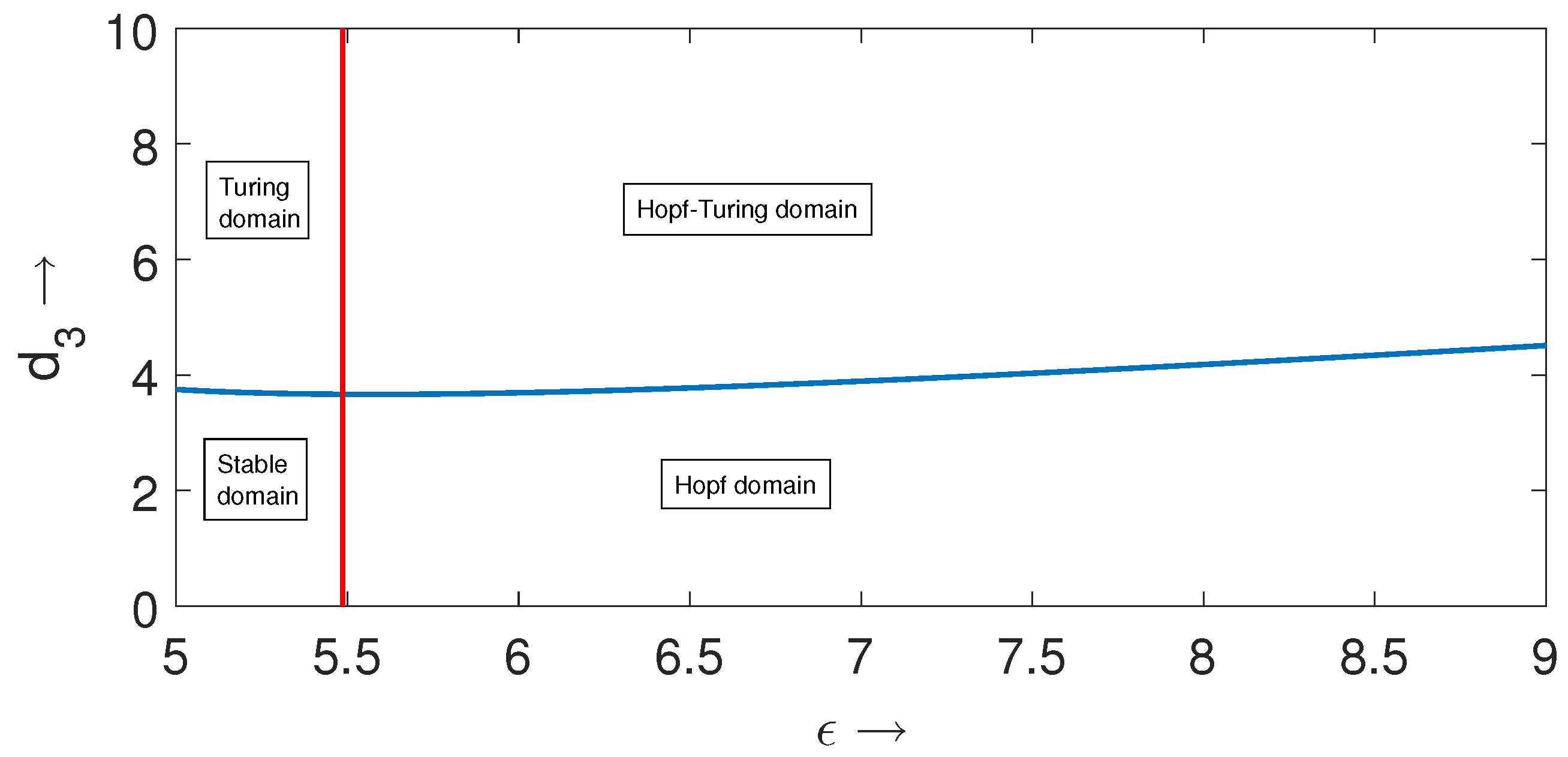
and varied the parameters $ϵ$ and $d_3$. For this set of parameter values, the temporal-Hopf bifurcation threshold is approximately given by $ϵ=5.486$. First, we present the temporal-Hopf and Turing bifurcation curves for the local spatiotemporal model (11)–(13) in $(ϵ,d_3)$-parameter space in Figure 2. From this figure, we can notice that these two bifurcation curves divide the two-dimensional parameter space into four different regions, such as stable region (left to the temporal-Hopf curve and below the Turing curve), Turing region (left to the temporal-Hopf curve and above the Turing curve), Hopf–Turing region (right to the temporal-Hopf curve and above the Turing curve) and pure Hopf region (right to the temporal-Hopf curve and below the Turing curve).

Before proceeding further, here we briefly describe about the numerical discretization of the system (11)–(13). We have used the forward Euler scheme and central difference scheme to discretize the reaction and diffusion parts, respectively. The periodic boundary conditions have been employed at the boundary of the computational domain. For all the patterns presented in this subsection, we have used the following pulse-type initial conditions:

$$\begin{array}{ccc}\hfill u_1(x,0)& =& \left\{\begin{array}{cc}{u}_1^{*}+{\eta }_1,\hfill & |x|<10,\hfill \\ u_1^{*},\hfill & 10\le |x|\le L,\hfill \end{array}\right.\hfill \\ \hfill u_2(x,0)& =& \left\{\begin{array}{cc}{u}_2^{*}+{\eta }_2,\hfill & |x|<10,\hfill \\ u_2^{*},\hfill & 10\le |x|\le L,\hfill \end{array}\right.\hfill \\ \hfill v(x,0)& =& \left\{\begin{array}{cc}{v}^{*}+{\eta }_3,\hfill & |x|<10,\hfill \\ v^{*},\hfill & 10\le |x|\le L,\hfill \end{array}\right.\hfill \end{array}$$

(26)

where $|{\eta }_r|\ll 1$, for $r=1,2,3$.

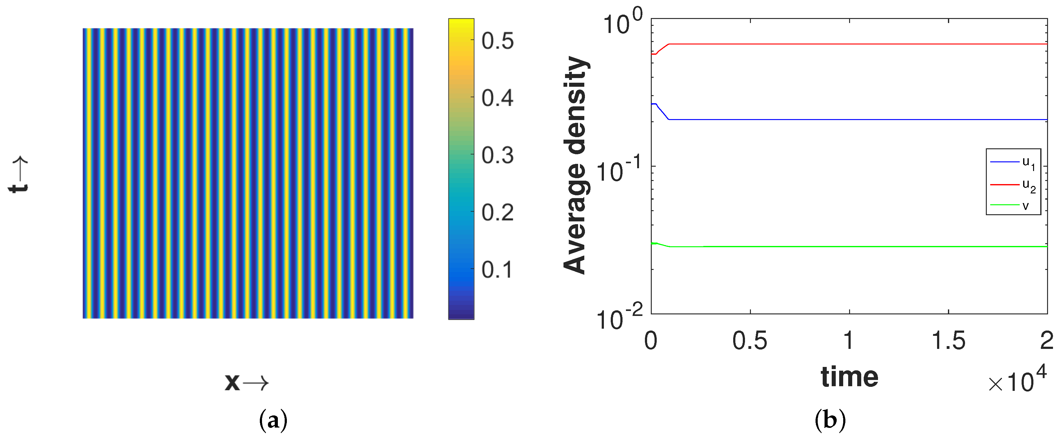
Now, we consider a point $(ϵ,d_3)=(5.4,9.0)$, which lies in the Turing region. For this choice of $ϵ$, we obtain the coexistence steady state $E_{+++}=(0.2641,0.5738,0.03)$ which is locally asymptotically stable in the absence of diffusion. Figure 3 shows the stationary Turing pattern produced by $u_1$-component and the corresponding temporal evolution of the average densities of all considered species. 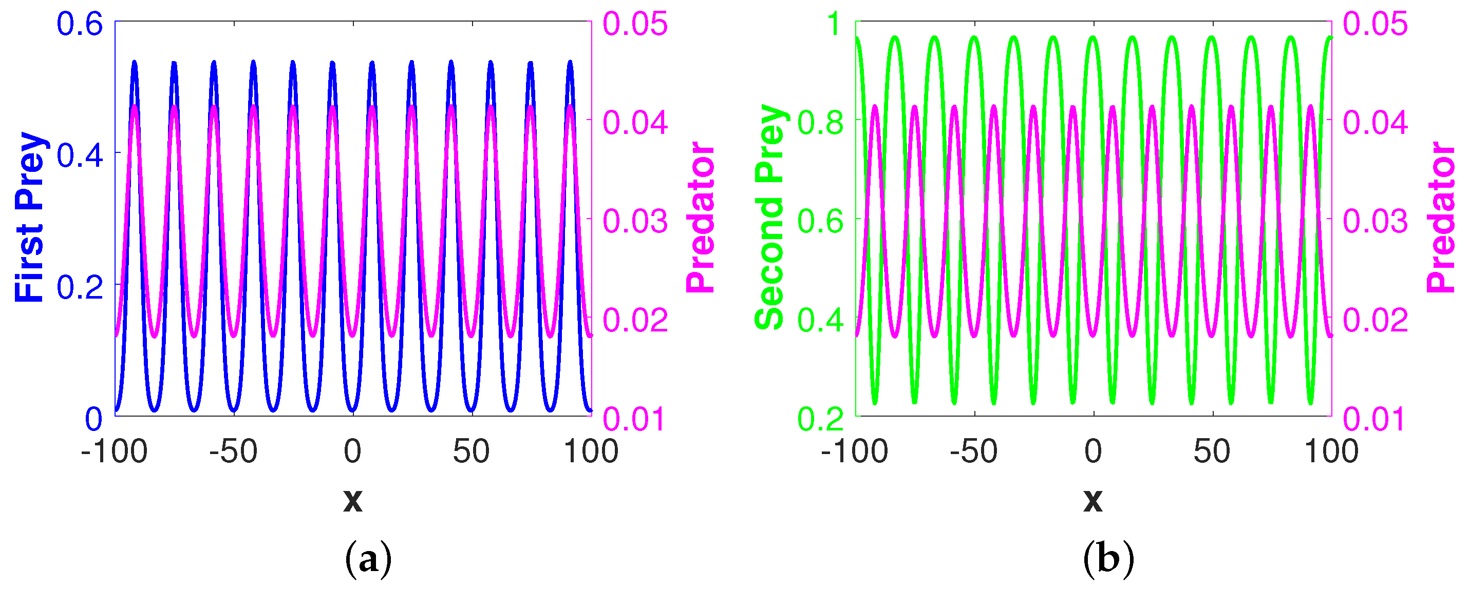We would like to mention here that the patterns for the second prey and predator species are qualitatively similar with the pattern for the first prey species presented in Figure 3a. However, the regions with high first prey density correspond to the same for predator but to low second prey density. These scenarios for the density correlation among the three considered species are presented in Figure 4. This type of density correlation among the three considered species has also been observed for other patterns presented in this section. Also, note that we have considered the one-dimensional spatial domain $[-100,100]$ for the clarity of understanding in Figure 4, but all the patterns presented in this section are obtained for the spatial domain $[-200,200]$.

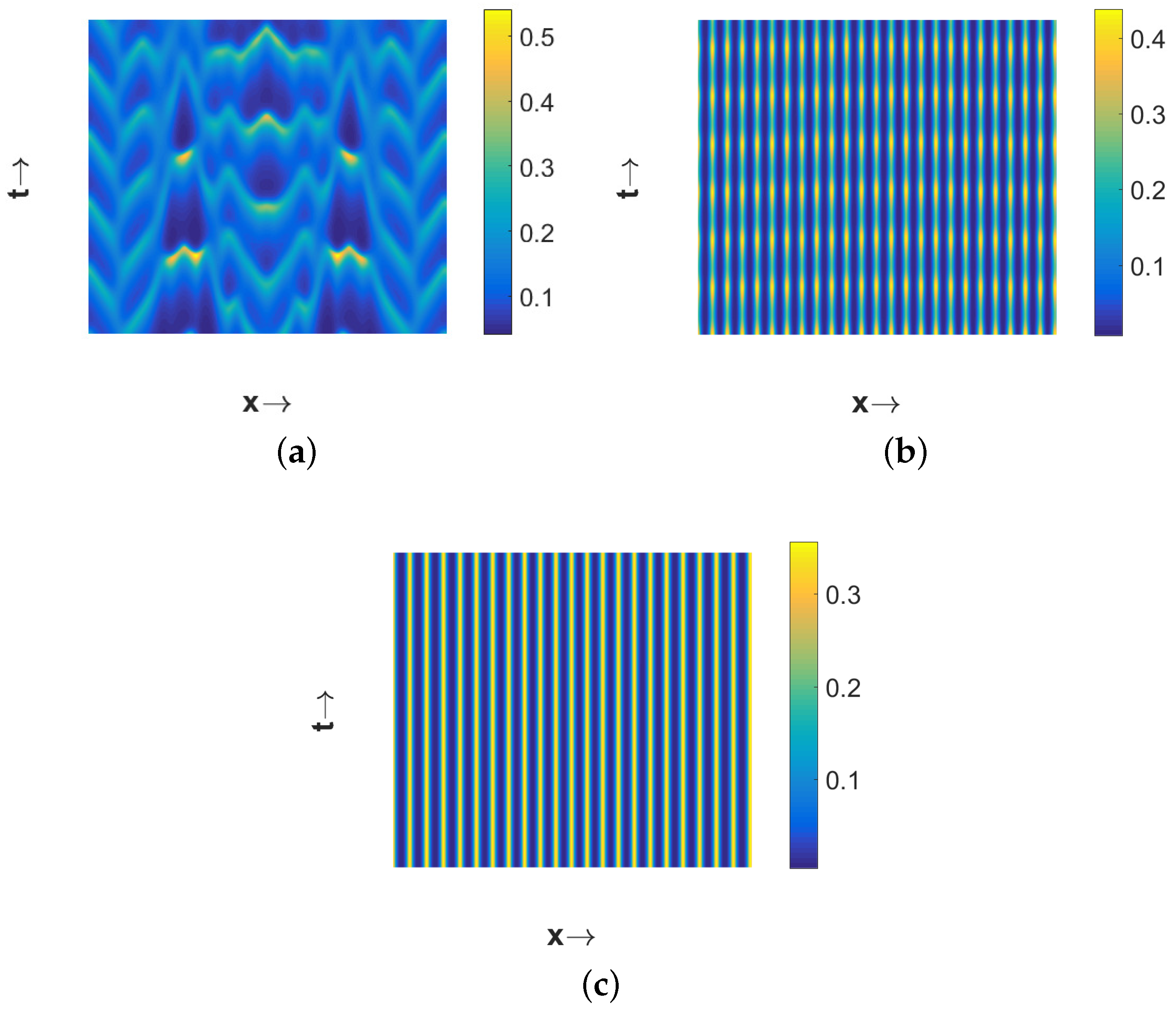
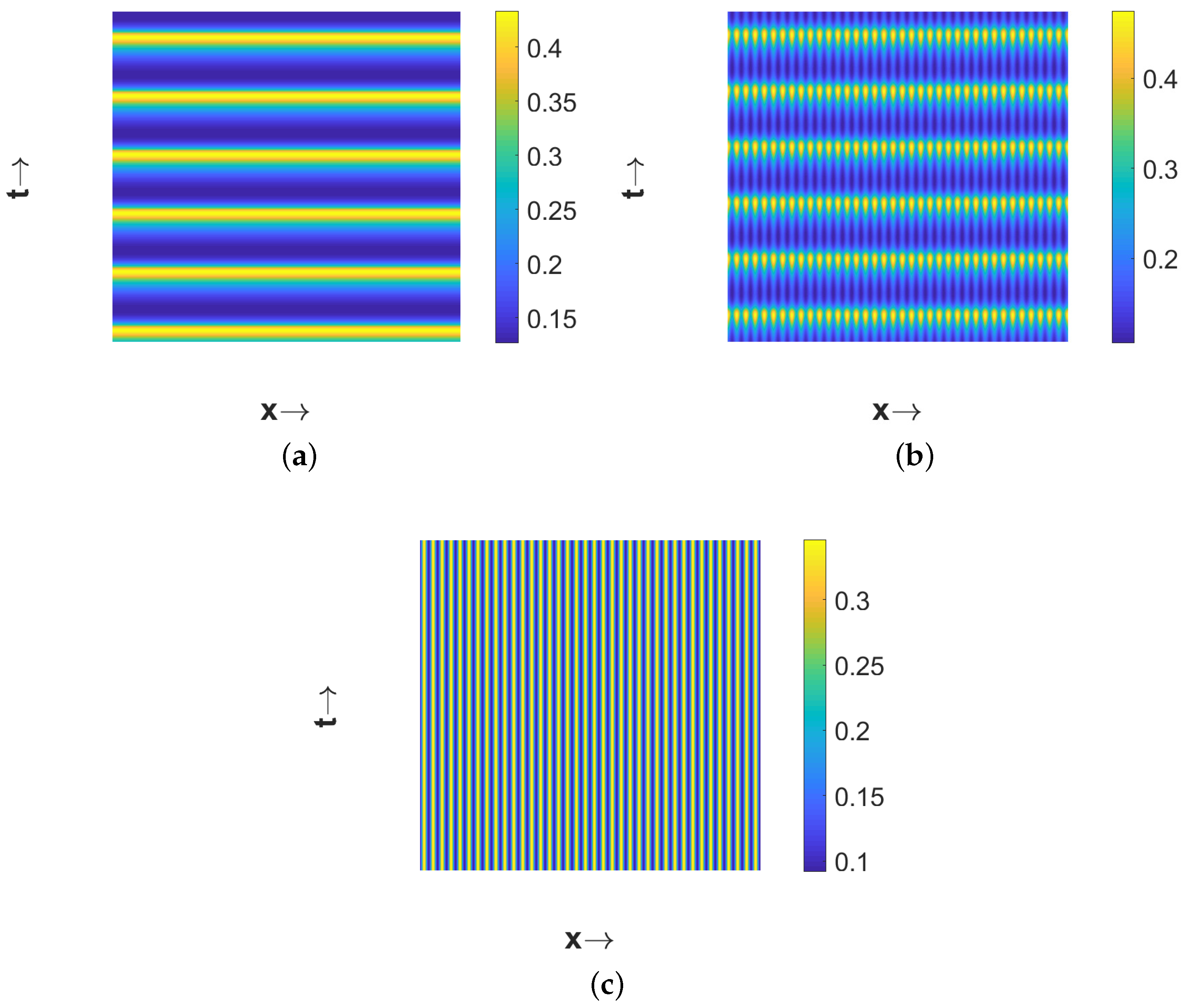
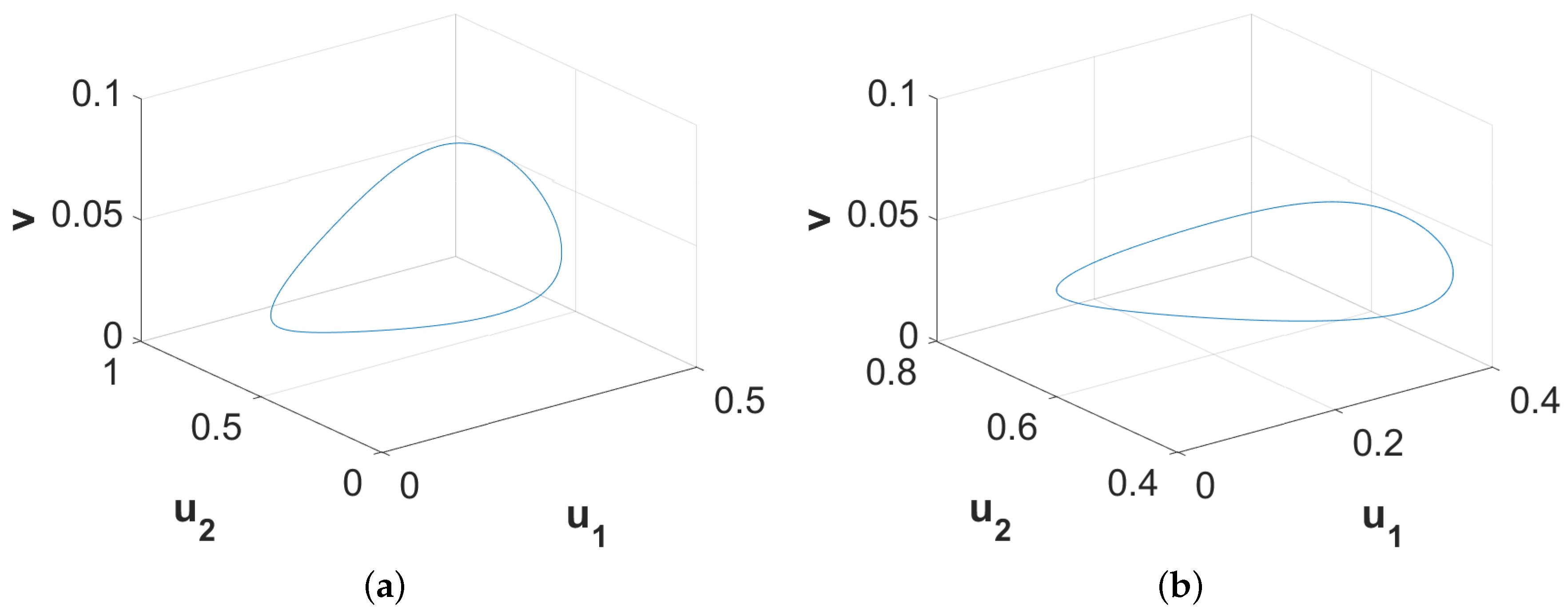
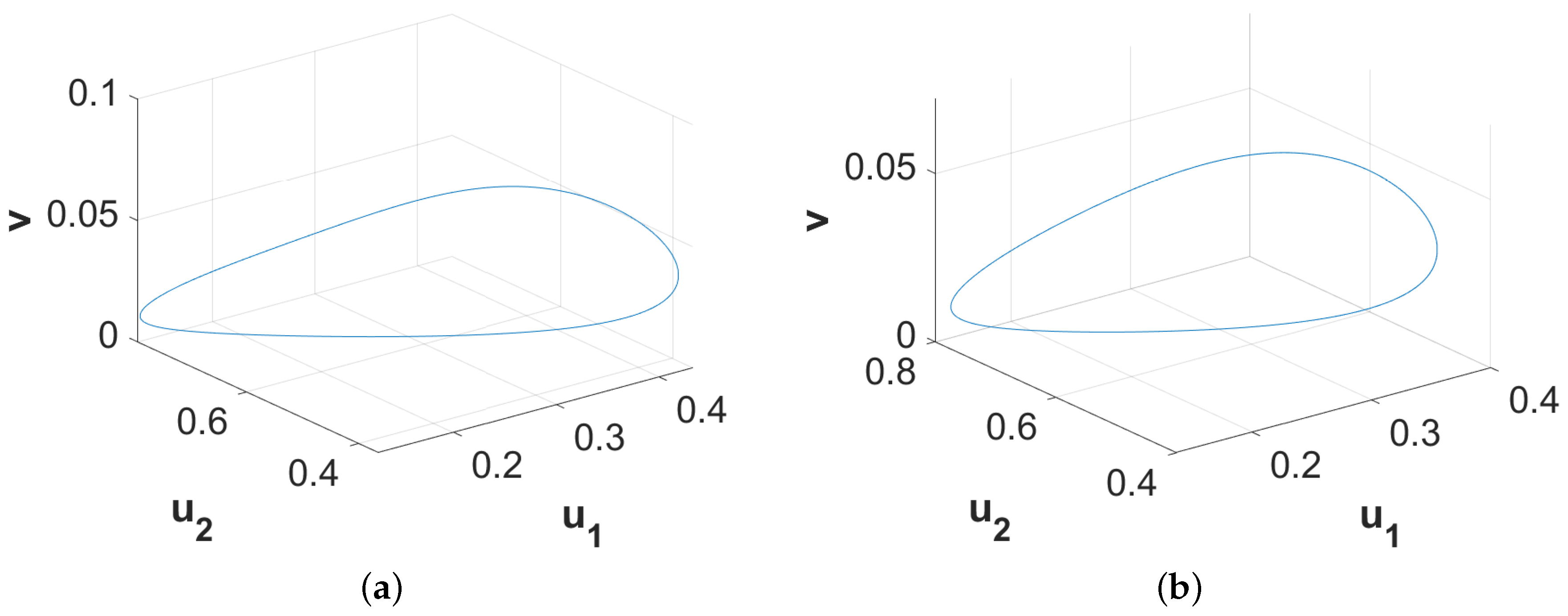
Now if we choose $ϵ=6.0$, then $E_{+++}=(0.2273,0.6364,0.0227)$ is unstable, due to temporal-Hopf bifurcation, in the absence of diffusion terms. Hence, we can observe homogeneous in space and periodic in time pattern for $d_3=3.0$ in Figure 5a, periodic in both space and time pattern for $d_3=3.75$ in Figure 5b, and periodic in space but stationary in time pattern for $d_3=9.0$ in Figure 5c. Phase diagrams presented in Figure 6 confirm the temporal periodicity of the patterns presented in Figure 5a,b, respectively. In Figure 7, we present the bifurcation diagram for spatially averaged density of first prey species in order to illustrate the transition of different types of patterns depending on the value of the diffusion coefficient $d_3$ for $ϵ=6.0$. In order to prepare this bifurcation diagram, we have used small pulse type perturbation about the mid-point around the spatially homogeneous steady state for each $d_3$-value and then plotted the maxima and minima of spatially averaged densities. From this figure, we can observe that periodic in time and homogeneous in space pattern persists up to $d_3=3.67$. The periodic in both space and time pattern exists for $d_3\in [3.68,3.91]$ and then stationary pattern emerges for $d_3>3.91$. Interestingly, the number of patches with high first prey density gradually decreases with the increment in the value of $d_3$.

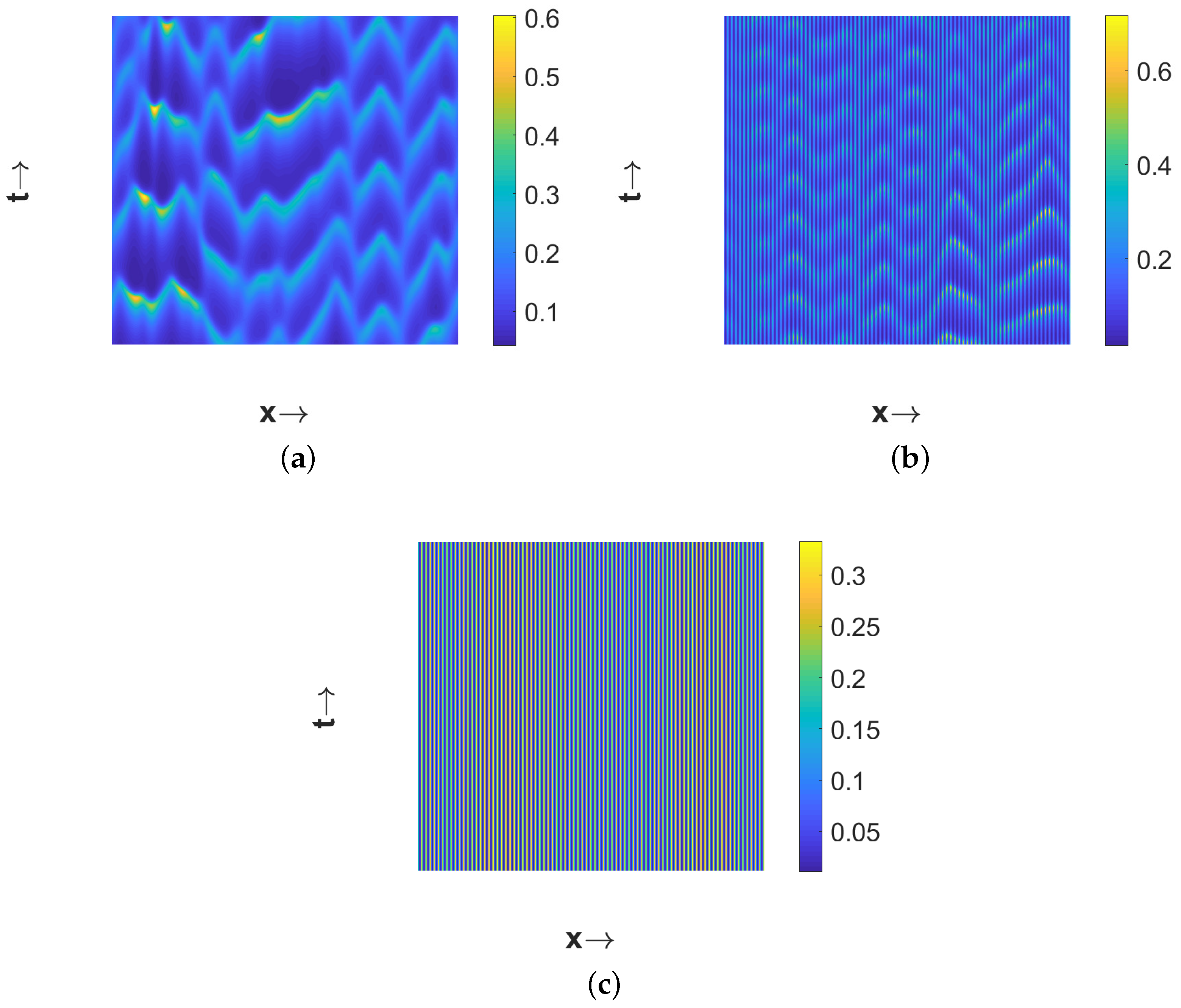
If we further increase the magnitude of $ϵ$ to $8.0$, then the system (11)–(13) admits the spatially homogeneous coexistence steady state $E_{+++}=(0.1556,0.7556,0.0111)$ which is temporally unstable. Then the choice $d_3=1.0$ leads to the spatiotemporal chaotic pattern (see Figure 8a). A close look at the chaotic pattern reveals that the distribution of the species is symmetric about the midpoint in space and this is due to our consideration of the symmetric pulse type initial conditions. The chaotic nature has been cross verified by checking the sensitivity to initial conditions as described in [59], but we do not present the results here for the sake of brevity. Interestingly, spatiotemporal chaotic pattern disappears and eventually settles to a stationary pattern for a higher value of $d_3$ (for example, $d_3=10.0$). This transition from spatiotemporal chaotic to stationary pattern takes place via a pattern where patches move periodically for intermediate values of $d_3$ (for example, $d_3=9.5$). 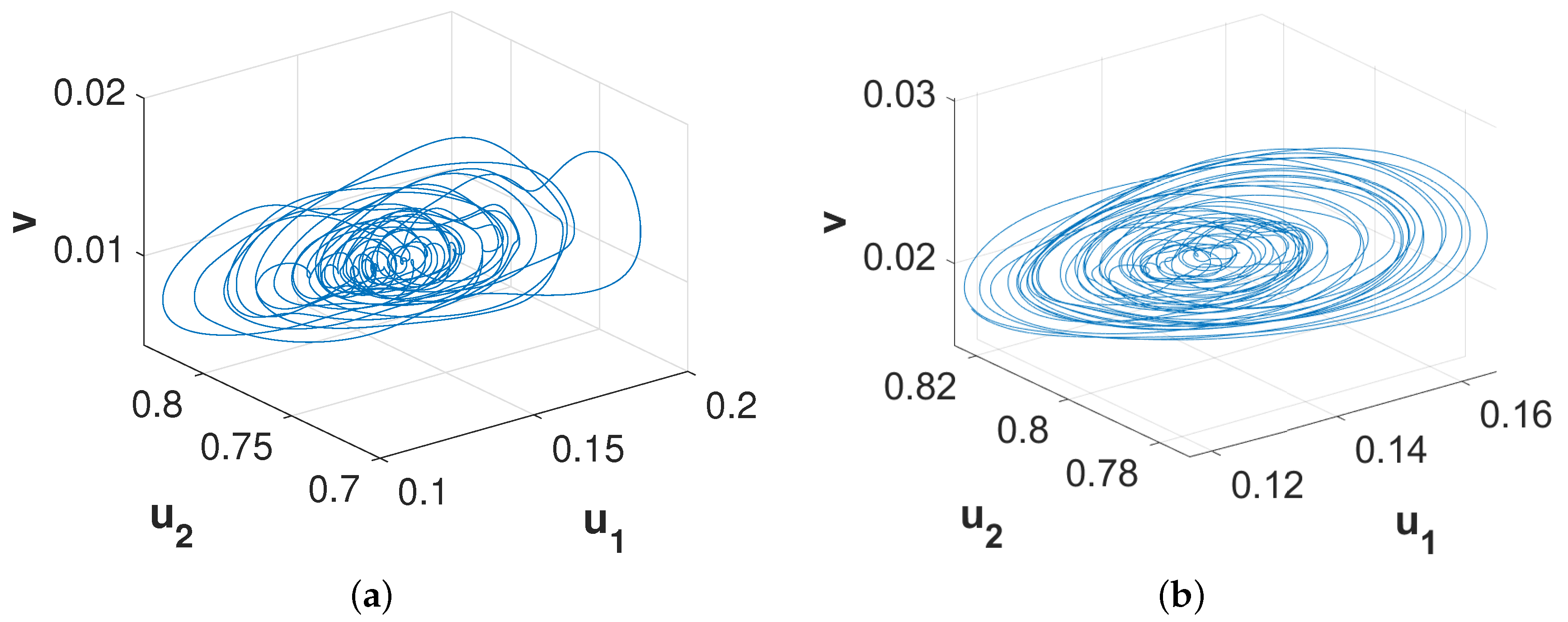The resulting patterns are presented in Figure 8. The phase diagrams presented in Figure 9 confirm the chaotic nature of the pattern presented in Figure 8a and the periodic nature of the pattern presented in Figure 8b.

All patterns exhibited in Figure 3a, Figure 5 and Figure 8 are stable in the sense that their nature will not alter with further increment in time. However, the considered system (11)–(13) can produce long transient patterns in order to reach the final stable patterns. Such an instance of long transient pattern can be found for $ϵ=8.0$ and $d_3=9.0$ along with other parameter values mentioned above. 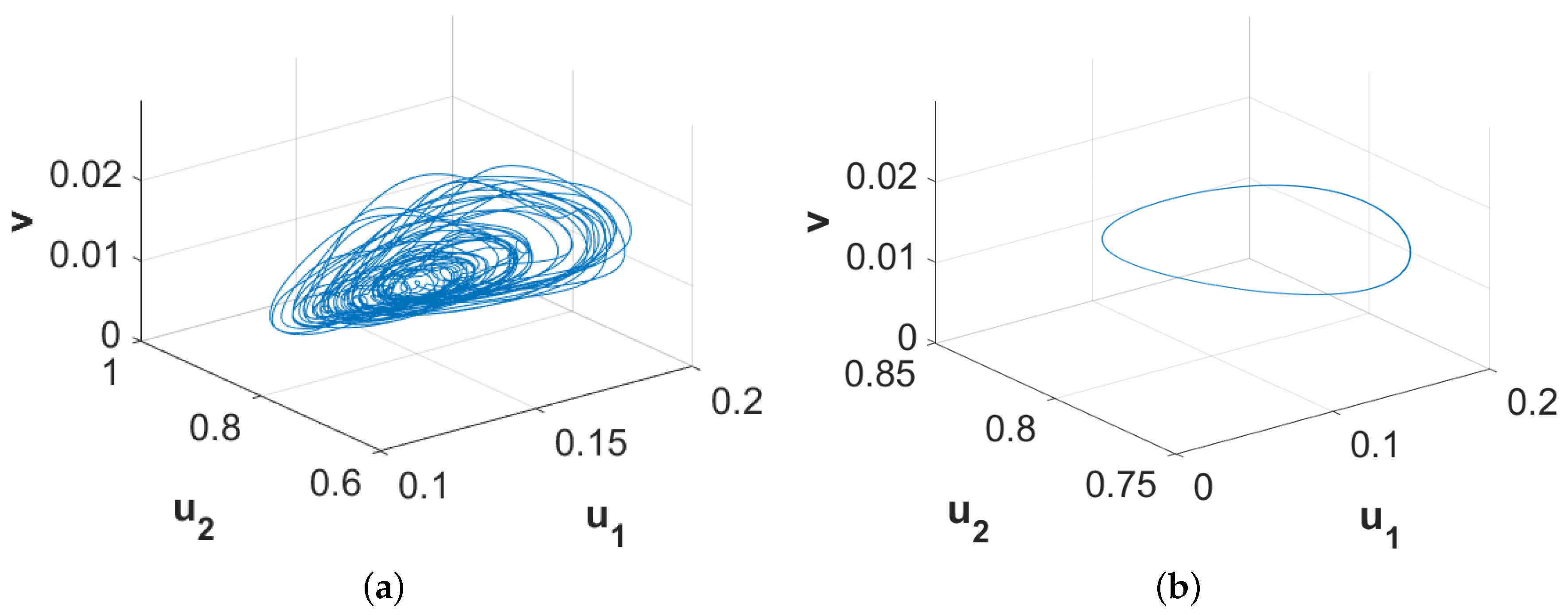Figure 10 exhibits the phase diagrams for the spatially averaged densities of the considered three species for $t\in [18,000,20,000]$ and $t\in [58,000,60,000]$, respectively. Since the phase diagram presented in Figure 10a is restricted to an annular region, we can term the nature of the corresponding spatiotemporal distribution as quasi-periodic which persists for approximately $t=50,000$. On the other hand, the phase diagram presented in Figure 10b clearly shows the periodic nature of the corresponding spatiotemporal distribution and this pattern is stable for the considered parameter values. With the increment in time, the width of the annular region gradually decreases and finally the region settles into a limit cycle. However, this long time period for the existence of quasi-stable and quasi-periodic pattern can be few or even hundreds of generations for certain species. Therefore, this type of existence of long transient pattern and then finally convergence into a stable pattern can provide an alternative explanation for ecological regime shifts apart from the usual concept of exogenously sparked regime shifts.

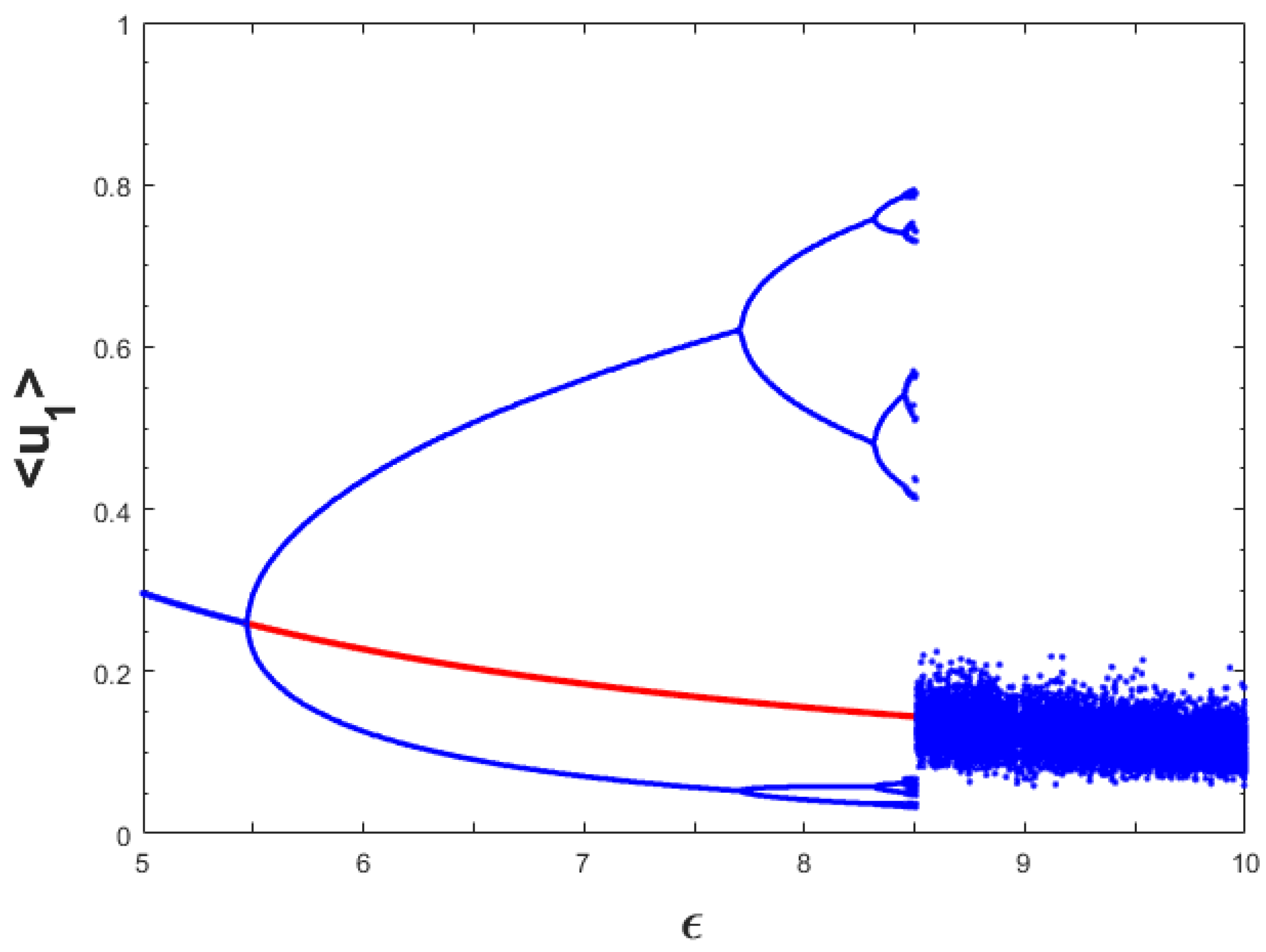
Now, we want to investigate the influence of random dispersal of the three species on the dynamics presented in Figure 1 for the temporal model. For this purpose, we considered the same parameter values as for Figure 1 with $d_1=0.1$, $d_2=0.2$ and $d_3=1.0$, and varied the value of the parameter $ϵ$. By employing spatially homogeneous initial population distributions slightly perturbed from the spatially homogeneous coexistence steady state, we found the bifurcation diagram which was more or less similar to the Figure 1 and chose not to display it here for the sake of brevity. However, consideration of pulse type initial population distributions led to different dynamical behaviors for a certain range of $ϵ$-values and the resulting dynamics are encapsulated in Figure 11. Comparing Figure 1 and Figure 11, we can observe that the dynamics for both the models were same up to $ϵ=8.5$ approximately. For higher values of $ϵ$ (that is, $ϵ\in (8.5,10.0]$), we observed the difference in chaotic dynamics. For spatiotemporal model (11)–(13), the amplitudes of chaotic oscillations were much less than that of the temporal case. We can attribute the reason for this type of phenomenon to the emergence of spatial heterogeneity in the population distributions as we have found spatially heterogeneous chaotic distributions in this case.

Further, we examined the stability of this bifurcation diagram by employing both the forward and backward continuation techniques. In order to construct a bifurcation diagram using forward continuation technique, we employed the following algorithm:

• First, consider a pulse-type initial condition for the starting value of the bifurcation parameter and run the simulation for sufficient time period such that a stable state is reached.
• Make a tiny increment in the value of the bifurcation parameter.
• Then, use the stable state obtained in the previous step as an initial condition for the present value of the bifurcation parameter and run the simulation till a stable state is reached.
• Continue the previous two steps till the last value of the bifurcation parameter is reached.

In a similar manner, one can efficiently construct a bifurcation diagram using backward continuation technique by reversing the process encapsulated in the above algorithm. Forward continuation technique results in more or less similar bifurcation diagram as the Figure 11 and accordingly we do not include it here. On the other hand, we observed significant changes in the bifurcation diagram using backward continuation technique and the resulting dynamics are encapsulated in Figure 12. From this diagram, we can observe that the period-doubling route to chaos has been destroyed and spatially heterogeneous chaotic regime survives for larger range of $ϵ$-values. Overall, bifurcation diagrams presented in Figure 1, Figure 11 and Figure 12 indicate the existence of alternative stable states for the model (11)–(13). Note that these states indicate the coexistence of all the three species and can be both the spatially homogeneous and heterogeneous population distributions.

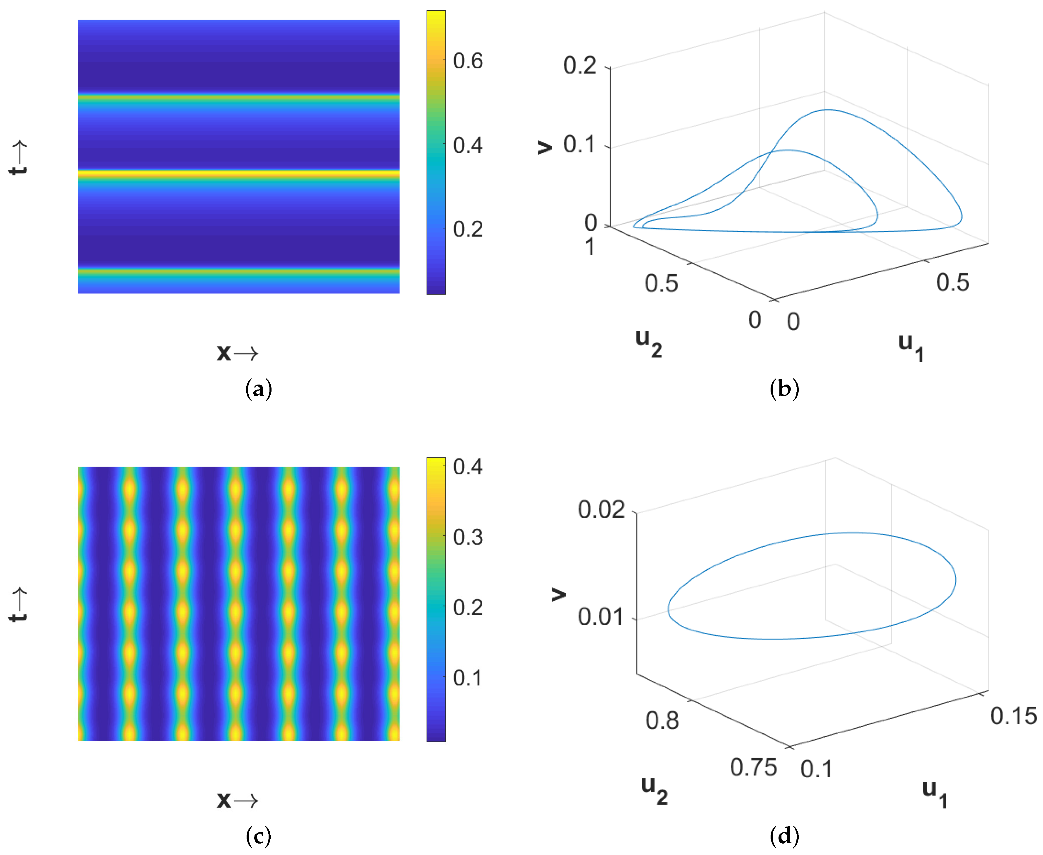
Another interesting finding is that the spatial population distributions depended on the spatial domain size when the parameter values were taken far from the temporal-Hopf bifurcation threshold. The patterns presented in Figure 13 are numerically computed over the one-dimensional spatial domain $[-50,50]$ with the same parameter values used for Figure 8a,c. Figure 13a suggests that the smaller domain size can produce a two-periodic pattern while the larger domain size produces a chaotic one. Also, Figure 13c indicates that the smaller domain size can give rise to periodic in both the space and time population distribution while the larger domain size gives a stationary heterogeneous distribution. The two-periodic and periodic nature of the patterns presented in Figure 13a,c can be confirmed by the phase portraits of the spatially averaged densities in Figure 13b,d, respectively. However, we did not find any effect of the domain size on the resulting patterns presented in Figure 3, Figure 5 and Figure 8b. Therefore, our numerical findings suggest that not only certain parameters associated with a model play crucial roles in the emergence of different types of spatial population distributions but also the spatial domain size can potentially play a key role in shaping the population distributions.

4. Nonlocal Model

In this section, we further extend the spatiotemporal model (11)–(13) by incorporating nonlocal intra-specific competition for both the prey species. Accordingly, the model (11)–(13) becomes

$$\begin{array}{ccc}\hfill \frac{\partial u_1}{\partial t}& =& d_1\frac{{\partial }^2{u}_1}{\partial x^2}+u_1\left(b_1-J\left(u_1\right)-\alpha u_2-ϵv\right),\hfill \end{array}$$

(27)

$$\begin{array}{ccc}\hfill \frac{\partial u_2}{\partial t}& =& d_2\frac{{\partial }^2{u}_2}{\partial x^2}+u_2\left(b_2-\beta u_1-J\left(u_2\right)-\mu v\right),\hfill \end{array}$$

(28)

$$\begin{array}{ccc}\hfill \frac{\partial v}{\partial t}& =& d_3\frac{{\partial }^{2}v}{\partial x^2}+v\left(-b_3+dϵu_1+d\mu u_2\right),\hfill \end{array}$$

(29)

where

$$\begin{array}{ccc}\hfill J\left(u_r\right)& =& {\int }_{-\infty }^{\infty }{u}_r(y,t){\varphi }_r(x-y)dy,r=1,2,\hfill \end{array}$$

which take care of the nonlocality in intra-specific interactions for both the prey species arising primarily as a result of nonlocal consumption of resources. However, there exist other mechanisms such as cannibalism, space sharing, fights, etc., which can eventually lead to nonlocal intra-specific competition. The nonlocal system (27)–(29) is subjected to the same initial and boundary conditions mentioned before for the local spatiotemporal system (11)–(13). Here, the functions ${\varphi }_r$ ($r=1,2$) represent the non-negative kernel functions. Further, in order to capture the unbiased movement of the two prey populations we assume the kernel functions ${\varphi }_r$ ($r=1,2$) as even functions. Throughout this paper, we restrict ourselves only to the top-hat kernel functions defined as follows:

$$\begin{array}{ccc}\hfill {\varphi }_r\left(x\right)& =& \left\{\begin{array}{c}\frac{1}{2{\delta }_r},|x|\le {\delta }_r,\hfill \\ 0,\mathrm{otherwise},\hfill \end{array}\right.\hfill \end{array}$$

(30)

for $r=1,2$. The newly introduced parameters ${\delta }_r$ ($r=1,2$) represent the extent of the nonlocality by controlling the width of the kernel functions ${\varphi }_r$. Also, one can easily verify that the spatially homogeneous steady states of the nonlocal system (27)–(29) are same as that of the corresponding local system (11)–(13) and accordingly we use the same notations for them.

In order to linearize the nonlocal system (27)–(29) about the spatially homogeneous coexistence steady state $E_{+++}=(u_1^{*},u_2^{*},v^{*})$, we introduce the perturbation $u_1=u_1^{*}+\epsilon {\tilde{u}}_1{e}^{\lambda t+ikx}$, $u_2=u_2^{*}+\epsilon {\tilde{u}}_2{e}^{\lambda t+ikx}$ and $v=v^{*}+\epsilon \tilde{v}{e}^{\lambda t+ikx}$ with $\mid \epsilon \mid \ll 1$. Then the Jacobian matrix corresponding to the linearized system is given by

$$\begin{array}{ccc}\hfill \tilde{\mathcal{J}}(k,{\delta }_1,{\delta }_2)& =& \left[\begin{array}{ccc}-u_1^{*}{\int }_{-\infty }^{\infty }{\varphi }_1\left(y\right)e^{-iky}dy-d_1{k}^2& -\alpha u_1^{*}& -ϵu_1^{*}\\ -\beta u_2^{*}& -u_2^{*}{\int }_{-\infty }^{\infty }{\varphi }_2\left(y\right)e^{-iky}dy-d_2{k}^2& -\mu u_2^{*}\\ dϵv^{*}& d\mu v^{*}& -d_3{k}^2\end{array}\right]\hfill \\ & =& \left[\begin{array}{ccc}-u_1^{*}\frac{sin\left(k{\delta }_1\right)}{k{\delta }_1}-d_1{k}^2& -\alpha u_1^{*}& -ϵu_1^{*}\\ -\beta u_2^{*}& -u_2^{*}\frac{sin\left(k{\delta }_2\right)}{k{\delta }_2}-d_2{k}^2& -\mu u_2^{*}\\ dϵv^{*}& d\mu v^{*}& -d_3{k}^2\end{array}\right].\hfill \end{array}$$

(31)

Therefore, the characteristic equation is given by

$$\begin{array}{ccc}\hfill {\lambda }^3+\tilde{A}(k,{\delta }_1,{\delta }_2){\lambda }^2+\tilde{B}(k,{\delta }_1,{\delta }_2)\lambda +\tilde{C}(k,{\delta }_1,{\delta }_2)& =& 0,\hfill \end{array}$$

(32)

where

$$\begin{array}{ccc}\hfill \tilde{A}(k,{\delta }_1,{\delta }_2)& =& (d_1+d_2+d_3)k^2+u_1^{*}\frac{sin\left(k{\delta }_1\right)}{k{\delta }_1}+u_2^{*}\frac{sin\left(k{\delta }_2\right)}{k{\delta }_2},\hfill \end{array}$$

(33)

$$\begin{array}{ccc}\hfill \tilde{B}(k,{\delta }_1,{\delta }_2)& =& d_3{k}^2\left\{(d_1+d_2)k^2+u_1^{*}\frac{sin\left(k{\delta }_1\right)}{k{\delta }_1}+u_2^{*}\frac{sin\left(k{\delta }_2\right)}{k{\delta }_2}\right\}+\left(d_1{k}^2+u_1^{*}\frac{sin\left(k{\delta }_1\right)}{k{\delta }_1}\right)\left(d_2{k}^2+u_2^{*}\frac{sin\left(k{\delta }_2\right)}{k{\delta }_2}\right)\hfill \\ & & +d({ϵ}^2{u}_1^{*}+{\mu }^2{u}_2^{*})v^{*}-\alpha \beta u_1^{*}{u}_2^{*}\hfill \\ & =& (d_1{d}_2+d_2{d}_3+d_3{d}_1)k^4+\left\{d_1{u}_2^{*}\frac{sin\left(k{\delta }_2\right)}{k{\delta }_2}+d_2{u}_1^{*}\frac{sin\left(k{\delta }_1\right)}{k{\delta }_1}+d_3\left(u_1^{*}\frac{sin\left(k{\delta }_1\right)}{k{\delta }_1}+u_2^{*}\frac{sin\left(k{\delta }_2\right)}{k{\delta }_2}\right)\right\}{k}^2\hfill \\ & & +\left(\frac{sin\left(k{\delta }_1\right)sin\left(k{\delta }_2\right)}{k^2{\delta }_1{\delta }_2}-\alpha \beta \right)u_1^{*}{u}_2^{*}+d({ϵ}^2{u}_1^{*}+{\mu }^2{u}_2^{*})v^{*},\hfill \end{array}$$

(34)

$$\begin{array}{ccc}\hfill \tilde{C}(k,{\delta }_1,{\delta }_2)& =& d_3{k}^2\left(d_1{k}^2+u_1^{*}\frac{sin\left(k{\delta }_1\right)}{k{\delta }_1}\right)\left(d_2{k}^2+u_2^{*}\frac{sin\left(k{\delta }_2\right)}{k{\delta }_2}\right)+d{ϵ}^2{u}_1^{*}{v}^{*}\left(d_2{k}^2+u_2^{*}\frac{sin\left(k{\delta }_2\right)}{k{\delta }_2}\right)+\hfill \\ & & d{\mu }^2{u}_2^{*}{v}^{*}\left(d_1{k}^2+u_1^{*}\frac{sin\left(k{\delta }_1\right)}{k{\delta }_1}\right)-d_3\alpha \beta u_1^{*}{u}_2^{*}{k}^2-d(\alpha +\beta )ϵ\mu u_1^{*}{u}_2^{*}{v}^{*}\hfill \\ & =& d_1{d}_2{d}_3{k}^6+d_3\left\{d_1{u}_2^{*}\frac{sin\left(k{\delta }_2\right)}{k{\delta }_2}+d_2{u}_1^{*}\frac{sin\left(k{\delta }_1\right)}{k{\delta }_1}\right\}{k}^4+\hfill \\ & & \left\{d_{1}d{\mu }^2{u}_2^{*}{v}^{*}+d_{2}d{ϵ}^2{u}_1^{*}{v}^{*}+d_3\left(\frac{sin\left(k{\delta }_1\right)sin\left(k{\delta }_2\right)}{k^2{\delta }_1{\delta }_2}-\alpha \beta \right)u_1^{*}{u}_2^{*}\right\}{k}^2\hfill \\ & & +d\left\{\left({ϵ}^2\frac{sin\left(k{\delta }_2\right)}{k{\delta }_2}+{\mu }^2\frac{sin\left(k{\delta }_1\right)}{k{\delta }_1}\right)-(\alpha +\beta )ϵ\mu \right\}{u}_1^{*}{u}_2^{*}{v}^{*}.\hfill \end{array}$$

(35)

Using the Routh–Hurwitz criteria, we can say that the spatially homogeneous coexistence steady state $E_{+++}=(u_1^{*},u_2^{*},v^{*})$ will be asymptotically stable if and only if

$$\begin{array}{c}\hfill \tilde{A}(k,{\delta }_1,{\delta }_2)>0,\tilde{C}(k,{\delta }_1,{\delta }_2)>0,\tilde{A}(k,{\delta }_1,{\delta }_2)\tilde{B}(k,{\delta }_1,{\delta }_2)-\tilde{C}(k,{\delta }_1,{\delta }_2)>0.\end{array}$$

(36)

In order to attain Turing instability threshold we need to have one zero eigenvalue and other two eigenvalues with negative real parts. Following the process described in the previous section, the conditions for achieving Turing instability threshold imply the following conditions:

$$\begin{array}{c}\hfill \tilde{A}(k,{\delta }_1,{\delta }_2)>0,\tilde{B}(k,{\delta }_1,{\delta }_2)>0,\tilde{C}(k,{\delta }_1,{\delta }_2)=0.\end{array}$$

(37)

Note that the expressions of $\tilde{A}$, $\tilde{B}$ and $\tilde{C}$ are transcendental in nature of their arguments k, ${\delta }_1$ and ${\delta }_2$. The associated Turing bifurcation threshold can be obtained by solving the following two equations simultaneously

$$\begin{array}{c}\hfill \tilde{C}(k,{\delta }_1,{\delta }_2)=0,\frac{\partial }{\partial k}\tilde{C}(k,{\delta }_1,{\delta }_2)=0.\end{array}$$

(38)

Solving the first equation of (38) for $d_3$, we obtain

$$\begin{array}{ccc}\hfill d_3& =& -\frac{d\left\{(d_1{\mu }^2{u}_2^{*}+d_2{ϵ}^2{u}_1^{*})k^2+\left({ϵ}^2\frac{sin\left(k{\delta }_2\right)}{k{\delta }_2}+{\mu }^2\frac{sin\left(k{\delta }_1\right)}{k{\delta }_1}-(\alpha +\beta )ϵ\mu \right)u_1^{*}{u}_2^{*}\right\}{v}^{*}}{d_1{d}_2{k}^6+\left\{d_1{u}_2^{*}\frac{sin\left(k{\delta }_2\right)}{{\delta }_2}+d_2{u}_1^{*}\frac{sin\left(k{\delta }_1\right)}{{\delta }_1}\right\}{k}^3+\left\{\frac{sin\left(k{\delta }_1\right)sin\left(k{\delta }_2\right)}{k^2{\delta }_1{\delta }_2}-\alpha \beta \right\}{u}_1^{*}{u}_2^{*}{k}^2}.\hfill \end{array}$$

(39)

Now, differentiating $\tilde{C}(k,{\delta }_1,{\delta }_2)$ with respect to k, we get

$$\begin{array}{ccc}\hfill \frac{\partial \tilde{C}}{\partial k}& =& d_3\left[6d_1{d}_2{k}^5+\{d_1{u}_2^{*}cos\left(k{\delta }_2\right)+d_2{u}_1^{*}cos\left(k{\delta }_1\right)\}{k}^3+3\left\{d_1{u}_2^{*}\frac{sin\left(k{\delta }_2\right)}{{\delta }_2}+d_2{u}_1^{*}\frac{sin\left(k{\delta }_1\right)}{{\delta }_1}\right\}{k}^2-\right.\hfill \\ & & \left.2\alpha \beta u_1^{*}{u}_2^{*}k+\left\{\frac{cos\left(k{\delta }_1\right)sin\left(k{\delta }_2\right)}{{\delta }_2}+\frac{sin\left(k{\delta }_1\right)cos\left(k{\delta }_2\right)}{{\delta }_1}\right\}{u}_1^{*}{u}_2^{*}\right]+d\left[2(d_1{\mu }^2{u}_2^{*}+d_2{ϵ}^2{u}_1^{*})k+\right.\hfill \\ & & \left.\left\{{ϵ}^2\left(\frac{cos\left(k{\delta }_2\right)}{k}-\frac{sin\left(k{\delta }_2\right)}{k^2{\delta }_2}\right)+{\mu }^2\left(\frac{cos\left(k{\delta }_1\right)}{k}-\frac{sin\left(k{\delta }_1\right)}{k^2{\delta }_1}\right)\right\}{u}_1^{*}{u}_2^{*}\right]v^{*}\hfill \end{array}$$

(40)

Substituting the expression for $d_3$ in the second equation of (38), we obtain

$$\begin{array}{ccc}\hfill \mathcal{F}(k,{\delta }_1,{\delta }_2)& =& 0,\hfill \end{array}$$

(41)

where the expression for $\mathcal{F}$, which is transcendental in nature, is given in Appendix A. Solving the Equation (41) for k, we obtain the critical wavenumber $k_T$. But the transcendental nature of the Equation (41) prevents us from finding an analytical solution for $k_T$ and hence, we find the critical value numerically. Further, substituting the value of $k_T$ into the Equation (39) we obtain the critical value of the diffusion coefficient of predator $d_3^T$ in order to induce Turing instability.

Numerical Results

In this subsection, we first investigate the influence of the diffusion coefficients on the positioning of the Turing curve. As the expressions for Turing instability conditions for both the local and nonlocal models involve the diffusion coefficients (that is, $d_1$, $d_2$ and $d_3$), one can expect that variations in their magnitudes can change the corresponding positions of the Turing curves. For this purpose, we present two diagrams in $ϵ-d_3$ parameter space for $d_2=0.2$ (Figure 14a) and $d_2=0.1$ (Figure 14b). The other parameter values used in preparation of these diagrams were $b_1=1.0$, $\alpha =1.0$, $b_2=1.0$, $\beta =1.5$, $\mu =1.0$, $d=0.5$, $b_3=1.0$ and $d_1=0.1$. 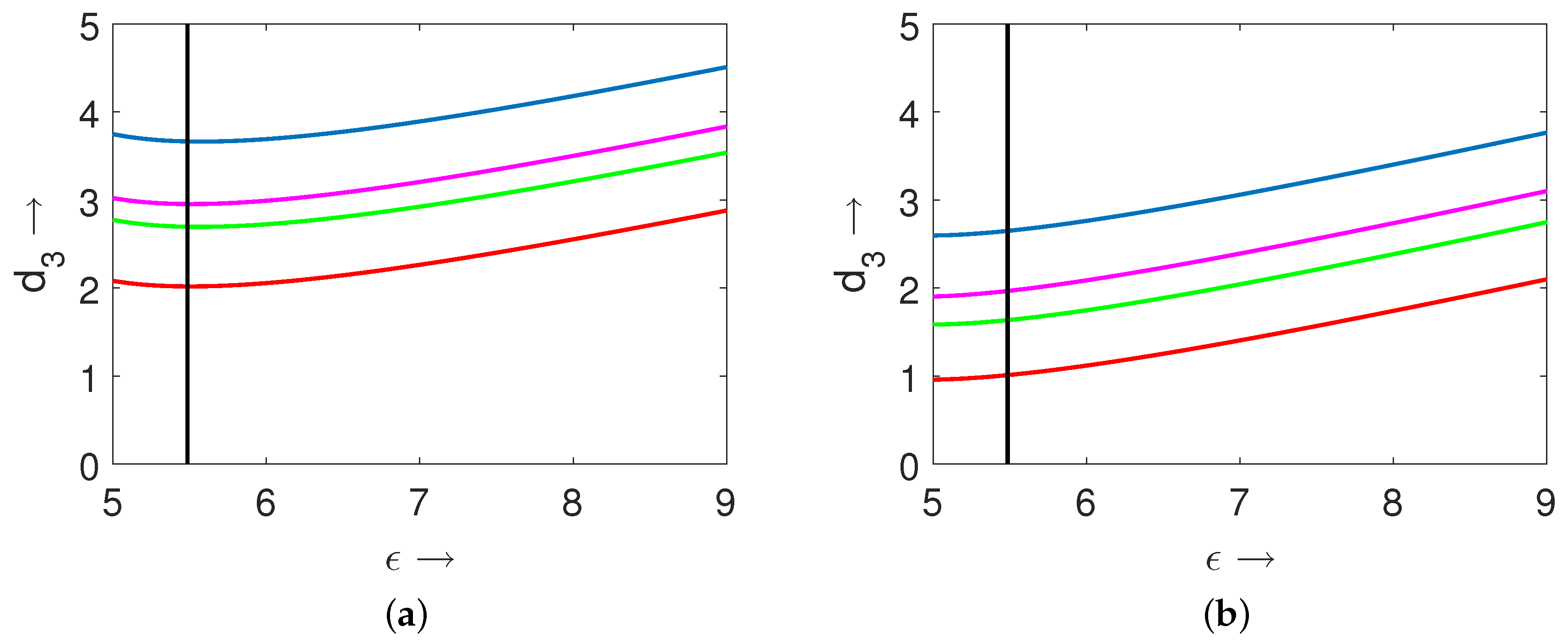In these two figures, the black vertical straight line (at $ϵ=5.486$) represents the temporal-Hopf bifurcation threshold. Since the expression for the temporal-Hopf bifurcation threshold did not involve any of the diffusion coefficients, we had the exact same position for this line in both the figures for the considered two different values of $d_2$. For the both of these figures, the blue curve represents the Turing curve for the local model (i.e., ${\delta }_1={\delta }_2=0$), magenta curve represents the Turing curve for the nonlocal model where the nonlocality is incorporated only in the first prey species (i.e., ${\delta }_2=0$) with ${\delta }_1=1.0$, green curve denotes the Turing curve for the nonlocal model where the nonlocality is incorporated only in the second prey species (i.e., ${\delta }_1=0$) with ${\delta }_2=1.0$, and red curve denotes the Turing curve for the nonlocal model (27)–(29) with ${\delta }_1={\delta }_2=1.0$. From these two diagrams (i.e., Figure 14a,b), we can observe that the lower value of the parameter $d_2$ enhanced the Turing instability region significantly. Also, these figures indicate that the introduction of nonlocal intra-specific competition for both the prey species led to the enlargement of the Turing instability region. For the chosen set of parameter values, we can easily notice that incorporation of nonlocality for the second prey species had greater impact on the enlargement of the Turing instability region than that of the first prey species.

For the nonlocal system (27)–(29), we used the central difference approximation for diffusion part and forward Euler scheme for the reaction part. The nonlocal interaction terms have been numerically approximated by trapezoidal rule. For all the patterns presented in this subsection, we employed the pulse-type initial conditions (26) and the periodic boundary conditions. Now, we are interested to investigate numerically the dependence of the number of patches with high population density for the stationary patterns on the extent of nonlocality inside the Turing domain. For this purpose, we considered the parameter values $d_2=0.2$, $d_3=9.0$, $ϵ=5.0$ and the remaining parameter values as the same as above. Also, we took equal extents of nonlocality for both the prey species (that is, ${\delta }_1={\delta }_2=\delta$). 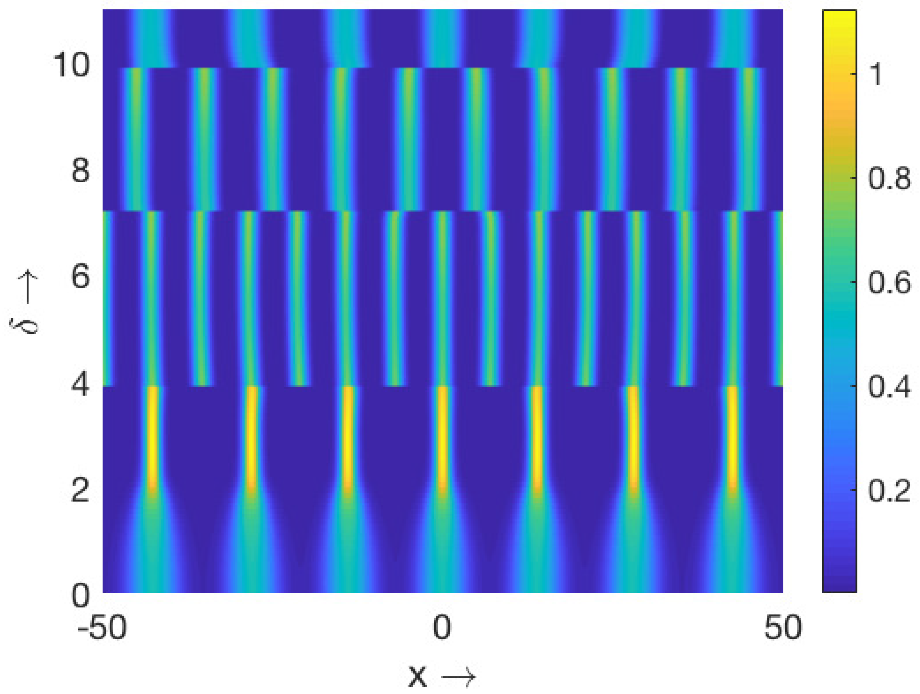We present the corresponding numerical results for the first prey species in Figure 15 over one-dimensional spatial domain $[-50,50]$. We employed forward continuation technique in order to prepare this figure. This figure indicates the existence of different regimes with different number of patches depending upon the value of $\delta$. Interestingly, the number of patches initially increased with the increment in $\delta$ and then decreased.

Further, we are interested to explore the effect of the extent of nonlocality on the dynamic patterns exhibited by the corresponding local model. In order to do so, we first considered the parameter values for the homogeneous in space and periodic in time pattern presented in Figure 5a, and varied the extent of nonlocality ($\delta$). The resulting patterns for the first prey species are presented in Figure 16. The resulting patterns suggest that small values of $\delta$ retained the spatiotemporal distribution of the populations (e.g., Figure 16a for $\delta =0.5$), a slight increment in $\delta$ altered the spatiotemporal distribution by giving rise to periodic in both the space and time population distribution (e.g., Figure 16b for $\delta =0.7$), and further increments in $\delta$ resulted in the emergence of the stationary periodic in space population distribution (e.g., Figure 16c for $\delta =0.8$). The dynamic nature of the patterns presented in Figure 16a,b can be easily understood from the phase portraits illustrated in Figure 17.

Now, we considered the parameter values for the chaotic pattern presented in Figure 8a, and varied the value of $\delta$ to observe the effect of it on the chaotic dynamics of the local model. The corresponding numerical simulations suggest that the smaller values of $\delta$ were unable to alter the chaotic nature of the population distribution, however, interestingly destroyed the symmetry observed for the local model (e.g., Figure 18a for $\delta =1.0$). A gradual increment in $\delta$ resulted in a chaotic pattern where long patches broke into smaller patches (e.g., Figure 18b for $\delta =2.0$), and finally settled into a stationary periodic in space pattern for higher values of $\delta$ (e.g., Figure 18c for $\delta =2.5$). Chaotic nature of the patterns presented in Figure 18a,b can be easily observed from the phase portraits illustrated in Figure 19. The chaotic nature of these patterns have also been cross verified by checking the sensitivity to initial conditions as described in [59], but we do not present the results here for the sake of brevity. For the intermediate periodic in both the space and time population distributions presented in Figure 5b and Figure 8b, we found that the small extents of nonlocality for both the prey species could potentially stabilize the population distributions by giving rise to the stationary periodic in space distributions and we chose not to display these results here for the sake of brevity. Overall, the above observations indicate the stabilizing effect of the extents of nonlocality for all the three considered species.

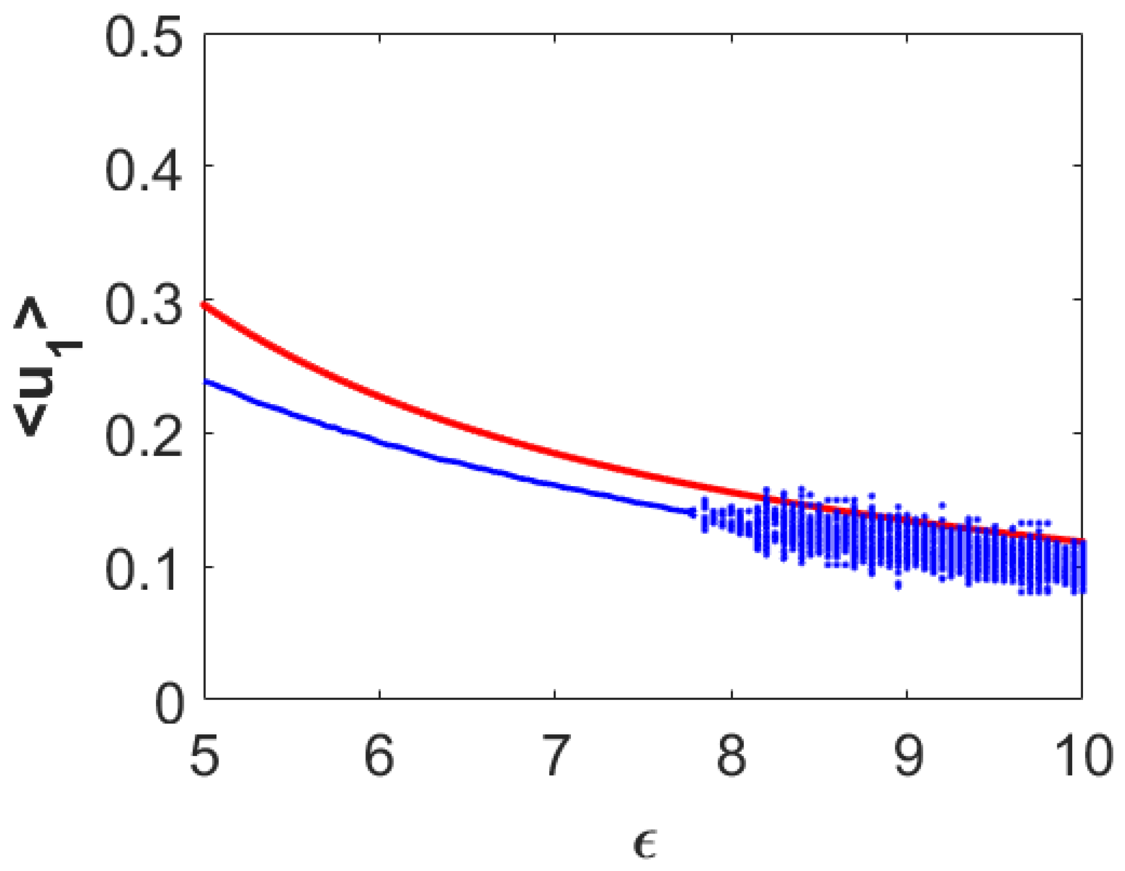
Finally, we want to explore the effects of the extent of nonlocality on the dynamics presented in Figure 1 and Figure 11. For this purpose, we considered the same parameter values as it was used to prepare the bifurcation diagram presented in Figure 11 with ${\delta }_1={\delta }_2=2.0$. The resulting dynamics are encapsulated in Figure 20. In this figure, the red colored curve corresponds to the first prey component from the spatially homogeneous coexistence steady state and blue color stands for the simulation results of the nonlocal model (27)–(29). Here, we can observe that the average densities of the first prey species stayed almost below the steady state values throughout the region in presence of the nonlocal interactions. Also, note that spatial heterogeneity in population distribution appeared throughout the region as opposed to that for both the temporal and local spatiotemporal cases. This figure reconfirms that the spatially heterogeneous population distribution can suppress the spatially averaged density for the first prey species. The same scenario happens for the second prey species, whereas, the spatial heterogeneity enhances the spatially averaged density for the predator population. For the sake of brevity, we restrict ourselves from displaying the corresponding bifurcation diagrams for both the second prey and predator species.

5. Discussion

The number of studies on spatiotemporal pattern formation for three-species models is comparatively less in existing literature and there exist even fewer works for models with nonlocal interactions. In this article, we have investigated for the possible impacts of random dispersal and nonlocal intra-specific interactions on the dynamics of a two-prey-one-predator system. For the temporal version of the model, we have mentioned the period-doubling route to chaos by means of numerical simulations. For the corresponding spatiotemporal models with both the local and nonlocal intra-specific interactions for the two considered prey species, we have derived the conditions for Turing instability through linear analysis. Further, we have carried out extensive numerical simulations in order to validate our theoretical predictions as well as to explore rich complex spatiotemporal dynamical behaviors which are beyond the scope of linear analysis. Overall, we have presented a comparative study on the dynamics possessed by the temporal, local, and nonlocal spatiotemporal models.

Local spatiotemporal model (11)–(13) along with the periodic boundary conditions possesses a wide variety of stationary and dynamic patterns. For the parameter values well inside the Turing domain, the model produces stationary periodic in space patterns for all the three considered species. However, an interesting phenomenon has been observed for these stationary patterns where the regions with high first prey density correspond to the same for predator but to low second prey density. This phenomenon arises due to the fact that the chosen values of the parameter $ϵ$ are much large than the parameter $\mu$ and this makes the first prey species more favorable to predator than the second prey species. Apart from this, numerical simulations show the stabilizing effect of diffusion on the spatial population distributions by making the periodic in time homogeneous in space or even chaotic population distributions to stationary periodic in space one for higher values of diffusion coefficient of predator species ($d_3$). Both these transitions occur through the periodic in both space and time population distribution for intermediate values of $d_3$. We would like to mention here that the choice of other diffusion coefficients as bifurcation parameter will not reveal any additional feature as the main determining factor is the location of the parameter value with respect to the temporal-Hopf and Turing bifurcation curves.

Traditionally, the spatiotemporal dynamics of an ecological system have been investigated in the asymptotic sense. Sometimes it can take a very long time period for an ecological system to eventually settle down to a spatiotemporal state and this long time period can be as long as a few generations for certain species. Therefore, from the perspective of ecological time scales it is very important to investigate the quasi-stable transients for an ecological system and to identify the key factors for its appearance [60]. A long transient exhibits a quasi-stable dynamics for a few generations and then the ecological system experiences an abrupt transition to another regime [60]. Hence, it can provide an alternative explanation for ecological regime shifts apart from the usual concept of bifurcation [60]. However, bifurcation of dynamical behaviors for a system arises due to directional change in parameter values (for example, Figure 7 and Figure 11) and this directional change is often considered to be mediated through external factors, such as climate change [60]. Therefore, bifurcation can provide useful explanation for exogenously triggered regime shifts whereas long transients can serve as alternative underlying mechanisms for regime shifts [60]. Hence, the bifurcation diagrams such as Figure 7 and Figure 11 exhibit exogenously triggered regime shifts while the phase portraits presented in Figure 10 provide evidence for endogenously triggered regime shift for the local spatiotemporal model (11)–(13).

Further, we have investigated for the possible effects of random dispersal of all the considered species on the dynamics possessed by the corresponding temporal model. In this regard, we have observed that the local spatiotemporal model (11)–(13) with spatially homogeneous initial conditions preserves the temporal dynamics whereas the system with pulse type initial conditions produces smaller amplitude chaotic oscillations than the temporal chaos. This type of reduction in amplitude of chaotic oscillations arises due to the emergence of spatial heterogeneity in population distributions. It is worthy to mention here that the spatially homogeneous perturbation over the entire domain is not ecologically realistic. Therefore, our results suggest that one should expect small amplitude chaotic oscillations for a spatially heterogeneous population as compared to a spatially homogeneous population. Also, we have shown that the backward continuation technique significantly enhances the spatially heterogeneous chaotic regime by destroying the period-doubling route to chaos. These bifurcation diagrams (that is, Figure 1, Figure 11 and Figure 12) vouch for the existence of alternative stable states for the spatiotemporal model without nonlocal interactions (11)–(13).

Another interesting dynamical aspect of the local spatiotemporal model (11)–(13) is that the nature of the patterns produced is not independent of the spatial domain size for certain parameter range, in particular, for parameter values in temporal-Hopf unstable region sufficiently far from the temporal-Hopf threshold. In this regard, we have shown that a chaotic pattern can become a two-periodic one in smaller spatial domain and even a stationary heterogeneous pattern can loose its stability through becoming a periodic one in both the space and time in smaller spatial domain. These spatial domain size dependence of spatiotemporal patterns have been reported in Figure 13. Therefore, our study suggests that one can get different spatiotemporal patterns depending on the spatial domain size. At this point, we would like to emphasize on the fact that this type of domain size dependence for the resulting spatiotemporal patterns is not unheard of at all. For instance, Barrio et al. [61] showed that both the domain size and shape can have significant roles in selection of different types of patterns. Also, Neville et al. [62] investigated how domain growth can influence pattern formation. Hence, our findings on domain size dependence of patterns are in accordance with literature and carry forward our understanding in this direction.

The dependence of results on the domain size can be explained as follows. If there exists a spatially periodic solution $u(x,t)$ with the wavenumber k and the length of the interval $L_1=\frac{2\pi n_1}{k}$, where $n_1\in \mathbb{N}$, then this solution can be naturally extended by periodicity to the interval $L_2=\frac{2\pi n_2}{k}$, where $n_2>n_1$. Moreover, if we increase the length of the interval, solutions with other wavenumbers can appear due to their successive bifurcations from the spatially homogeneous stationary solutions. Furthermore, solutions with a fixed wavenumber persist under the variation of the length of the interval in some range of lengths. Hence, solutions with different wavenumbers can coexist for the same length, and their number increases with the increase of L. This multiplicity of solutions is conventionally observed in bifurcation problems. Their stability and basins of attraction depend on the length L. The interaction of different solutions can result in complex dynamics including chaotic behavior. The transition from two-periodic oscillations to chaotic oscillations for a larger length (cf. Figure 8 and Figure 13) corresponds to this understanding of the dynamics of solutions. It is also possible that the initial condition remains in the basin of attraction of the same solution, such that we observe the same dynamics for a changing interval.

Finally, we have studied the effects of nonlocal interactions for both the prey species on the spatiotemporal dynamics. Our study suggests that the introduction of nonlocal interactions for both the prey species or any one of them can lead to the enlargement of the Turing instability region where nonlocality for the second prey species possess greater impact than that for the first prey species. In order to understand the impact of nonlocality on the stationary Turing patterns, we have employed forward continuation technique which shows the existence of multiple stationary regimes with different number of patches. The number of patches initially increases and then decreases with increasing extent of nonlocality. This scenario is encapsulated in Figure 15 and it is different from the result presented in [48] where the number of patches gradually increases. Another interesting feature of the dynamics of nonlocal model (27)–(29) is that it breaks the spatial symmetry possessed by local model (11)–(13) for chaotic population distribution. Our results also indicate that the nonlocality acts as a stabilizing factor as large extent of it can suppress the oscillatory behaviors by changing them to stationary patterns. Ecologically it can be interpreted as the access to the nearby resources allow the species to be confined within a patch rather than changing its position in a regular or irregular fashion. Further, our investigation suggests that the presence of spatial heterogeneity in population distributions can diminish the spatially averaged density for both the prey species (for instance, see the Figure 20 for the first prey species) and enhances the same for the predator species.

This study leads to some other interesting and relevant problems to investigate. In this study, we have confined ourselves to only the top-hat kernel function in order to model the nonlocal interactions. However, it will be a fascinating future research prospect to investigate the spatiotemporal dynamics with other types of kernel functions such as Gaussian, Laplacian and triangular kernels etc. Another interesting problem will be to consider nonlocal consumption for predator species and examine its effect on dynamics. The present study has considered Lotka–Volterra type linear functional responses in order to capture the prey–predator interactions whereas the consideration of more suited functional responses such as Holling type-II and Beddington–DeAngelis functional responses will make the investigation ecologically more viable and challenging. These interesting as well as challenging issues will be taken care of in our future works.