Linguistic Picture Fuzzy Dombi Aggregation Operators and Their Application in Multiple Attribute Group Decision Making Problem

Abstract

The aims of this study are to propose the linguistic picture fuzzy Dombi (LPFD) aggregation operators and decision-making approach to deal with uncertainties in the form of linguistic picture fuzzy sets. LPFD operators have more flexibility due to the general fuzzy set. Utilizing the Dombi operational rule, the series of Dombi aggregation operators were proposed, namely linguistic picture fuzzy Dombi arithmetic/geometric, ordered arithmetic/ordered geometric and Hybrid arithmetic/Hybrid geometric aggregation operators. The distinguished feature of these proposed operators is studied. At that point, we have used these Dombi operators to design a model to deal with multiple attribute decision-making (MADM) issues under linguistic picture fuzzy information. Finally, an illustrative example to evaluate the emerging technology enterprises is provided to demonstrate the effectiveness of the proposed approach, together with a sensitivity analysis and comparison analysis, proving that its results are feasible and credible.

1. Introduction

The intuitionistic fuzzy set (IFS) [1] has discussed only two categories of responses “yes” and “no”, but many real life problems have more then two types of responses, such that, in case of selection, we face three types of responses “yes”, “no” and “refusal”. Thus, to overcome this issue, Cuong [2,3] introduced a novel concept of picture fuzzy set (PFS), which is dignified in three different functions presenting the positive, neutral and negative membership degrees. Cuong [4] studied some characteristic of PFSs and also approved their distance measures. Cuong and Hai [5] defined firstly the fuzzy logic operators and implications functions for PFS. Cuong et al. [6] examined the characteristic of picture fuzzy t-norm and t-conorm. Phong et al. [7] examined certain configurations of PF relations. Wei et al. [8,9,10] defined many procedures to compute the closeness between PFSs. Presently, many researchers have developed more models in the PFS condition: a correlation coefficient of PFS is proposed by Sing [11] and applies it to clustering analysis. Son et al. [12,13] provided time arrangement calculation and temperature estimation on the basis of PFS domain. Son [14,15] defined picture fuzzy separation measures, generalized picture fuzzy distance measures and picture fuzzy association measures, and combined it to tackle grouping examination under PFS condition. A novel fuzzy derivation structure on PFS is defined by Son et al. [16] to improve the performance of the classical fuzzy inference system. To handle decision making problems, Ashraf et al. [17] introduced two decision techniques; firstly, they proposed a series of geometric aggregation operators and, secondly, introduced the TOPSIS method to deal with uncertainty in the form of PF sets. In addition, Ashraf et al. [18] proposed the PF linguistic set to deal with linguistic information in (decision-making) DM problems. Zeng et al. [19] proposed the exponential jensen PF divergence measure to deal with DM problems using PF information. Khan et al. [20] examined the application of a generalized PF soft set in DM problems. Khan et al. [21] introduced the Einstein aggregation operators for PF information. Thong et al. [22,23] proposed the DM approach using PF clustering to deal with uncertainty in the form of PF sets. Khan et al. [24] described the application of logarithmic aggregation operators of PF numbers in DM problems. Wei [25] proposed the series of aggregation operator to handle the decision problem using PF information. Peng et al. [26] proposed an PFS algorithm and tested it in decision-making. Bo and Zhang [27] studied some new operations of picture fuzzy relations such as type-2 inclusion relation, type-2 union, type-2 intersection and type-2 complement operations and also defined the anti-reflexive kernel, symmetric kernel, reflexive closure and symmetric closure of a picture fuzzy relation. For more detailed study, we refer to [28,29,30].

Dombi introduced [31] a new type of operations called the Dombi triangular norm and Dombi triangular conorm, demonstrating the preference of variability with the operation of parameters. For the first time in [32], Dombi operations were used for IFS to handle decision-making problems by introducing a Dombi Bonferroni mean operator. Dombi aggregation operation was further extended to a single neutrosophic set [33]. Travel decision-making problems were solved by using Dombi operations [34] by inspecting neutrosophic cubic sets. Dombi aggregation operations were further extended to linguistic cubic variables [35], Dombi hesitant fuzzy information [36] by utilizing the multi attribute decision-making methods to solve different real-life problems. Furthermore, Dombi picture fuzzy sets and aggregation operation are proposed in [37] for evaluating different significances of selections among others in the decision-making process. Bipolar fuzzy Dombi aggregation operators are introduced [38] based on arithmetic and geometric Dombi operations. Pythagorean fuzzy Dombi aggregation operators are proposed [39] for evaluating the uncertainty in decision-making problems. Application of spherical fuzzy Dombi aggregation operators is introduced [40] for evaluating the best alternative using spherical fuzzy information.

Motivated by the above discussion, we proposed the naval aggregation operators for linguistic picture fuzzy numbers using Dombi t-norm and Dombi t-conorm. The proposed operators play a vital role of aggregating the linguistic picture fuzzy information. For revelation and numerical application of the proposed operators, a numerical example is constructed. The rest of this study is designed as follows. Section 2 provides a brief overview of the basic knowledge of the extension of a linguistic fuzzy set. The novel Dombi aggregation operators are introduced in Section 3. Section 4 consists of some discussion on the application of a defined approach. In Section 5, we discussed the comparison and advantages of the proposed work and, finally, conclusions are drawn in Section 6.

2. Preliminaries

Definition 1.

([2]) Let $\widehat{H}$ be a fixed set; then, a PFS p in $\widehat{h}$ is defined as

$$p=\left\{(\widehat{h},{\hat{\alpha }}_p\left(\widehat{h}\right),{\hat{\beta }}_p\left(\widehat{h}\right),{\hat{\gamma }}_p\left(\widehat{h}\right))\right|\widehat{h}\in \widehat{H}\},$$

(1)

where${\hat{\alpha }}_p\left(\widehat{h}\right):\widehat{H}⟶[0,1],\widehat{h}\in \widehat{H}⟶{\hat{\alpha }}_p\left(\widehat{h}\right)\in [0,1];$

${\hat{\beta }}_p\left(\widehat{h}\right):\widehat{H}⟶[0,1],\widehat{h}\in \widehat{H}⟶{\hat{\beta }}_p\left(\widehat{h}\right)\in [0,1];{\hat{\gamma }}_p\left(\widehat{h}\right):\widehat{H}⟶[0,1],$

$\widehat{h}\in \widehat{H}⟶{\hat{\alpha }}_p\left(\widehat{h}\right)\in [0,1]$satisfies the condition: $0\le {\hat{\alpha }}_p\left(\widehat{h}\right),{\hat{\beta }}_p\left(\widehat{h}\right),{\hat{\gamma }}_p\left(\widehat{h}\right)\le 1.$ Furthermore, ${\hat{\alpha }}_p\left(\widehat{h}\right),{\hat{\beta }}_p\left(\widehat{h}\right)$ and ${\hat{\gamma }}_p\left(\widehat{h}\right)$ indicate the positive, neutral and negative grads of the element $\widehat{h}\in \widehat{H}$ to the set $p,$ respectively. For each PFS, $p\subseteq \widehat{H},{\pi }_p\left(\widehat{h}\right)=1-{\hat{\alpha }}_p\left(\widehat{h}\right)-{\hat{\beta }}_p\left(\widehat{h}\right)-{\hat{\gamma }}_p\left(\widehat{h}\right)$ is said to be the refusal degree of $\widehat{H}$ to $p.$

Definition 2.

([2,25]) Let $p=({\hat{\alpha }}_p\left(\widehat{h}\right),{\hat{\beta }}_p\left(\widehat{h}\right),{\hat{\gamma }}_p\left(\widehat{h}\right))$ and $\mathbb{Q}=({\hat{\alpha }}_{\mathbb{Q}}\left(\widehat{h}\right),{\hat{\beta }}_{\mathbb{Q}}\left(\widehat{h}\right),{\hat{\gamma }}_{\mathbb{Q}}\left(\widehat{h}\right))$ be two PFNs on the universe $\widehat{h}.$ Then, the operation laws between p and $\mathbb{Q}$ are stated as:

(1) $p\subseteq \mathbb{Q},$ if ${\hat{\alpha }}_p\left(\widehat{h}\right)\le {\hat{\alpha }}_{\mathbb{Q}}\left(\widehat{h}\right),{\hat{\beta }}_p\left(\widehat{h}\right)\le {\hat{\beta }}_{\mathbb{Q}}\left(\widehat{h}\right)$ and ${\hat{\gamma }}_p\left(\widehat{h}\right)\ge {\hat{\gamma }}_{\mathbb{Q}}\left(\widehat{h}\right)\forall \widehat{h}\in \widehat{H};$

(2) $p=\mathbb{Q}$ iff $p\subseteq \mathbb{Q}$ and $p\supseteq \mathbb{Q};$

(3) $p\cup \mathbb{Q}=\left\{\begin{array}{c}〈(\widehat{h},max\{{\hat{\alpha }}_p\left(\widehat{h}\right),{\hat{\alpha }}_{\mathbb{Q}}\left(\widehat{h}\right)\},min\{{\hat{\beta }}_p\left(\widehat{h}\right),{\hat{\beta }}_{\mathbb{Q}}\left(\widehat{h}\right)\},min\{{\hat{\gamma }}_p\left(\widehat{h}\right),{\hat{\gamma }}_{\mathbb{Q}}\left(\widehat{h}\right))〉\\ |\widehat{h}\in \widehat{H}\end{array}\right\};$

(4) $p\cap \mathbb{Q}=\left\{\begin{array}{c}(\widehat{h},min\{{\hat{\alpha }}_p\left(\widehat{h}\right),{\hat{\alpha }}_{\mathbb{Q}}\left(\widehat{h}\right)\},max\{{\hat{\beta }}_p\left(\widehat{h}\right),{\hat{\beta }}_{\mathbb{Q}}\left(\widehat{h}\right)\},max\{{\hat{\gamma }}_p\left(\widehat{h}\right),{\hat{\gamma }}_{\mathbb{Q}}\left(\widehat{h}\right))\\ |\widehat{h}\in \widehat{H}\end{array}\right\};$

(5) $p^{/}=\left({\hat{\gamma }}_p\left(\widehat{h}\right),{\hat{\beta }}_p\left(\widehat{h}\right),{\hat{\alpha }}_p\left(\widehat{h}\right)\right);$

(6) $p\oplus \mathbb{Q}=\left({\hat{\alpha }}_p\left(\widehat{h}\right)+{\hat{\alpha }}_{\mathbb{Q}}\left(\widehat{h}\right)-{\hat{\alpha }}_p\left(\widehat{h}\right).{\hat{\alpha }}_{\mathbb{Q}}\left(\widehat{h}\right),{\hat{\beta }}_p\left(\widehat{h}\right).{\hat{\beta }}_{\mathbb{Q}}\left(\widehat{h}\right),{\hat{\gamma }}_p\left(\widehat{h}\right),{\hat{\gamma }}_{\mathbb{Q}}\left(\widehat{h}\right)\right);$

(7) $p\otimes \mathbb{Q}=\left(\begin{array}{c}{\hat{\alpha }}_p\left(\widehat{h}\right).{\hat{\alpha }}_{\mathbb{Q}}\left(\widehat{h}\right),{\hat{\beta }}_p\left(\widehat{h}\right)+{\hat{\beta }}_{\mathbb{Q}}\left(\widehat{h}\right)-{\hat{\beta }}_p\left(\widehat{h}\right).{\hat{\beta }}_{\mathbb{Q}}\left(\widehat{h}\right),{\hat{\gamma }}_p\left(\widehat{h}\right)\\ +{\hat{\gamma }}_{\mathbb{Q}}\left(\widehat{h}\right)-{\hat{\gamma }}_p\left(\widehat{h}\right),{\hat{\gamma }}_{\mathbb{Q}}\left(\widehat{h}\right)\end{array}\right);$

(8) $\lambda p=\left(1-{(1-{\hat{\alpha }}_p\left(\widehat{h}\right))}^{\lambda },{\hat{\beta }}_p^{\lambda }\left(\widehat{h}\right),{\hat{\gamma }}_{\mathbb{Q}}^{\lambda }\left(\widehat{h}\right)\right);$

(9) $p^{\lambda }=\left({\hat{\alpha }}_p^{\lambda }\left(\widehat{h}\right),1-{(1-{\hat{\beta }}_p\left(\widehat{h}\right))}^{\lambda },1-{(1-{\hat{\gamma }}_p\left(\widehat{h}\right))}^{\lambda }\right).$

Definition 3.

([41,42]) Let $\acute{S}=({\acute{s}}_1,{\acute{s}}_2,\dots ,{\acute{s}}_t)$ be the finite and absolutely order distinct term set. Then, $\acute{S}$ is the linguistic term set, where t is the odd value, e.g., $3,5,\dots ,$ when $t=5,$ then $\acute{S}$ can be written as $\acute{S}=({\acute{s}}_1,{\acute{s}}_2,{\acute{s}}_3,{\acute{s}}_4,{\acute{s}}_5)=$ ( poor, slightly poor, fair, slightly good, good)

The following characteristics of the linguistic set $\acute{S}$ must be satisfied:

(1) Ordered $:{\acute{s}}_k\prec {\acute{s}}_l,\iff k\prec l;$

(2) Negation: neg $\left({\acute{s}}_k\right)={\acute{s}}_{t-1-k};$

(3) Max: $({\acute{s}}_k,{\acute{s}}_l)={\acute{s}}_k,$ iff $k\ge l;$

(4) Min: $({\acute{s}}_k,{\acute{s}}_l)={\acute{s}}_k,$ iff $k\le l.$

The extended form of the discrete term set $\acute{S}$ is called a continuous linguistic term set and defined as ${\acute{S}}^{*}=\left\{{\acute{s}}_{\psi }\right|{\acute{s}}_0\le {\acute{s}}_{\psi }\le {\acute{s}}_g,\psi \in [0,t],$ and, if ${\acute{s}}_{\psi }\in {\acute{S}}^{*},$ then ${\acute{s}}_{\psi }$ is called the original term otherwise, virtual term.

Definition 4.

([18]) Let $\widehat{H}\ne 0$ and ${\acute{S}}^{*}=\left\{{\acute{s}}_{\psi }\right|{\acute{s}}_0\le {\acute{s}}_{\psi }\le {\acute{s}}_g,\psi \in [0,t]$ be a continuous linguistic set. Then, an LPFS is defined as

$$p=\left\{〈\widehat{h},{\acute{s}}_{\theta }\left(\widehat{h}\right),{\acute{s}}_{\tau }\left(\widehat{h}\right),{\acute{s}}_{\sigma }\left(\widehat{h}\right)〉\right|\widehat{h}\in \widehat{H}\},$$

(2)

where $〈{\acute{s}}_{\theta }\left(\widehat{h}\right),{\acute{s}}_{\tau }\left(\widehat{h}\right),{\acute{s}}_{\sigma }\left(\widehat{h}\right)〉\in {\acute{s}}^{*}$ stands for the linguistic positive, linguistic neutral and linguistic negative degrees of the element $\widehat{H}$ to $p.$ We shall denote the triple of $〈{\acute{s}}_{\theta }\left(\widehat{h}\right),{\acute{s}}_{\tau }\left(\widehat{h}\right),{\acute{s}}_{\sigma }\left(\widehat{h}\right)〉$ as $p=〈{\acute{s}}_{\theta },{\acute{s}}_{\tau },{\acute{s}}_{\sigma }〉$ and referred to as linguistic picture fuzzy value (LPFV).

For any $\widehat{h}\in \widehat{h},$ the condition $\theta +\tau +\sigma \le t$ is always satisfied, and $\pi \left(\widehat{h}\right)={\acute{s}}_{t-\theta -\tau -\sigma }$ is the linguistic refusal degree of $\widehat{h}$ to $p.$ Obviously, if $\theta -\tau -\sigma =t,$ then LPFS has the minimum linguistic indeterminacy degree, that is,$\pi \left(\widehat{h}\right)={\acute{s}}_0,$ which means the membership degree of $\widehat{h}$ to p can be precisely expressed with a single linguistic term and LPFS p is reduced to a linguistic variable. On the contrary, if $\theta =\tau =\sigma =0,$ then LPFS $A\left(\widehat{h}\right)$ has the maximum linguistic indeterminacy degree; that is, $\pi \left(\widehat{h}\right)={\acute{s}}_0.$

Definition 5.

([43]) If $\hat{p}=({\acute{s}}_{\theta },{\acute{s}}_{\tau },{\acute{s}}_{\sigma })$ is an LPFN, then the score index and accuracy index is defined as

$$\begin{array}{ccc}\hfill \overline{E}\left(\hat{p}\right)& =& \frac{\theta +\tau -\sigma }{t},\overline{E}\left(\hat{p}\right)\in [-1,1],\hfill \end{array}$$

(3)

$$\begin{array}{ccc}\hfill \hat{L}\left(\hat{p}\right)& =& \frac{\theta +\tau +\sigma }{t},\hat{L}\left(\hat{p}\right)\in [0,1].\hfill \end{array}$$

(4)

Definition 6.

([17]) Let $\hat{p}$ and $\hat{\mathbb{Q}}$ be the picture fuzzy numbers. Then, $\hat{p}>\hat{\mathbb{Q}}$ iff;

(1) If Ē$\left(\hat{p}\right)>$ Ē$\left(\hat{\mathbb{Q}}\right)$, then $\hat{p}$ is superior to $\hat{\mathbb{Q}}$, denoted by $\hat{p}>\hat{\mathbb{Q}};$

(2) Ē$\left(\hat{p}\right)=$ Ē$\left(\hat{\mathbb{Q}}\right)$, then

(a) $\hat{L}\left(\hat{p}\right)>\hat{L}\left(\hat{\mathbb{Q}}\right)$, implies that $\hat{p}$ is superior to $\hat{\mathbb{Q}}$, denoted by $\hat{p}>\hat{\mathbb{Q}};$

(b)$\hat{L}\left(\hat{p}\right)=\hat{L}\left(\hat{\mathbb{Q}}\right)$, implies that $\hat{p}$ is equivalent to $\hat{\mathbb{Q}}$, denoted by $\hat{p}\sim \hat{\mathbb{Q}};$

Definition 7.

([31]) Let A and B be any two real numbers. If $(A,B)\in [0,1]\times [0,1],$ then Dombi traingular-norm and triangular-conorm are defined as

$$Do(A,B)=\frac{1}{1+{\left\{{\left(\frac{1-A}{A}\right)}^{\Re }+{\left(\frac{1-B}{B}\right)}^{\Re }\right\}}^{\frac{1}{\Re }}},$$

(5)

$$D{o}^c(A,B)=1-\frac{1}{1+{\left\{{\left(\frac{A}{1-A}\right)}^{\Re }+{\left(\frac{B}{1-B}\right)}^{\Re }\right\}}^{\frac{1}{\Re }}},$$

(6)

where $\Re >0,$$Do(A,B)\in [0,1]$ and $D{o}^c(A,B)\in [0,1].$

3. Linguistic Picture Fuzzy Arithmetic Aggregation Operators

Definition 8.

Let ${\hat{p}}_1=({\acute{s}}_{{\theta }_1},{\acute{s}}_{{\tau }_1},{\acute{s}}_{{\sigma }_1})$ and ${\hat{p}}_1=({\acute{s}}_{{\theta }_2},{\acute{s}}_{{\tau }_2},{\acute{s}}_{{\sigma }_2})$ be two LPFNs, $\Re >1$ and $\lambda >0.$ Then, Dombi triangular-conorm and Dombi triangular-conorm operation of LPFNs are expressed as

(1)${\hat{p}}_1\oplus {\hat{p}}_2=\left(\begin{array}{c}\left[{\acute{s}}_{t-\frac{t}{1+{\left\{{\left(\frac{{\theta }_1}{t-{\theta }_1}\right)}^{\Re }+{\left(\frac{{\theta }_2}{t-{\theta }_2}\right)}^{\Re }\right\}}^{\frac{1}{\Re }}}}\right],\left[{\acute{s}}_{\frac{t}{1+{\left\{{\left(\frac{t-{\tau }_1}{{\tau }_1}\right)}^{\Re }+{\left(\frac{t-{\tau }_2}{{\tau }_2}\right)}^{\Re }\right\}}^{\frac{1}{\Re }}}}\right],\\ \left[{\acute{s}}_{\frac{t}{1+{\left\{{\left(\frac{t-{\sigma }_1}{{\sigma }_1}\right)}^{\Re }+{\left(\frac{t-{\sigma }_2}{{\sigma }_2}\right)}^{\Re }\right\}}^{\frac{1}{\Re }}}}\right]\end{array}\right)$

(2) ${\hat{p}}_1\otimes {\hat{p}}_2=\left(\begin{array}{c}\left[{\acute{s}}_{\frac{t}{1+{\left\{{\left(\frac{t-{\theta }_1}{{\theta }_1}\right)}^{\Re }+{\left(\frac{t-{\theta }_2}{{\theta }_2}\right)}^{\Re }\right\}}^{\frac{1}{\Re }}}}\right],\left[{\acute{s}}_{t-\frac{t}{1+{\left\{{\left(\frac{{\tau }_1}{t-{\tau }_1}\right)}^{\Re }+{\left(\frac{{\tau }_2}{t-{\tau }_2}\right)}^{\Re }\right\}}^{\frac{1}{\Re }}}}\right],\\ \left[{\acute{s}}_{{}_{t-\frac{t}{1+{\left\{{\left(\frac{{\sigma }_1}{t-{\sigma }_1}\right)}^{\Re }+{\left(\frac{{\sigma }_2}{t-{\sigma }_2}\right)}^{\Re }\right\}}^{\frac{1}{\Re }}}}}\right]\end{array}\right)$

(3) $\lambda {\widehat{.p}}_1=\left(\begin{array}{c}\left[{\acute{s}}_{t-\frac{t}{1+{\left\{\lambda {\left(\frac{{\theta }_1}{t-{\theta }_1}\right)}^{\Re }\right\}}^{\frac{1}{\Re }}}}\right],\left[{\acute{s}}_{{}_{\frac{t}{1+{\left\{\lambda {\left(\frac{t-{\tau }_1}{{\tau }_1}\right)}^{\Re }\right\}}^{\frac{1}{\Re }}}}}\right],\\ \left[{\acute{s}}_{\frac{t}{1+{\left\{\lambda {\left(\frac{t-{\sigma }_1}{{\sigma }_1}\right)}^{\Re }\right\}}^{\frac{1}{\Re }}}}\right]\end{array}\right)$

(4) ${\hat{p}}_1^{\lambda }=\left(\begin{array}{c}\left[{\acute{s}}_{\frac{t}{1+{\left\{\lambda {\left(\frac{t-{\theta }_1}{{\theta }_1}\right)}^{\Re }\right\}}^{\frac{1}{\Re }}}}\right],\left[{\acute{s}}_{t-\frac{t}{1+{\left\{\lambda {\left(\frac{{\tau }_1}{t-{\tau }_1}\right)}^{\Re }\right\}}^{\frac{1}{\Re }}})}\right],\\ \left[{\acute{s}}_{t-\frac{t}{1+{\left\{\lambda {\left(\frac{{\sigma }_1}{t-{\sigma }_1}\right)}^{\Re }\right\}}^{\frac{1}{\Re }}}}\right]\end{array}\right).$

Example 1.

Let ${\hat{p}}_1=({\acute{s}}_3,{\acute{s}}_2,{\acute{s}}_5)$ and ${\hat{p}}_2=({\acute{s}}_6,{\acute{s}}_3,{\acute{s}}_3)\in {\Lambda }_{[0,9]},$ be two LPFNs, then utilizing the Dombi operation defined in Definition 8 for $\Re =1,$ and $\lambda =0.5,$ we get

(1)$\begin{array}{cc}\hfill {\hat{p}}_1\oplus {\hat{p}}_2& =\left(\begin{array}{c}{\acute{s}}_{9-\frac{9}{1+{\left\{{\left(\frac{3}{9-3}\right)}^1+{\left(\frac{6}{9-6}\right)}^1\right\}}^{\frac{1}{1}}}},{\acute{s}}_{\frac{9}{1+{\left\{{\left(\frac{9-2}{2}\right)}^1+{\left(\frac{9-3}{3}\right)}^1\right\}}^{\frac{1}{1}}}},\\ {\acute{s}}_{\frac{9}{1+{\left\{{\left(\frac{9-5}{5}\right)}^1+{\left(\frac{9-3}{3}\right)}^1\right\}}^{\frac{1}{1}}}}\end{array}\right)\hfill \\ & \hfill =〈{\acute{s}}_{6.43},{\acute{s}}_{7.62},{\acute{s}}_{6.64}〉\end{array}$

(2)$\begin{array}{cc}\hfill {\hat{p}}_1\oplus {\hat{p}}_2& =\left(\begin{array}{c}{\acute{s}}_{\frac{9}{1+{\left\{{\left(\frac{9-3}{3}\right)}^1+{\left(\frac{9-6}{6}\right)}^1\right\}}^{\frac{1}{1}}}},{\acute{s}}_{9-\frac{9}{1+{\left\{{\left(\frac{2}{9-2}\right)}^1+{\left(\frac{3}{9-3}\right)}^1\right\}}^{\frac{1}{1}}}},\\ {\acute{s}}_{9-\frac{9}{1+{\left\{{\left(\frac{5}{9-5}\right)}^1+{\left(\frac{3}{9-3}\right)}^1\right\}}^{\frac{1}{1}}}}\end{array}\right)\hfill \\ & =〈{\acute{s}}_{2.57},{\acute{s}}_{3.94},{\acute{s}}_{5.72}〉\hfill \end{array}$

(3)$\begin{array}{cc}\hfill 0.5.{\hat{p}}_1& =\left(\begin{array}{c}{\acute{s}}_{9-\frac{9}{1+{\left\{0.5{\left(\frac{3}{9-3}\right)}^1\right\}}^{\frac{1}{1}}}},{\acute{s}}_{\frac{9}{1+{\left\{0.5{\left(\frac{9-2}{2}\right)}^1\right\}}^{\frac{1}{1}}}},\\ {\acute{s}}_{\frac{9}{1+{\left\{0.5{\left(\frac{9-5}{5}\right)}^1\right\}}^{\frac{1}{1}}}}\end{array}\right)\hfill \\ & =〈{\acute{s}}_{1.80},{\acute{s}}_{3.27},{\acute{s}}_{6.42}〉\hfill \end{array}$

(4)$\begin{array}{cc}\hfill {\hat{p}}_1^{0.5}& =\left(\begin{array}{c}{\acute{s}}_{\frac{9}{1+{\left\{0.5{\left(\frac{9-3}{3}\right)}^1\right\}}^{\frac{1}{1}}}},{\acute{s}}_{9-\frac{9}{1+{\left\{0.5{\left(\frac{2}{9-2}\right)}^1\right\}}^{\frac{1}{1}}}},\\ {\acute{s}}_{9-\frac{9}{1+{\left\{0.5{\left(\frac{5}{9-5}\right)}^1\right\}}^{\frac{1}{1}}}}\end{array}\right).\hfill \\ & =〈{\acute{s}}_{4.50},{\acute{s}}_{1.12},{\acute{s}}_{3.47}〉\hfill \end{array}$

Theorem 1.

Let $\hat{p}=({\acute{s}}_{\theta },{\acute{s}}_{\tau },{\acute{s}}_{\sigma }),{\hat{p}}_1=({\acute{s}}_{{\theta }_1},{\acute{s}}_{{\tau }_1},{\acute{s}}_{{\sigma }_1})$ and ${\hat{p}}_1=({\acute{s}}_{{\theta }_2},{\acute{s}}_{{\tau }_2},{\acute{s}}_{{\sigma }_2})$ be two LPFNs, then we have

(1) ${\hat{p}}_1\oplus {\hat{p}}_2={\hat{p}}_2\oplus {\hat{p}}_1;$

(2) ${\hat{p}}_1\otimes {\hat{p}}_2={\hat{p}}_2\otimes {\hat{p}}_1;$

(3) $\lambda ({\hat{p}}_1\oplus {\hat{p}}_2)=\lambda {\hat{p}}_2\oplus {\widehat{\lambda p}}_1,\lambda >0;$

(4) $({\lambda }_1\oplus {\lambda }_2)\hat{p}={\lambda }_1\hat{p}\oplus {\lambda }_2\hat{p},{\lambda }_1,{\lambda }_2>0;$

(5) ${({\hat{p}}_1\otimes {\hat{p}}_2)}^{\lambda }={\hat{p}}_1^{\lambda }\otimes {\hat{p}}_2^{\lambda },\lambda >0;$

(6) ${\hat{p}}^{{\lambda }_1}\otimes {\hat{p}}^{{\lambda }_2}={\hat{p}}^{({\lambda }_1+{\lambda }_2)},{\lambda }_1,{\lambda }_2>0.$

Proof. 

(1) By Definition 8, we can write

$${\hat{p}}_1\oplus {\hat{p}}_2=\left(\begin{array}{c}\left[{\acute{s}}_{t-\frac{t}{1+{\left\{{\left(\frac{{\theta }_1}{t-{\theta }_1}\right)}^{\Re }+{\left(\frac{{\theta }_2}{t-{\theta }_2}\right)}^{\Re }\right\}}^{\frac{1}{\Re }}}}\right],\left[{\acute{s}}_{\frac{t}{1+{\left\{{\left(\frac{t-{\tau }_1}{{\tau }_1}\right)}^{\Re }+{\left(\frac{t-{\tau }_2}{{\tau }_2}\right)}^{\Re }\right\}}^{\frac{1}{\Re }}}}\right],\\ \left[{\acute{s}}_{\frac{t}{1+{\left\{{\left(\frac{t-{\sigma }_1}{{\sigma }_1}\right)}^{\Re }+{\left(\frac{t-{\sigma }_2}{{\sigma }_2}\right)}^{\Re }\right\}}^{\frac{1}{\Re }}}}\right]\end{array}\right)$$

$$=\left(\begin{array}{c}\left[{\acute{s}}_{t-\frac{t}{1+{\left\{{\left(\frac{{\theta }_2}{t-{\theta }_2}\right)}^{\Re }+{\left(\frac{{\theta }_1}{t-{\theta }_1}\right)}^{\Re }\right\}}^{\frac{1}{\Re }}}}\right],\left[{\acute{s}}_{{}_{\frac{t}{1+{\left\{{\left(\frac{t-{\tau }_2}{{\tau }_2}\right)}^{\Re }+{\left(\frac{t-{\tau }_1}{{\tau }_1}\right)}^{\Re }\right\}}^{\frac{1}{\Re }}}}}\right],\\ \left[{\acute{s}}_{\frac{t}{1+{\left\{{\left(\frac{t-{\sigma }_2}{{\sigma }_2}\right)}^{\Re }+{\left(\frac{t-{\sigma }_1}{{\sigma }_1}\right)}^{\Re }\right\}}^{\frac{1}{\Re }}}}\right]\end{array}\right)$$

$$={\hat{p}}_2\oplus {\hat{p}}_1$$

(2) It is obvious.

(3) Let $\lambda ({\hat{p}}_1\oplus {\hat{p}}_2)=\lambda \left(\begin{array}{c}\left[{\acute{s}}_{t-\frac{t}{1+{\left\{{\left(\frac{{\theta }_1}{t-{\theta }_1}\right)}^{\Re }+{\left(\frac{{\theta }_2}{t-{\theta }_2}\right)}^{\Re }\right\}}^{\frac{1}{\Re }}}}\right],\left[{\acute{s}}_{\frac{t}{1+{\left\{{\left(\frac{t-{\tau }_1}{{\tau }_1}\right)}^{\Re }+{\left(\frac{t-{\tau }_2}{{\tau }_2}\right)}^{\Re }\right\}}^{\frac{1}{\Re }}}}\right],\\ \left[{\acute{s}}_{\frac{t}{1+{\left\{{\left(\frac{t-{\sigma }_1}{{\sigma }_1}\right)}^{\Re }+{\left(\frac{t-{\sigma }_2}{{\sigma }_2}\right)}^{\Re }\right\}}^{\frac{1}{\Re }}}}\right]\end{array}\right)$

$=\left(\begin{array}{c}\left[{\acute{s}}_{t-\frac{t}{1+{\left\{\lambda {\left(\frac{{\theta }_1}{t-{\theta }_1}\right)}^{\Re }+\lambda {\left(\frac{{\theta }_2}{t-{\theta }_2}\right)}^{\Re }\right\}}^{\frac{1}{\Re }}}}\right],\left[{\acute{s}}_{\frac{t}{1+{\left\{\lambda {\left(\frac{t-{\tau }_1}{{\tau }_1}\right)}^{\Re }+\lambda {\left(\frac{t-{\tau }_2}{{\tau }_2}\right)}^{\Re }\right\}}^{\frac{1}{\Re }}}}\right],\\ \left[{\acute{s}}_{\frac{t}{1+{\left\{\lambda {\left(\frac{t-{\sigma }_1}{{\sigma }_1}\right)}^{\Re }+\lambda {\left(\frac{t-{\sigma }_2}{{\sigma }_2}\right)}^{\Re }\right\}}^{\frac{1}{\Re }}}}\right]\end{array}\right)$

Now, $\lambda {\hat{p}}_1\oplus {\widehat{\lambda p}}_2=\left(\begin{array}{c}\left[{\acute{s}}_{t-\frac{t}{1+{\left\{\lambda {\left(\frac{{\theta }_1}{t-{\theta }_1}\right)}^{\Re }\right\}}^{\frac{1}{\Re }}}}\right],\left[{\acute{s}}_{\frac{t}{1+{\left\{\lambda {\left(\frac{t-{\tau }_1}{{\tau }_1}\right)}^{\Re }\right\}}^{\frac{1}{\Re }}}}\right],\\ \left[{\acute{s}}_{\frac{t}{1+{\left\{\lambda {\left(\frac{t-{\sigma }_1}{{\sigma }_1}\right)}^{\Re }\right\}}^{\frac{1}{\Re }}}}\right]\end{array}\right)$

$\oplus \left(\begin{array}{c}\left[{\acute{s}}_{t-\frac{t}{1+{\left\{\lambda {\left(\frac{{\theta }_2}{t-{\theta }_2}\right)}^{\Re }\right\}}^{\frac{1}{\Re }}}}\right],\left[{\acute{s}}_{\frac{t}{1+{\left\{\lambda {\left(\frac{t-{\tau }_2}{{\tau }_2}\right)}^{\Re }\right\}}^{\frac{1}{\Re }}}}\right],\\ \left[{\acute{s}}_{\frac{t}{1+{\left\{\lambda {\left(\frac{t-{\sigma }_2}{{\sigma }_2}\right)}^{\Re }\right\}}^{\frac{1}{\Re }}}}\right]\end{array}\right)$

$=\left(\begin{array}{c}\left[{\acute{s}}_{t-\frac{t}{1+{\left\{\lambda {\left(\frac{{\theta }_1}{t-{\theta }_1}\right)}^{\Re }+\lambda {\left(\frac{{\theta }_2}{t-{\theta }_2}\right)}^{\Re }\right\}}^{\frac{1}{\Re }}}}\right],\left[{\acute{s}}_{\frac{t}{1+{\left\{\lambda {\left(\frac{t-{\tau }_1}{{\tau }_1}\right)}^{\Re }+\lambda {\left(\frac{t-{\tau }_2}{{\tau }_2}\right)}^{\Re }\right\}}^{\frac{1}{\Re }}}}\right],\\ \left[{\acute{s}}_{\frac{t}{1+{\left\{\lambda {\left(\frac{t-{\sigma }_1}{{\sigma }_1}\right)}^{\Re }+\lambda {\left(\frac{t-{\sigma }_2}{{\sigma }_2}\right)}^{\Re }\right\}}^{\frac{1}{\Re }}}}\right]\end{array}\right)$

$=\lambda ({\hat{p}}_1\oplus {\hat{p}}_2)$

(4) ${\lambda }_1\hat{p}\oplus {\lambda }_2\hat{p}$

$=\left(\left[{\acute{s}}_{t-\frac{t}{1+{\left\{{\lambda }_1{\left(\frac{{\theta }_1}{t-{\theta }_1}\right)}^{\Re }\right\}}^{\frac{1}{\Re }}}}\right],\left[{\acute{s}}_{\frac{t}{1+{\left\{{\lambda }_1{\left(\frac{t-{\tau }_1}{{\tau }_1}\right)}^{\Re }\right\}}^{\frac{1}{\Re }}}}\right],\left[{\acute{s}}_{\frac{t}{1+{\left\{{\lambda }_1{\left(\frac{t-{\sigma }_1}{{\sigma }_1}\right)}^{\Re }\right\}}^{\frac{1}{\Re }}}}\right]\right)$

$\oplus \left(\left[{\acute{s}}_{t-\frac{t}{1+{\left\{{\lambda }_2{\left(\frac{{\theta }_1}{t-{\theta }_1}\right)}^{\Re }\right\}}^{\frac{1}{\Re }}}}\right],\left[{\acute{s}}_{\frac{t}{1+{\left\{{\lambda }_2{\left(\frac{t-{\tau }_1}{{\tau }_1}\right)}^{\Re }\right\}}^{\frac{1}{\Re }}}}\right],\left[{\acute{s}}_{\frac{t}{1+{\left\{{\lambda }_2{\left(\frac{t-{\sigma }_1}{{\sigma }_1}\right)}^{\Re }\right\}}^{\frac{1}{\Re }}}}\right]\right)$

$=\left(\begin{array}{c}\left[{\acute{s}}_{t-\frac{t}{1+{\left\{({\lambda }_1+{\lambda }_2){\left(\frac{{\theta }_1}{t-{\theta }_1}\right)}^{\Re }\right\}}^{\frac{1}{\Re }}}}\right],\left[{\acute{s}}_{\frac{t}{1+{\left\{({\lambda }_1+{\lambda }_2){\left(\frac{t-{\tau }_1}{{\tau }_1}\right)}^{\Re }\right\}}^{\frac{1}{\Re }}}}\right],\\ \left[{\acute{s}}_{\frac{t}{1+{\left\{({\lambda }_1+{\lambda }_2){\left(\frac{t-{\sigma }_1}{{\sigma }_1}\right)}^{\Re }\right\}}^{\frac{1}{\Re }}}}\right]\end{array}\right)$

$=({\lambda }_1\oplus {\lambda }_2)\hat{p}$

(5) ${({\hat{p}}_1\otimes {\hat{p}}_2)}^{\lambda }=$

${\left(\begin{array}{c}\left[{\acute{s}}_{\frac{t}{1+{\left\{{\left(\frac{{\theta }_1}{t-{\theta }_1}\right)}^{\Re }+{\left(\frac{t-{\theta }_2}{{\theta }_2}\right)}^{\Re }\right\}}^{\frac{1}{\Re }}}}\right],\left[{\acute{s}}_{t-\frac{t}{1+{\left\{{\left(\frac{{\tau }_1}{t-{\tau }_1}\right)}^{\Re }+{\left(\frac{{\tau }_2}{t-{\tau }_2}\right)}^{\Re }\right\}}^{\frac{1}{\Re }}}}\right],\\ \left[{\acute{s}}_{t-\frac{t}{1+{\left\{{\left(\frac{{\sigma }_1}{t-{\sigma }_1}\right)}^{\Re }+{\left(\frac{{\sigma }_2}{t-{\sigma }_2}\right)}^{\Re }\right\}}^{\frac{1}{\Re }}}}\right]\end{array}\right)}^{\lambda }$

$\left(\begin{array}{c}\left[{\acute{s}}_{\frac{t}{1+{\left\{\lambda {\left(\frac{t-{\theta }_1}{{\theta }_1}\right)}^{\Re }+\lambda {\left(\frac{t-{\theta }_2}{{\theta }_2}\right)}^{\Re }\right\}}^{\frac{1}{\Re }}}}\right],\left[{\acute{s}}_{t-\frac{t}{1+{\left\{\lambda {\left(\frac{{\tau }_1}{1-{\tau }_1}\right)}^{\Re }+\lambda {\left(\frac{{\tau }_2}{t-{\tau }_2}\right)}^{\Re }\right\}}^{\frac{1}{\Re }}}}\right],\\ \left[{\acute{s}}_{t-\frac{t}{1+{\left\{\lambda {\left(\frac{{\sigma }_1}{t-{\sigma }_1}\right)}^{\Re }+\lambda {\left(\frac{{\sigma }_2}{t-{\sigma }_2}\right)}^{\Re }\right\}}^{\frac{1}{\Re }}}}\right]\end{array}\right)$

$\left(\begin{array}{c}\left[{\acute{s}}_{\frac{t}{1+{\left\{\lambda {\left(\frac{{\theta }_1}{t-{\theta }_1}\right)}^{\Re }\right\}}^{\frac{1}{\Re }}}}\right],\left[{\acute{s}}_{t-\frac{t}{1+{\left\{\lambda {\left(\frac{{\tau }_1}{t-{\tau }_1}\right)}^{\Re }\right\}}^{\frac{1}{\Re }}}}\right],\\ \left[{\acute{s}}_{t-\frac{t}{1+{\left\{\lambda {\left(\frac{{\sigma }_1}{t-{\sigma }_1}\right)}^{\Re }\right\}}^{\frac{1}{\Re }}}}\right]\end{array}\right)\otimes$

$\left(\begin{array}{c}\left[{\acute{s}}_{\frac{t}{1+{\left\{\lambda {\left(\frac{t-{\theta }_2}{{\theta }_2}\right)}^{\Re }\right\}}^{\frac{1}{\Re }}}}\right],\left[{\acute{s}}_{t-\frac{t}{1+{\left\{\lambda {\left(\frac{{\tau }_2}{t-{\tau }_2}\right)}^{\Re }\right\}}^{\frac{1}{\Re }}}}\right],\\ \left[{\acute{s}}_{t-\frac{t}{1+{\left\{\lambda {\left(\frac{{\sigma }_2}{t-{\sigma }_2}\right)}^{\Re }\right\}}^{\frac{1}{\Re }}}}\right]\end{array}\right)={\hat{p}}_1^{\lambda }\otimes {\hat{p}}_2^{\lambda }$

(6) ${\hat{p}}_1^{{\lambda }_1}\otimes {\hat{p}}_1^{{\lambda }_2}=\left(\begin{array}{c}\left[{\acute{s}}_{\frac{t}{1+{\left\{{\lambda }_1{\left(\frac{t-{\theta }_1}{{\theta }_1}\right)}^{\Re }\right\}}^{\frac{1}{\Re }}}}\right],\left[{\acute{s}}_{t-\frac{t}{1+{\left\{{\lambda }_1{\left(\frac{{\tau }_1}{t-{\tau }_1}\right)}^{\Re }\right\}}^{\frac{1}{\Re }}}}\right],\\ \left[{\acute{s}}_{t-\frac{t}{1+{\left\{{\lambda }_2{\left(\frac{{\sigma }_1}{t-{\sigma }_1}\right)}^{\Re }\right\}}^{\frac{1}{\Re }}}}\right]\end{array}\right)$

$\otimes \left(\begin{array}{c}\left[{\acute{s}}_{\frac{t}{1+{\left\{{\lambda }_2{\left(\frac{t-{\theta }_1}{{\theta }_1}\right)}^{\Re }\right\}}^{\frac{1}{\Re }}}}\right],\left[{\acute{s}}_{t-\frac{t}{1+{\left\{{\lambda }_2{\left(\frac{{\tau }_1}{t-{\tau }_1}\right)}^{\Re }\right\}}^{\frac{1}{\Re }}}}\right],\\ \left[{\acute{s}}_{t-\frac{t}{1+{\left\{{\lambda }_2{\left(\frac{{\sigma }_1}{t-{\sigma }_1}\right)}^{\Re }\right\}}^{\frac{1}{\Re }}}}\right]\end{array}\right)$

$=\left(\begin{array}{c}\left[{\acute{s}}_{\frac{t}{1+{\left\{({\lambda }_1+{\lambda }_2){\left(\frac{t-{\theta }_1}{{\theta }_1}\right)}^{\Re }\right\}}^{\frac{1}{\Re }}}}\right],\left[{\acute{s}}_{t-\frac{t}{1+{\left\{({\lambda }_1+{\lambda }_2){\left(\frac{{\tau }_1}{t-{\tau }_1}\right)}^{\Re }\right\}}^{\frac{1}{\Re }}}}\right],\\ \left[{\acute{s}}_{t-\frac{t}{1+{\left\{({\lambda }_1+{\lambda }_2){\left(\frac{{\sigma }_1}{t-{\sigma }_1}\right)}^{\Re }\right\}}^{\frac{1}{\Re }}}}\right]\end{array}\right)={\hat{p}}_1^{({\lambda }_1+{\lambda }_2)}.$  □

Definition 9.

Let ${\hat{p}}_k=({\acute{s}}_{{\theta }_k},{\acute{s}}_{{\tau }_k},{\acute{s}}_{{\sigma }_k})(k=1,2,\dots ,n)$ be a collection of LPFNs. Then, the linguistic picture fuzzy Dombi weighted averaging (LPFDWA) operator can be defined as

$$LPFDW{A}_{\mho }({\hat{p}}_1,{\hat{p}}_2,\dots ,{\hat{p}}_n)={\displaystyle \sum _{k=1}^n}\left({\mho }_k{\hat{p}}_k\right),$$

(7)

where the weighting vector of ${\hat{p}}_k(k=1,2,\sigma ,n)$ is $\mho ={({\mho }_1,{\mho }_2,\dots ,{\mho }_n)}^T$, with ${\mho }_k>0$ and ${\displaystyle \sum _{k=1}^n}{\mho }_k=1.$

Theorem 2.

Let ${\hat{p}}_k=({\acute{s}}_{{\theta }_k},{\acute{s}}_{{\tau }_k},{\acute{s}}_{{\sigma }_k})(k=1,2,\dots ,n)$ be a collection of LPFNs. Then, structure of linguistic picture fuzzy Dombi weighted averaging (LPFDWA) operator is defined using Dombi operation with $\Re >0;$

$$\begin{array}{c}LPFDW{A}_{\mho }({\hat{p}}_1,{\hat{p}}_2,\dots ,{\hat{p}}_n)={\displaystyle \sum _{k=1}^n}\left({\mho }_k{\hat{p}}_k\right)\hfill \\ =& \left(\begin{array}{c}\left[{\acute{s}}_{t-\frac{t}{1+{\left\{{\displaystyle \sum _{k=1}^n}{\mho }_k{\left(\frac{{\theta }_k}{t-{\theta }_k}\right)}^{\Re }\right\}}^{\frac{1}{\Re }}}}\right],\left[{\acute{s}}_{\frac{t}{1+{\left\{{\displaystyle \sum _{k=1}^n}{\mho }_k{\left(\frac{t-{\tau }_k}{{\tau }_k}\right)}^{\Re }\right\}}^{\frac{1}{\Re }}}}\right],\\ \left[{\acute{s}}_{\frac{t}{1+{\left\{{\displaystyle \sum _{k=1}^n}{\mho }_k{\left(\frac{t-{\sigma }_k}{{\sigma }_k}\right)}^{\Re }\right\}}^{\frac{1}{\Re }}}}\right]\end{array}\right),\end{array}$$

(8)

where $\mho ={({\mho }_1,{\mho }_2,\dots ,{\mho }_n)}^T$ is the weighting vector of ${\hat{p}}_k(k=1,2,\dots ,n),$ with ${\mho }_k>0$ and ${\displaystyle \sum _{k=1}^n}{\mho }_k=1.$

Proof. 

(i) If $n=2,$ then using Dombi operations of LPFNs, we write

$LPFDW{A}_{\mho }({\hat{p}}_1,{\hat{p}}_2)=({\hat{p}}_1\oplus {\hat{p}}_2)$

$=\left(\begin{array}{c}\left[{\acute{s}}_{t-\frac{t}{1+{\left\{{\left(\frac{{\theta }_1}{t-{\theta }_1}\right)}^{\Re }+{\left(\frac{{\theta }_2}{t-{\theta }_2}\right)}^{\Re }\right\}}^{\frac{1}{\Re }}}}\right],\left[{\acute{s}}_{\frac{t}{1+{\left\{{\left(\frac{t-{\tau }_1}{{\tau }_1}\right)}^{\Re }+{\left(\frac{t-{\tau }_2}{{\tau }_2}\right)}^{\Re }\right\}}^{\frac{1}{\Re }}}}\right],\\ \left[{\acute{s}}_{\frac{t}{1+{\left\{{\left(\frac{t-{\sigma }_1}{{\sigma }_1}\right)}^{\Re }+{\left(\frac{t-{\sigma }_2}{{\sigma }_2}\right)}^{\Re }\right\}}^{\frac{1}{\Re }}}}\right]\end{array}\right)$

$=\left(\begin{array}{c}\left[{\acute{s}}_{t-\frac{t}{1+{\left\{{\displaystyle \sum _{k=1}^2}{\left(\frac{{\theta }_k}{t-{\theta }_k}\right)}^{\Re }\right\}}^{\frac{1}{\Re }}}}\right],\left[{\acute{s}}_{\frac{t}{1+{\left\{{\displaystyle \sum _{k=1}^2}{\left(\frac{t-{\tau }_k}{{\tau }_k}\right)}^{\Re }\right\}}^{\frac{1}{\Re }}}}\right],\\ \left[{\acute{s}}_{\frac{t}{1+{\left\{{\displaystyle \sum _{k=1}^2}{\left(\frac{t-{\sigma }_k}{{\sigma }_k}\right)}^{\Re }\right\}}^{\frac{1}{\Re }}}}\right]\end{array}\right).$

Hence, Equation (8) is valid for $n=2.$

(ii) Assume that Equation (8) is valid for $n=w,$ then, by Equation (3), we get

$LPFDW{A}_{\mho }({\hat{p}}_1,{\hat{p}}_2,\dots ,{\hat{p}}_{\widehat{h}})={\displaystyle \sum _{k=1}^w}\left({\mho }_k{\hat{p}}_k\right)$

$=\left(\begin{array}{c}\left[{\acute{s}}_{t-\frac{t}{1+{\left\{{\displaystyle \sum _{k=1}^w}{\left(\frac{{\theta }_k}{t-{\theta }_k}\right)}^{\Re }\right\}}^{\frac{1}{\Re }}}}\right],\left[{\acute{s}}_{\frac{t}{1+{\left\{{\displaystyle \sum _{k=1}^w}{\left(\frac{t-{\tau }_k}{{\tau }_k}\right)}^{\Re }\right\}}^{\frac{1}{\Re }}}}\right],\\ \left[{\acute{s}}_{\frac{t}{1+{\left\{{\displaystyle \sum _{k=1}^w}{\left(\frac{t-{\sigma }_k}{{\sigma }_k}\right)}^{\Re }\right\}}^{\frac{1}{\Re }}}}\right]\end{array}\right).$

Now, for $n=w+1,$ then

$LPFDW{A}_{\mho }({\hat{p}}_1,{\hat{p}}_2,\dots ,{\hat{p}}_w)={\displaystyle \sum _{k=1}^w}\left({\mho }_k{\hat{p}}_k\right)\oplus {\mho }_{w+1}{\hat{p}}_{w+1}$

$=\left(\begin{array}{c}\left[{\acute{s}}_{t-\frac{t}{1+{\left\{{\displaystyle \sum _{k=1}^w}{\left(\frac{{\theta }_k}{t-{\theta }_k}\right)}^{\Re }\right\}}^{\frac{1}{\Re }}})}\right],\left[{\acute{s}}_{\frac{t}{1+{\left\{{\displaystyle \sum _{k=1}^w}{\left(\frac{t-{\tau }_k}{{\tau }_k}\right)}^{\Re }\right\}}^{\frac{1}{\Re }}}}\right],\\ \left[{\acute{s}}_{\frac{t}{1+{\left\{{\displaystyle \sum _{k=1}^w}{\left(\frac{t-{\sigma }_k}{{\sigma }_k}\right)}^{\Re }\right\}}^{\frac{1}{\Re }}}}\right]\end{array}\right)$

$\oplus \left(\begin{array}{c}\left[{\acute{s}}_{t-\frac{t}{1+{\left\{{\mho }_{\widehat{h}+1}{\left(\frac{{\theta }_{w+1}}{t-{\theta }_{w+1}}\right)}^{\Re }\right\}}^{\frac{1}{\Re }}}}\right],\left[{\acute{s}}_{\frac{t}{1+{\left\{{\mho }_{w+1}{\left(\frac{t-{\tau }_{w+1}}{{\tau }_{w+1}}\right)}^{\Re }\right\}}^{\frac{1}{\Re }}}}\right],\\ \left[{\acute{s}}_{\frac{t}{1+{\left\{{\mho }_{\widehat{h}+1}{\left(\frac{t-{\sigma }_{w+1}}{{\sigma }_{w+1}}\right)}^{\Re }\right\}}^{\frac{1}{\Re }}})}\right]\end{array}\right)$

$=\left(\begin{array}{c}\left[{\acute{s}}_{t-\frac{t}{1+{\left\{{\displaystyle \sum _{k=1}^{w+1}}{\mho }_k{\left(\frac{{\theta }_k}{t-{\theta }_k}\right)}^{\Re }\right\}}^{\frac{1}{\Re }}}}\right],\left[{\acute{s}}_{\frac{t}{1+{\left\{{\displaystyle \sum _{k=1}^{w+1}}{\mho }_k{\left(\frac{t-{\tau }_k}{{\tau }_k}\right)}^{\Re }\right\}}^{\frac{1}{\Re }}}}\right],\\ \left[{\acute{s}}_{\frac{t}{1+{\left\{{\displaystyle \sum _{k=1}^{w+1}}{\mho }_k{\left(\frac{t-{\sigma }_k}{{\sigma }_k}\right)}^{\Re }\right\}}^{\frac{1}{\Re }}}}\right]\end{array}\right).$

Thus, Equation (8) holds for $n=w+1,$ which is required.  □

Theorem 3.

(Idempotency). If ${\hat{p}}_k=({\acute{s}}_{{\theta }_k},{\acute{s}}_{{\tau }_k},{\acute{s}}_{{\sigma }_k})(k=1,2,\dots ,n)$ is a collection of LPFNs, then, ${\hat{p}}_k=\hat{p}\forall k,$ then $LPFDW{A}_{\mho }({\hat{p}}_1,{\hat{p}}_2,\dots ,{\hat{p}}_n)=\hat{p}.$

Proof. 

Since ${\hat{p}}_k=({\acute{s}}_{{\theta }_k},{\acute{s}}_{{\tau }_k},{\acute{s}}_{{\sigma }_k})(k=1,2,\dots ,n),$ then, by Equation (8), we have

$LPFDW{A}_{\mho }({\hat{p}}_1,{\hat{p}}_2,\dots ,{\hat{p}}_n)={\displaystyle \sum _{k=1}^n}\left({\mho }_k{\hat{p}}_k\right)$

$=\left(\begin{array}{c}\left[{\acute{s}}_{t-\frac{t}{1+{\left\{{\displaystyle \sum _{k=1}^n}{\mho }_k{\left(\frac{{\theta }_k}{t-{\theta }_k}\right)}^{\Re }\right\}}^{\frac{1}{\Re }}}}\right],\left[{\acute{s}}_{\frac{t}{1+{\left\{{\displaystyle \sum _{k=1}^n}{\mho }_k{\left(\frac{t-{\tau }_k}{{\tau }_k}\right)}^{\Re }\right\}}^{\frac{1}{\Re }}}}\right],\\ \left[{\acute{s}}_{\frac{t}{1+{\left\{{\displaystyle \sum _{k=1}^n}{\mho }_k{\left(\frac{t-{\sigma }_k}{{\sigma }_k}\right)}^{\Re }\right\}}^{\frac{1}{\Re }}}}\right]\end{array}\right)$

$=〈\left[{\acute{s}}_{t-\frac{t}{1+{\left\{{\left(\frac{{\theta }_k}{t-{\theta }_k}\right)}^{\Re }\right\}}^{\frac{1}{\Re }}}}\right],\left[{\acute{s}}_{\frac{t}{1+{\left\{{\left(\frac{t-{\tau }_k}{{\tau }_k}\right)}^{\Re }\right\}}^{\frac{1}{\Re }}})}\right],\left[{\acute{s}}_{\frac{t}{1+{\left\{{\left(\frac{t-{\sigma }_k}{{\sigma }_k}\right)}^{\Re }\right\}}^{\frac{1}{\Re }}}}\right]〉$

$=({\acute{s}}_{\theta },{\acute{s}}_{\tau },{\acute{s}}_{\sigma })=\hat{p}.$

Thus,

$$LPFDW{A}_{\mho }({\hat{p}}_1,{\hat{p}}_2,\dots ,{\hat{p}}_n)=\hat{p}.$$

 □

Theorem 4.

(Boundedness). Let ${\hat{p}}_k=({\acute{s}}_{{\theta }_k},{\acute{s}}_{{\tau }_k},{\acute{s}}_{{\sigma }_k})(k=1,2,\dots ,n)$ be a collection of LPFNs. Assume that ${\hat{p}}_k=min({\acute{s}}_{{\theta }_k},{\acute{s}}_{{\tau }_k},{\acute{s}}_{{\sigma }_k})=({\acute{s}}_{{\theta }_k^{-}},{\acute{s}}_{{\tau }_k^{-}},{\acute{s}}_{{\sigma }_k^{-}})$ and ${\hat{p}}_k=max({\acute{s}}_{{\theta }_k},{\acute{s}}_{{\tau }_k},{\acute{s}}_{{\sigma }_k})$ $=({\acute{s}}_{{\theta }_k^{+}},{\acute{s}}_{{\tau }_k^{+}},{\acute{s}}_{{\sigma }_k^{+}}),$ where ${\acute{s}}_{{\theta }^{-}}={min}_k\left({\acute{s}}_{{\theta }_k}\right),{\acute{s}}_{{\tau }^{-}}={max}_k\left({\acute{s}}_{{\tau }_k}\right),{\acute{s}}_{{\sigma }^{-}}={max}_k\left({\acute{s}}_{{\sigma }_k}\right),$ ${\acute{s}}_{{\theta }^{+}}={max}_k\left({\acute{s}}_{{\theta }_k}\right),$ ${\acute{s}}_{{\tau }^{+}}={min}_k\left({\acute{s}}_{{\tau }_k}\right),{\acute{s}}_{{\sigma }^{+}}={min}_k\left({\acute{s}}_{{\sigma }_k}\right).$ Then, we have

$\left[{\acute{s}}_{t-\frac{t}{1+{\left\{{\displaystyle \sum _{k=1}^n}{\mho }_k{\left(\frac{{\theta }^{-}}{t-\theta }\right)}^{\Re }\right\}}^{\frac{1}{\Re }}}}\right]\le \left[{\acute{s}}_{t-\frac{t}{1+{\left\{{\displaystyle \sum _{k=1}^n}{\mho }_k{\left(\frac{\theta }{t-\theta }\right)}^{\Re }\right\}}^{\frac{1}{\Re }}}}\right]\le \left[{\acute{s}}_{t-\frac{t}{1+{\left\{{\displaystyle \sum _{k=1}^n}{\mho }_k{\left(\frac{{\theta }^{+}}{t-{\theta }^{+}}\right)}^{\Re }\right\}}^{\frac{1}{\Re }}}}\right],$

$\left[{\acute{s}}_{t-\frac{t}{1+{\left\{{\displaystyle \sum _{k=1}^n}{\mho }_k{\left(\frac{{\tau }^{-}}{t-{\tau }^{-}}\right)}^{\Re }\right\}}^{\frac{1}{\Re }}}}\right]\le \left[{\acute{s}}_{t-\frac{t}{1+{\left\{{\displaystyle \sum _{k=1}^n}{\mho }_k{\left(\frac{\tau }{t-\tau }\right)}^{\Re }\right\}}^{\frac{1}{\Re }}}}\right]\le \left[{\acute{s}}_{t-\frac{t}{1+{\left\{{\displaystyle \sum _{k=1}^n}{\mho }_k{\left(\frac{{\tau }^{+}}{t-{\tau }^{+}}\right)}^{\Re }\right\}}^{\frac{1}{\Re }}}}\right],$

$\left[{\acute{s}}_{t-\frac{t}{1+{\left\{{\displaystyle \sum _{k=1}^n}{\mho }_k{\left(\frac{{\sigma }^{-}}{t-\sigma }\right)}^{\Re }\right\}}^{\frac{1}{\Re }}})}\right]\le \left[{\acute{s}}_{t-\frac{t}{1+{\left\{{\displaystyle \sum _{k=1}^n}{\mho }_k{\left(\frac{\sigma }{t-\sigma }\right)}^{\Re }\right\}}^{\frac{1}{\Re }}})}\right]\le \left[{\acute{s}}_{t-\frac{t}{1+{\left\{{\displaystyle \sum _{k=1}^n}{\mho }_k{\left(\frac{{\sigma }^{+}}{t-{\sigma }^{+}}\right)}^{\Re }\right\}}^{\frac{1}{\Re }}}}\right].$

Therefore,

$$\widehat{p^{-}}\le LPFDW{A}_{\mho }({\hat{p}}_1,{\hat{p}}_2,\dots ,{\hat{p}}_n)\le \widehat{p^{+}}.$$

Theorem 5.

(Monotonicity). Let ${\hat{p}}_k$ and ${\widehat{p^{/}}}_k(k=1,2,\dots ,n)$ be the two sets of LPFNs, if ${\hat{p}}_k\le {\widehat{p^{/}}}_k\forall k,$ then

$$LPFDW{A}_{\mho }({\hat{p}}_1,{\hat{p}}_2,\dots ,{\hat{p}}_n)=LPFDW{A}_{\mho }({\widehat{p^{/}}}_1,{\widehat{p^{/}}}_2,\dots ,{\widehat{p^{/}}}_n),$$

where ${\widehat{p^{/}}}_k(k=1,2,\dots ,n)$ is the permutation of ${\hat{p}}_k(k=1,2,\dots ,n).$

Definition 10.

Let ${\hat{p}}_k=({\acute{s}}_{{\theta }_k},{\acute{s}}_{{\tau }_k},{\acute{s}}_{{\sigma }_k})(k=1,2,\dots ,n)$ be a collection of LPFNs. Then, the linguistic picture fuzzy Dombi order weighted averaging (LPFDOWA) operator can be defined as

$$LPFDOW{A}_{\mho }({\hat{p}}_1,{\hat{p}}_2,\dots ,{\hat{p}}_n)={\displaystyle \sum _{k=1}^n}\left({\mho }_k{\hat{p}}_{k\left(\delta \right)}\right),$$

(9)

where $\left(\delta \right(1),\delta (2),\dots ,\delta (n\left)\right)$ is the permutation of ${\hat{p}}_k(k=1,2,\dots ,n),$ for which ${\hat{p}}_{k(\delta -1)}\ge {\hat{p}}_{\delta \left(k\right)},$ and the weighting vector of ${\hat{p}}_k(k=1,2,\dots ,n)$ are $\mho ={({\mho }_1,{\mho }_2,\dots ,{\mho }_n)}^T$, with ${\mho }_k>0$ and ${\displaystyle \sum _{k=1}^n}{\mho }_k=1.$

Theorem 6.

Let ${\hat{p}}_k=({\acute{s}}_{{\theta }_k},{\acute{s}}_{{\tau }_k},{\acute{s}}_{{\sigma }_k})(k=1,2,\dots ,n)$ be a collection of LPFNs. Then, the structure of a linguistic picture fuzzy Dombi weighted averaging (LPFDWA) operator is defined using Dombi operation with $\Re >0;$

$$\begin{array}{c}LPFDOW{A}_{\mho }({\hat{p}}_1,{\hat{p}}_2,\dots ,{\hat{p}}_n)={\displaystyle \sum _{k=1}^n}\left({\mho }_k{\hat{p}}_{k\left(\delta \right)}\right)\hfill \\ =& \left(\begin{array}{c}\left[{\acute{s}}_{t-\frac{t}{1+{\left\{{\displaystyle \sum _{k=1}^n}{\mho }_k{\left(\frac{{\theta }_{\delta \left(k\right)}}{t-{\theta }_{\delta \left(k\right)}}\right)}^{\Re }\right\}}^{\frac{1}{\Re }}}}\right],\left[{\acute{s}}_{\frac{t}{1+{\left\{{\displaystyle \sum _{k=1}^n}{\mho }_k{\left(\frac{t-{\tau }_{\delta \left(k\right)}}{{\tau }_{\delta \left(k\right)}}\right)}^{\Re }\right\}}^{\frac{1}{\Re }}}}\right],\\ \left[{\acute{s}}_{\frac{t}{1+{\left\{{\displaystyle \sum _{k=1}^n}{\mho }_k{\left(\frac{t-{\sigma }_{\delta \left(k\right)}}{{\sigma }_{\delta \left(k\right)}}\right)}^{\Re }\right\}}^{\frac{1}{\Re }}}}\right]\end{array}\right),\hfill \end{array}$$

(10)

where $\left(\delta \right(1),\delta (2),\dots ,\delta (n\left)\right)$ are the permutation of $(k=1,2,\dots ,n),$ for which ${\hat{p}}_{k(\delta -1)}\ge {\hat{p}}_{\delta \left(k\right)},$ with the corresponding weighting vector of ${\hat{p}}_k(k=1,2,\dots ,n)$ are $\mho ={({\mho }_1,{\mho }_2,\dots ,{\mho }_n)}^T$, such that ${\mho }_k>0$ and ${\displaystyle \sum _{k=1}^n}{\mho }_k=1.$

Theorem 7.

(Idempotency). If ${\hat{p}}_k=({\acute{s}}_{{\theta }_k},{\acute{s}}_{{\tau }_k},{\acute{s}}_{{\sigma }_k})(k=1,2,\dots ,n)$ is a collection of LPFNs that are all identical, i.e., ${\hat{p}}_k=\hat{p}\forall k,$ then $LPFDOW{A}_{\mho }({\hat{p}}_1,{\hat{p}}_2,\dots ,{\hat{p}}_n)=\hat{p}.$

Theorem 8.

(Boundedness). Let ${\hat{p}}_k=({\acute{s}}_{{\theta }_k},{\acute{s}}_{{\tau }_k},{\acute{s}}_{{\sigma }_k})(k=1,2,\dots ,n)$ be a collection of LPFNs. Assume that $\widehat{p^{-}}={min}_k{\hat{p}}_k,$ and $\widehat{p^{+}}={max}_k{\hat{p}}_k.$ Then,

$$\widehat{p^{-}}\le LPFDOW{A}_{\mho }({\hat{p}}_1,{\hat{p}}_2,\dots ,{\hat{p}}_n)\le \widehat{p^{+}}.$$

Theorem 9.

(Monotonicity). Let ${\hat{p}}_k$ and ${\widehat{p^{/}}}_k(k=1,2,\dots ,n)$ be the two sets of LPFNs, then

$$LPFDOW{A}_{\mho }({\hat{p}}_1,{\hat{p}}_2,\dots ,{\hat{p}}_n)=LPFDOW{A}_{\mho }({\widehat{p^{/}}}_1,{\widehat{p^{/}}}_2,\dots ,{\widehat{p^{/}}}_n),$$

where ${\widehat{p^{/}}}_k(k=1,2,\dots ,n)$ is any permutation of ${\hat{p}}_k(k=1,2,\dots ,n).$

Definition 11.

A linguistic picture fuzzy Dombi hybrid weighted averaging (LPFDHWA) operator of dimension n is a function $LPFDHWA:\widehat{p^n}\to \hat{p},$ with corresponding weight $\mho ={({\mho }_1,{\mho }_2,\dots ,{\mho }_n)}^T$, such that ${\mho }_k>0$ and ${\displaystyle \sum _{k=1}^n}{\mho }_k=1.$ Therefore, LPFDHWA operator as defined as

$$\begin{array}{c}LPFDHW{A}_{\mho }({\hat{p}}_1,{\hat{p}}_2,\dots .,{\hat{p}}_n)={\displaystyle \sum _{k=1}^n}\left({\mho }_k{}_{\left(\delta \right)}{\widehat{p^{*}}}_{\delta \left(k\right)}\right)\hfill \\ =& \left(\begin{array}{c}\left[{\acute{s}}_{t-\frac{t}{1+{\left\{{\displaystyle \sum _{k=1}^n}{\mho }_k{\left(\frac{{\theta }_{\delta \left(k\right)}^{*}}{t-{\theta }_{\delta \left(k\right)}^{*}}\right)}^{\Re }\right\}}^{\frac{1}{\Re }}}}\right],\left[{\acute{s}}_{\frac{t}{1+{\left\{{\displaystyle \sum _{k=1}^n}{\mho }_k{\left(\frac{t-{\tau }_{\delta \left(k\right)}^{*}}{{\tau }_{\delta \left(k\right)}^{*}}\right)}^{\Re }\right\}}^{\frac{1}{\Re }}}}\right],\\ \left[{\acute{s}}_{\frac{t}{1+{\left\{{\displaystyle \sum _{k=1}^n}{\mho }_k{\left(\frac{t-{\sigma }_{\delta \left(k\right)}^{*}}{{\sigma }_{\delta \left(k\right)}^{*}}\right)}^{\Re }\right\}}^{\frac{1}{\Re }}}}\right]\end{array}\right),\hfill \end{array}$$

(11)

where ${\widehat{p^{*}}}_{\delta \left(k\right)}$ is the kth largest weighted linguistic fuzzy values ${\widehat{p^{*}}}_j({\widehat{p^{*}}}_k=n{\mho }_k{\widehat{p^{*}}}_k,k=1,2,\dots ,n),$ and $\mho ={({\mho }_1,{\mho }_2,\dots ,{\mho }_n)}^T$, with ${\mho }_k>0$ and ${\displaystyle \sum _{k=1}^n}{\mho }_k=1,$ where n is the balancing coefficient. When $\mho =(\frac{1}{n},\frac{1}{n},\dots ,\frac{1}{n}),$ then LPFDWG and LPFDOWG operator is a specific type of LPFDHG operator. Thus, the generalized form of LPFDWG and LPFDOWG is the LPFDHWG operator.

3.1. Linguistic Picture Fuzzy Dombi Geometric Operators

Definition 12.

Let ${\hat{p}}_k=({\acute{s}}_{{\theta }_k},{\acute{s}}_{{\tau }_k},{\acute{s}}_{{\sigma }_k})(k=1,2,\dots ,n)$ be a collection of LPFNs. Then, the linguistic picture fuzzy Dombi weighted geometric (LPFDWG) operator can be defined as

$$LPFDW{G}_{\mho }({\hat{p}}_1,{\hat{p}}_2,\dots ,{\hat{p}}_n)={\displaystyle \prod _{k=1}^n}{\left({\hat{p}}_k\right)}^{{\mho }_k},$$

(12)

the weighting vector of ${\hat{p}}_k(k=1,2,\dots ,n)$ are $\mho ={({\mho }_1,{\mho }_2,\dots ,{\mho }_n)}^T$, where ${\mho }_k>0$ and ${\displaystyle \sum _{k=1}^n}{\mho }_k=1.$

Theorem 10.

Let ${\hat{p}}_k=({\acute{s}}_{{\theta }_k},{\acute{s}}_{{\tau }_k},{\acute{s}}_{{\sigma }_k})(k=1,2,\dots ,n)$ be a collection of LPFNs. Then, the structure of linguistic picture fuzzy Dombi weighted geometric (LPFDWG) operator is defined using Dombi operation with $\Re >0;$

$$\begin{array}{c}LPFDW{G}_{\mho }({\hat{p}}_1,{\hat{p}}_2,\dots ,{\hat{p}}_n)={\displaystyle \prod _{k=1}^n}{\left({\hat{p}}_k\right)}^{{\mho }_k}\hfill \\ =& \left(\begin{array}{c}\left[{\acute{s}}_{\frac{t}{1+{\left\{{\displaystyle \sum _{k=1}^n}{\mho }_k{\left(\frac{{\theta }_k}{t-{\theta }_k}\right)}^{\Re }\right\}}^{\frac{1}{\Re }}}}\right],\left[{\acute{s}}_{t-\frac{t}{1+{\left\{{\displaystyle \sum _{k=1}^n}{\mho }_k{\left(\frac{t-{\tau }_k}{{\tau }_k}\right)}^{\Re }\right\}}^{\frac{1}{\Re }}}}\right],\\ \left[{\acute{s}}_{{}_{t-\frac{t}{1+{\left\{{\displaystyle \sum _{k=1}^n}{\mho }_k{\left(\frac{t-{\sigma }_k}{{\sigma }_k}\right)}^{\Re }\right\}}^{\frac{1}{\Re }}}}}\right]\end{array}\right),\hfill \end{array}$$

(13)

where the weighting vector of ${\hat{p}}_k(k=1,2,\dots ,n)$ is $\mho ={({\mho }_1,{\mho }_2,\dots ,{\mho }_n)}^T$, with ${\mho }_k>0$ and ${\displaystyle \sum _{k=1}^n}{\mho }_k=1.$

Proof. 

(i) If $n=2,$ then using Dombi operations of LPFNs, we write

$LPFDW{G}_{\mho }({\hat{p}}_1,{\hat{p}}_2)=({\hat{p}}_1\otimes {\hat{p}}_2)$

$=\left(\begin{array}{c}\left[{\acute{s}}_{\frac{t}{1+{\left\{{\left(\frac{t-{\theta }_1}{{\theta }_1}\right)}^{\Re }+{\left(\frac{t-{\theta }_2}{{\theta }_2}\right)}^{\Re }\right\}}^{\frac{1}{\Re }}}}\right],\left[{\acute{s}}_{t-\frac{t}{1+{\left\{{\left(\frac{{\tau }_1}{t-{\tau }_1}\right)}^{\Re }+{\left(\frac{{\tau }_2}{t-{\tau }_2}\right)}^{\Re }\right\}}^{\frac{1}{\Re }}}}\right],\\ \left[{\acute{s}}_{t-\frac{t}{1+{\left\{{\left(\frac{{\sigma }_1}{t-{\sigma }_1}\right)}^{\Re }+{\left(\frac{{\sigma }_2}{t-{\sigma }_2}\right)}^{\Re }\right\}}^{\frac{1}{\Re }}}}\right]\end{array}\right)$

$=\left(\begin{array}{c}\left[{\acute{s}}_{\frac{t}{1+{\left\{{\displaystyle \sum _{k=1}^2}{\left(\frac{t-{\theta }_k}{{\theta }_k}\right)}^{\Re }\right\}}^{\frac{1}{\Re }}}}\right],\left[{\acute{s}}_{t-\frac{t}{1+{\left\{{\displaystyle \sum _{k=1}^2}{\left(\frac{{\tau }_k}{t-{\tau }_k}\right)}^{\Re }\right\}}^{\frac{1}{\Re }}}}\right],\\ \left[{\acute{s}}_{t-\frac{t}{1+{\left\{{\displaystyle \sum _{k=1}^2}{\left(\frac{{\sigma }_k}{t-{\sigma }_k}\right)}^{\Re }\right\}}^{\frac{1}{\Re }}}}\right]\end{array}\right).$

Hence, Equation (13) is valid for $n=2.$

(ii) Assume that Equation (13) is valid for $n=w,$ then, by Equation (4), we get

$LPFDW{G}_{\mho }({\hat{p}}_1,{\hat{p}}_2,\dots ,{\hat{p}}_{\widehat{h}})={\displaystyle \sum _{k=1}^w}\left({\mho }_k{\hat{p}}_k\right)$

$=\left(\begin{array}{c}\left[{\acute{s}}_{\frac{t}{1+{\left\{{\displaystyle \sum _{k=1}^w}{\left(\frac{t-{\theta }_k}{{\theta }_k}\right)}^{\Re }\right\}}^{\frac{1}{\Re }}}}\right],\left[{\acute{s}}_{t-\frac{t}{1+{\left\{{\displaystyle \sum _{k=1}^w}{\left(\frac{{\tau }_k}{t-{\tau }_k}\right)}^{\Re }\right\}}^{\frac{1}{\Re }}}}\right],\\ \left[{\acute{s}}_{t-\frac{t}{1+{\left\{{\displaystyle \sum _{k=1}^w}{\left(\frac{{\sigma }_k}{t-{\sigma }_k}\right)}^{\Re }\right\}}^{\frac{1}{\Re }}}}\right]\end{array}\right).$

Now, for $n=w+1,$ then

$LPFDW{G}_{\mho }({\hat{p}}_1,{\hat{p}}_2,\dots ,{\hat{p}}_w)={\displaystyle \sum _{k=1}^w}{\left({\hat{p}}_k\right)}^{{\mho }_k}\oplus {\left({\hat{p}}_{k+1}\right)}^{{\mho }_{w+1}}$

$=\left(\begin{array}{c}\left[{\acute{s}}_{\frac{t}{1+{\left\{{\displaystyle \sum _{k=1}^w}{\left(\frac{t-{\theta }_k}{{\theta }_k}\right)}^{\Re }\right\}}^{\frac{1}{\Re }}})}\right],\left[{\acute{s}}_{t-\frac{t}{1+{\left\{{\displaystyle \sum _{k=1}^w}{\left(\frac{{\tau }_k}{t-{\tau }_k}\right)}^{\Re }\right\}}^{\frac{1}{\Re }}}}\right],\\ \left[{\acute{s}}_{t-\frac{t}{1+{\left\{{\displaystyle \sum _{k=1}^w}{\left(\frac{{\sigma }_k}{t-{\sigma }_k}\right)}^{\Re }\right\}}^{\frac{1}{\Re }}}}\right]\end{array}\right)$

$\oplus \left(\begin{array}{c}\left[{\acute{s}}_{\frac{t}{1+{\left\{{\mho }_{\widehat{h}+1}{\left(\frac{t-{\theta }_{w+1}}{{\theta }_{w+1}}\right)}^{\Re }\right\}}^{\frac{1}{\Re }}}}\right],\left[{\acute{s}}_{t-\frac{t}{1+{\left\{{\mho }_{w+1}{\left(\frac{{\tau }_{w+1}}{t-{\tau }_{w+1}}\right)}^{\Re }\right\}}^{\frac{1}{\Re }}}}\right],\\ \left[{\acute{s}}_{t-\frac{t}{1+{\left\{{\mho }_{\widehat{h}+1}{\left(\frac{{\sigma }_{w+1}}{t-{\sigma }_{w+1}}\right)}^{\Re }\right\}}^{\frac{1}{\Re }}})}\right]\end{array}\right)$

$=\left(\begin{array}{c}\left[{\acute{s}}_{\frac{t}{1+{\left\{{\displaystyle \sum _{k=1}^{w+1}}{\mho }_k{\left(\frac{t-{\theta }_k}{{\theta }_k}\right)}^{\Re }\right\}}^{\frac{1}{\Re }}}}\right],\left[{\acute{s}}_{t-\frac{t}{1+{\left\{{\displaystyle \sum _{k=1}^{w+1}}{\mho }_k{\left(\frac{{\tau }_k}{t-{\tau }_k}\right)}^{\Re }\right\}}^{\frac{1}{\Re }}}}\right],\\ \left[{\acute{s}}_{t-\frac{t}{1+{\left\{{\displaystyle \sum _{k=1}^{w+1}}{\mho }_k{\left(\frac{{\sigma }_k}{t-{\sigma }_k}\right)}^{\Re }\right\}}^{\frac{1}{\Re }}}}\right]\end{array}\right).$

Thus, Equation (13) holds for $n=w+1,$ which is required.  □

Theorem 11.

(Idempotency). If ${\hat{p}}_k=({\acute{s}}_{{\theta }_k},{\acute{s}}_{{\tau }_k},{\acute{s}}_{{\sigma }_k})(k=1,2,\dots ,n)$ is a collection of LPFNs that are all identical, i.e., ${\hat{p}}_k=\hat{p}\forall k,$ then $LPFDW{G}_{\mho }({\hat{p}}_1,{\hat{p}}_2,\dots ,{\hat{p}}_n)=\hat{p}.$

Theorem 12.

(Boundedness). Let ${\hat{p}}_k=({\acute{s}}_{{\theta }_k},{\acute{s}}_{{\tau }_k},{\acute{s}}_{{\sigma }_k})(k=1,2,\dots ,n)$ be a collection of LPFNs. Assume that $\widehat{p^{-}}={min}_k{\hat{p}}_k,$ and $\widehat{p^{+}}={max}_k{\hat{p}}_k.$ Then,

$$\widehat{p^{-}}\le LPFDW{G}_{\mho }({\hat{p}}_1,{\hat{p}}_2,\dots ,{\hat{p}}_n)\le \widehat{p^{+}}.$$

Theorem 13.

(Monotonicity). Let ${\hat{p}}_k$ and ${\widehat{p^{/}}}_k(k=1,2,\dots ,n)$ be the two sets of LPFNs, then

$$LPFDW{G}_{\mho }({\hat{p}}_1,{\hat{p}}_2,\dots ,{\hat{p}}_n)=LPFDW{G}_{\mho }({\widehat{p^{/}}}_1,{\widehat{p^{/}}}_2,\dots ,{\widehat{p^{/}}}_n),$$

where ${\widehat{p^{/}}}_k(k=1,2,\dots ,n)$ is any permutation of ${\hat{p}}_k(k=1,2,\dots ,n).$

Definition 13.

Let ${\hat{p}}_k=({\acute{s}}_{{\theta }_k},{\acute{s}}_{{\tau }_k},{\acute{s}}_{{\sigma }_k})(k=1,2,\dots ,n)$ be a collection of LPFNs. Then, the linguistic picture fuzzy Dombi order weighted average (LPFDOWG) operator can be defined as

$$LPFDOW{G}_{\mho }({\hat{p}}_1,{\hat{p}}_2,\dots ,{\hat{p}}_n)={\displaystyle \prod _{k=1}^n}{\left({\hat{p}}_{k\left(\delta \right)}\right)}^{{\mho }_k},$$

(14)

where $\left(\delta \right(1),\delta (2),\dots ,\delta (n\left)\right)$ is the permutation of $(k=1,2,\dots ,n),$ for which ${\hat{p}}_{k(\delta -1)}\ge {\hat{p}}_{\delta \left(k\right)}$, and the weighting vectors of ${\hat{p}}_k(k=1,2,\dots ,n)$ are $\mho ={({\mho }_1,{\mho }_2,\dots ,{\mho }_n)}^T$, with ${\mho }_k>0$ and ${\displaystyle \sum _{k=1}^n}{\mho }_k=1.$

Theorem 14.

Let ${\hat{p}}_k=({\acute{s}}_{{\theta }_k},{\acute{s}}_{{\tau }_k},{\acute{s}}_{{\sigma }_k})(k=1,2,\dots ,n)$ be a collection of LPFNs. Then, the structure of linguistic picture fuzzy Dombi ordered weighted geometric (LPFDWG) operator is defined using Dombi operation with $\Re >0;$

$$\begin{array}{c}LPFDOW{G}_{\mho }({\hat{p}}_1,{\hat{p}}_2,\dots ,{\hat{p}}_n)={\displaystyle \prod _{k=1}^n}{\left({\hat{p}}_{k\left(\delta \right)}\right)}^{{\mho }_k}\hfill \\ =& \left(\begin{array}{c}\left[{\acute{s}}_{\frac{t}{1+{\left\{{\displaystyle \sum _{k=1}^n}{\mho }_k{\left(\frac{t-{\theta }_{\delta \left(k\right)}}{{\theta }_{\delta \left(k\right)}}\right)}^{\Re }\right\}}^{\frac{1}{\Re }}}}\right],\left[{\acute{s}}_{t-\frac{t}{1+{\left\{{\displaystyle \sum _{k=1}^n}{\mho }_k{\left(\frac{{\tau }_{\delta \left(k\right)}}{t-{\tau }_{\delta \left(k\right)}}\right)}^{\Re }\right\}}^{\frac{1}{\Re }}}}\right],\\ \left[{\acute{s}}_{t-\frac{t}{1+{\left\{{\displaystyle \sum _{k=1}^n}{\mho }_k{\left(\frac{{\sigma }_{\delta \left(k\right)}}{t-{\sigma }_{\delta \left(k\right)}}\right)}^{\Re }\right\}}^{\frac{1}{\Re }}}}\right]\end{array}\right),\hfill \end{array}$$

(15)

where $\left(\delta \right(1),\delta (2),\dots ,\delta (n\left)\right)$ is the permutation of $(k=1,2,\dots ,n),$ for which ${\hat{p}}_{k(\delta -1)}\ge {\hat{p}}_{\delta \left(k\right)},$ with the corresponding weight vector of ${\hat{p}}_k(k=1,2,\dots ,n)$ are $\mho ={({\mho }_1,{\mho }_2,\dots ,{\mho }_n)}^T$, such that ${\mho }_k>0$ and ${\displaystyle \sum _{k=1}^n}{\mho }_k=1.$

Theorem 15.

(Idempotency). If ${\hat{p}}_k=({\acute{s}}_{{\theta }_k},{\acute{s}}_{{\tau }_k},{\acute{s}}_{{\sigma }_k})(k=1,2,\dots ,n)$ is a collection of LPFNs that are all identical, i.e., ${\hat{p}}_k=\hat{p}\forall k,$ then $LPFDOW{G}_{\mho }({\hat{p}}_1,{\hat{p}}_2,\dots ,{\hat{p}}_n)=\hat{p}.$

Theorem 16.

(Boundedness). Let ${\hat{p}}_k=({\acute{s}}_{{\theta }_k},{\acute{s}}_{{\tau }_k},{\acute{s}}_{{\sigma }_k})(k=1,2,\dots ,n)$ be a collection of LPFNs. Assume that $\widehat{p^{-}}={min}_k{\hat{p}}_k,$ and $\widehat{p^{+}}={max}_k{\hat{p}}_k.$ Then,

$$\widehat{p^{-}}\le LPFDOW{G}_{\mho }({\hat{p}}_1,{\hat{p}}_2,\dots ,{\hat{p}}_n)\le \widehat{p^{+}}.$$

Theorem 17.

(Monotonicity). Let ${\hat{p}}_k$ and ${\widehat{p^{/}}}_k(k=1,2,\dots ,n)$ be the two sets of LPFNs, then

$$LPFDOW{G}_{\mho }({\hat{p}}_1,{\hat{p}}_2,\dots ,{\hat{p}}_n)=LPFDOW{G}_{\mho }({\widehat{p^{/}}}_1,{\widehat{p^{/}}}_2,\dots ,{\widehat{p^{/}}}_n),$$

where ${\widehat{p^{/}}}_k(k=1,2,\dots ,n)$ is any permutation of ${\hat{p}}_k(k=1,2,\dots ,n).$

Definition 14.

A linguistic picture fuzzy Dombi hybrid weighted averaging (LPFDHWG) operator of dimension n is a function $LPFDHWG:\widehat{p^n}\to \hat{p},$ with corresponding weight $\mho ={({\mho }_1,{\mho }_2,\dots ,{\mho }_n)}^T$, such that ${\mho }_k>0$ and ${\displaystyle \sum _{k=1}^n}{\mho }_k=1.$ Therefore, LPFDHWG operator as defined as

$$\begin{array}{c}LPFDHW{G}_{\mho }({\hat{p}}_1,{\hat{p}}_2,\dots ,{\hat{p}}_n)={\displaystyle \sum _{k=1}^n}\left({\mho }_k{}_{\left(\delta \right)}{\widehat{p^{*}}}_{\delta \left(k\right)}\right)\hfill \\ =& \left(\begin{array}{c}\left[{\acute{s}}_{\frac{t}{1+{\left\{{\displaystyle \sum _{k=1}^n}{\mho }_k{\left(\frac{t-{\theta }_{\delta \left(k\right)}^{*}}{{\theta }_{\delta \left(k\right)}^{*}}\right)}^{\Re }\right\}}^{\frac{1}{\Re }}}}\right],\left[{\acute{s}}_{t-\frac{t}{1+{\left\{{\displaystyle \sum _{k=1}^n}{\mho }_k{\left(\frac{{\tau }_{\delta \left(k\right)}^{*}}{t-{\tau }_{\delta \left(k\right)}^{*}}\right)}^{\Re }\right\}}^{\frac{1}{\Re }}}}\right],\\ \left[{\acute{s}}_{t-\frac{t}{1+{\left\{{\displaystyle \sum _{k=1}^n}{\mho }_k{\left(\frac{{\sigma }_{\delta \left(k\right)}^{*}}{t-{\sigma }_{\delta \left(k\right)}^{*}}\right)}^{\Re }\right\}}^{\frac{1}{\Re }}}}\right]\end{array}\right),\hfill \end{array}$$

(16)

where ${\widehat{p^{*}}}_{\delta \left(k\right)}$ is the kth largest weighted linguistic fuzzy values ${\widehat{p^{*}}}_j({\widehat{p^{*}}}_k=n{\mho }_k{\widehat{p^{*}}}_k,k=1,2,\dots ,n),$ and $\mho ={({\mho }_1,{\mho }_2,\dots ,{\mho }_n)}^T$, with ${\mho }_k>0$ and ${\displaystyle \sum _{k=1}^n}{\mho }_k=1,$ where n is the balancing coefficient. When $\mho =(\frac{1}{n},\frac{1}{n},\dots ,\frac{1}{n}),$ then LPFDWG and LPFDOWG operator is a specific type of LPFDHWG operator. Thus, the generalized form of LPFDWG and LPFDOWG is an LPFDHWG operator.

4. Approach for Madm Using Linguistic Picture Fuzzy Information

Suppose that the set of alternatives is $H=(H_1,H_2,\dots ,H_m),$ and the set of attributes is $D=(D_1,D_2,\dots ,D_n).$ Let the attributes weight vector be $\mho ={({\mho }_1,{\mho }_2,\dots ,{\mho }_n)}^T,$ with ${\mho }_k>0$ and ${\displaystyle \sum _{k=1}^n}{\mho }_k=1.$ Suppose that $R={({\acute{s}}_{{\theta }_{gk}},{\acute{s}}_{{\tau }_{gk}},{\acute{s}}_{{\sigma }_{gk}})}_{m\times n}$ is the linguistic picture fuzzy decision matrix, and ${\acute{s}}_{{\theta }_{gk}}$ is the positive membership degree of the alternative $H_k$ under the attribute $D_k$, ${\acute{s}}_{{\tau }_{gk}}$ is the neutral membership degree of the alternative $H_k$ under the attribute $D_k$, and ${\acute{s}}_{{\sigma }_{gk}}$ is the negative membership degree of the alternative $H_k$ under the attribute $D_k,$ which was given by the decision makers, where ${\acute{s}}_{{\theta }_{gk}}\in {\Lambda }_{[0,9]},{\acute{s}}_{{\tau }_{gk}}\in {\Lambda }_{[0,9]}$ and ${\acute{s}}_{{\sigma }_{gk}}\in {\Lambda }_{[0,9]}.$

Step 1. According to Equations (8) and (13), calculate the total preference values ${\psi }_g(g=1,2,\dots ,m)$ of the alternative $H_g$:

$$\begin{array}{ccc}\hfill {\psi }_g& =& LPFDWA({\psi }_{g1},{\psi }_{g2},\dots ,{\psi }_{gn})={\displaystyle \sum _{k=1}^n}\left({\mho }_k{\psi }_{gk}\right)\hfill \\ =& \left(\begin{array}{c}\left[{\acute{s}}_{t-\frac{t}{1+{\left\{{\displaystyle \sum _{k=1}^n}{\mho }_k{\left(\frac{{\theta }_k}{t-{\theta }_k}\right)}^{\Re }\right\}}^{\frac{1}{\Re }}}}\right],\left[{\acute{s}}_{\frac{t}{1+{\left\{{\displaystyle \sum _{k=1}^n}{\mho }_k{\left(\frac{t-{\tau }_k}{{\tau }_k}\right)}^{\Re }\right\}}^{\frac{1}{\Re }}}}\right],\\ \left[{\acute{s}}_{\frac{t}{1+{\left\{{\displaystyle \sum _{k=1}^n}{\mho }_k{\left(\frac{t-{\sigma }_k}{{\sigma }_k}\right)}^{\Re }\right\}}^{\frac{1}{\Re }}}}\right]\end{array}\right)\hfill \end{array}$$

and

$$\begin{array}{ccc}\hfill {\psi }_g& =& LPFDWG({\psi }_{g1},{\psi }_{g2},\dots ,{\psi }_{gn})={\displaystyle \sum _{k=1}^n}{\left({\psi }_{gk}\right)}^{{\mho }_k}\hfill \\ \left(\begin{array}{c}\left[{\acute{s}}_{\frac{t}{1+{\left\{{\displaystyle \sum _{k=1}^n}{\mho }_k{\left(\frac{t-{\theta }_k}{{\theta }_k}\right)}^{\Re }\right\}}^{\frac{1}{\Re }}}}\right],\left[{\acute{s}}_{t-\frac{t}{1+{\left\{{\displaystyle \sum _{k=1}^n}{\mho }_k{\left(\frac{{\tau }_k}{t-{\tau }_k}\right)}^{\Re }\right\}}^{\frac{1}{\Re }}}}\right],\\ \left[{\acute{s}}_{t-\frac{t}{1+{\left\{{\displaystyle \sum _{k=1}^n}{\mho }_k{\left(\frac{{\sigma }_k}{t-{\sigma }_k}\right)}^{\Re }\right\}}^{\frac{1}{\Re }}}}\right]\end{array}\right).\hfill \end{array}$$

Step 2. Find the score values of ${\psi }_g(g=1,2,\dots ,m)$ using the Definition 5.

Step 3. Give the ranking to the alternative ${\psi }_g(g=1,2,\dots ,m),$ and choose the best one’s on the basis of score index.

4.1. Example

Assume that there is a committee which selects five applicable emerging technology enterprises $H_g(g=1,2,3,4,5)$. To assess the possible rising technology enterprises, one chooses four attributes, which are $D_1$ (advancement), $D_2$ (market risk), $D_3$ (financial investments) and $D_4$ (progress of science and technology). To avoid the conflict between them, the decision makers take the attribute weights as $\mho ={(0.2,0.1,0.3,0.4)}^T.$ The decision matrix is given in

Table 1. Linguistic picture fuzzy numbers

	${\mathit{D}}_1$	${\mathit{D}}_2$	${\mathit{D}}_3$	${\mathit{D}}_2$
$H_1$	$〈{\acute{s}}_2,{\acute{s}}_4,{\acute{s}}_2〉$	$〈{\acute{s}}_3,{\acute{s}}_1,{\acute{s}}_5〉$	$〈{\acute{s}}_1,{\acute{s}}_4,{\acute{s}}_2〉$	$〈{\acute{s}}_2,{\acute{s}}_3,{\acute{s}}_4〉$
$H_2$	$({\acute{s}}_6,{\acute{s}}_1,{\acute{s}}_1)$	$({\acute{s}}_5,{\acute{s}}_2,{\acute{s}}_1)$	$({\acute{s}}_4,{\acute{s}}_1,{\acute{s}}_3)$	$({\acute{s}}_3,{\acute{s}}_3,{\acute{s}}_1)$
$H_3$	$({\acute{s}}_1,{\acute{s}}_3,{\acute{s}}_5)$	$({\acute{s}}_2,{\acute{s}}_3,{\acute{s}}_3)$	$({\acute{s}}_3,{\acute{s}}_2,{\acute{s}}_3)$	$({\acute{s}}_4,{\acute{s}}_1,{\acute{s}}_2)$
$H_4$	$({\acute{s}}_2,{\acute{s}}_3,{\acute{s}}_1)$	$({\acute{s}}_4,{\acute{s}}_2,{\acute{s}}_2)$	$({\acute{s}}_5,{\acute{s}}_1,{\acute{s}}_2)$	$({\acute{s}}_2,{\acute{s}}_2,{\acute{s}}_4)$
$H_5$	$({\acute{s}}_5,{\acute{s}}_2,{\acute{s}}_1)$	$({\acute{s}}_1,{\acute{s}}_3,{\acute{s}}_4)$	$({\acute{s}}_2,{\acute{s}}_4,{\acute{s}}_1)$	$({\acute{s}}_1,{\acute{s}}_5,{\acute{s}}_2)$

, where all the information is in the format of LPFNs.

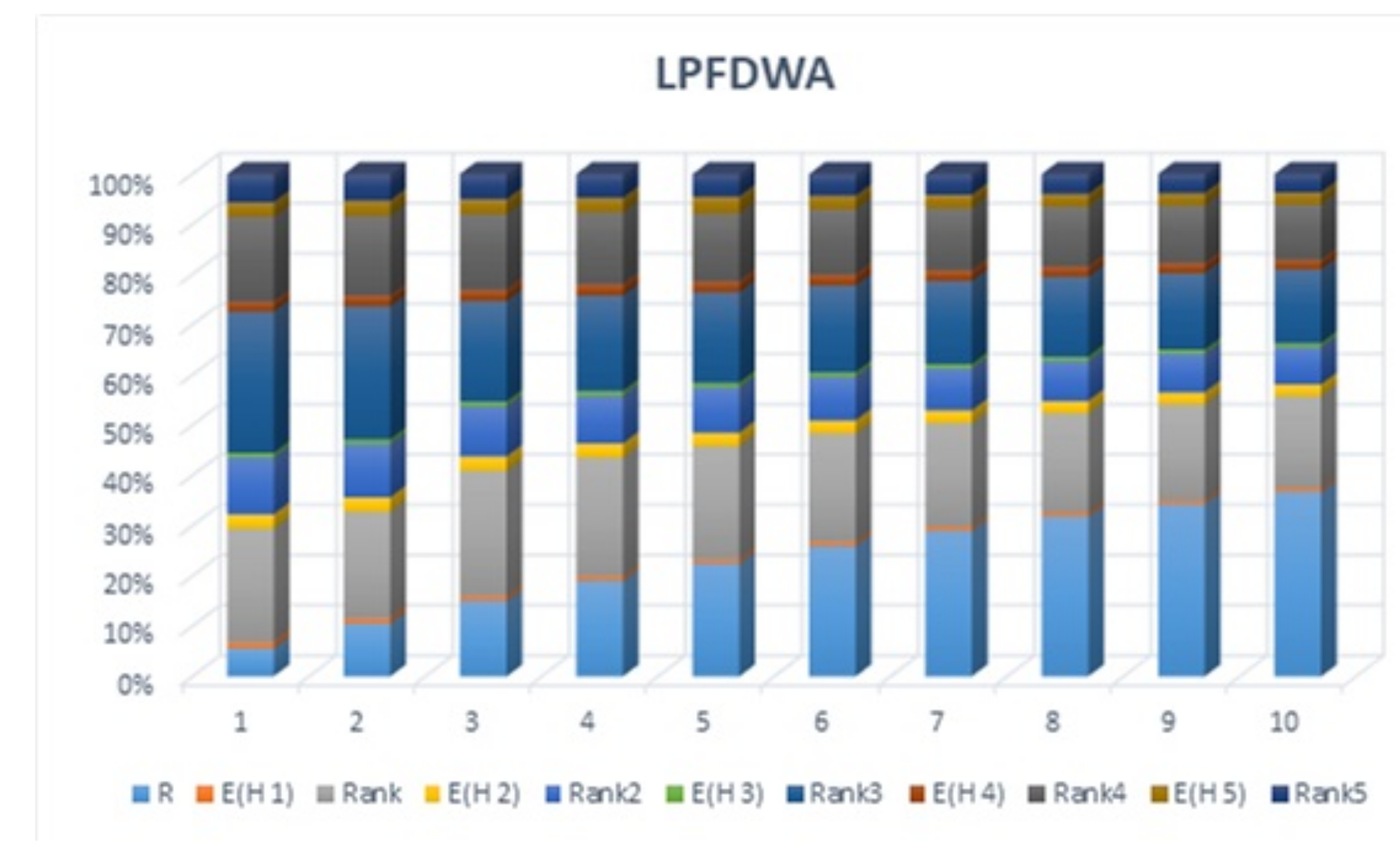
Step 1. Assume that the perimeter $\Re =1,$ and utilize the LPFDWAoperator to compute the total preference values of ${\psi }_g$ of emerging technology enterprises $H_g(g=1,\dots ,5):$

$$\begin{array}{ccc}\hfill {\psi }_1& =& LPFDWA({\psi }_{11},{\psi }_{12},{\psi }_{13},{\psi }_{14})=〈{\acute{s}}_{1.851},{\acute{s}}_{2.790},{\acute{s}}_{2.702}〉,\hfill \\ \hfill {\psi }_2& =& LPFDWA({\psi }_{21},{\psi }_{22},{\psi }_{23},{\psi }_{24})=〈{\acute{s}}_{4.419},{\acute{s}}_{1.463},{\acute{s}}_{1.250}〉,\hfill \\ \hfill {\psi }_3& =& LPFDWA({\psi }_{31},{\psi }_{32},{\psi }_{33},{\psi }_{34})=〈{\acute{s}}_{2.585},{\acute{s}}_{1.538},{\acute{s}}_{2.678}〉,\hfill \\ \hfill {\psi }_4& =& LPFDWA({\psi }_{41},{\psi }_{42},{\psi }_{43},{\psi }_{44})=〈{\acute{s}}_{3.466},{\acute{s}}_{1.621},{\acute{s}}_{2.000}〉,\hfill \\ \hfill {\psi }_5& =& LPFDWA({\psi }_{51},{\psi }_{52},{\psi }_{53},{\psi }_{54})=〈{\acute{s}}_{2.563},{\acute{s}}_{3.468},{\acute{s}}_{1.379}〉.\hfill \end{array}$$

Step 2. Compute the score values using Definition 5, Ē$\left({\psi }_g\right)(g=1,\dots ,5)$ of the all LPFNs as

Ē$\left({\psi }_1\right)=0.2154,$ Ē$\left({\psi }_2\right)=0.5146,$ Ē$\left({\psi }_3\right)=0.1605,$

Ē$\left({\psi }_4\right)=0.343,$ Ē$\left({\psi }_5\right)=0.5168.$

Step 3. According to score values, rank all the emerging technology systems Ē$\left({\psi }_g\right)(g=1,\dots ,5)$ of the LPFNs as

$$H_5>H_2>H_4>H_1>H_{3{.}_{}}$$

Step 4. Thus, Form the

Table 2. Ranking order of influence of the parameters ℜ, using a PFDWA operator.

ℜ	Ē$\left({\mathit{\psi }}_1\right)$	Ē$\left({\mathit{\psi }}_2\right)$	Ē$\left({\mathit{\psi }}_3\right)$	Ē$\left({\mathit{\psi }}_4\right)$	Ē$\left({\mathit{\psi }}_5\right)$	Ranking
1	$0.2154$	$0.5146$	$0.1605$	$0.3430$	$0.5168$	$H_5>H_2>H_4>H_1>H_3$
2	$0.1943$	$0.5441$	$0.1761$	$0.4068$	$0.5747$	$H_5>H_2>H_4>H_1>H_3$
3	$0.1764$	$0.5692$	$0.1874$	$0.4470$	$0.6062$	$H_5>H_2>H_4>H_3>H_1$
4	$0.1698$	$0.5888$	$0.1964$	$0.4716$	$0.6221$	$H_5>H_2>H_4>H_3>H_1$
5	$0.1697$	$0.6014$	$0.2038$	$0.4870$	$0.7423$	$H_5>H_2>H_4>H_3>H_1$
6	$0.1724$	$0.6118$	$0.2100$	$0.4980$	$0.6370$	$H_5>H_2>H_4>H_3>H_1$
7	$0.1757$	$0.6190$	$0.2147$	$0.5060$	$0.6411$	$H_5>H_2>H_4>H_3>H_1$
8	$0.1790$	$0.6252$	$0.2180$	$0.5127$	$0.6440$	$H_5>H_2>H_4>H_3>H_1$
9	$0.1831$	$0.6298$	$0.2220$	$0.5170$	$0.6460$	$H_5>H_2>H_4>H_3>H_1$
10	$0.1862$	$0.6333$	$0.2250$	$0.5212$	$0.6481$	$H_5>H_2>H_4>H_3>H_1$

the most preferable developing technology enterprise is $H_5.$

Ranking results of LPFDWA with average weights are shown in Figure 1.

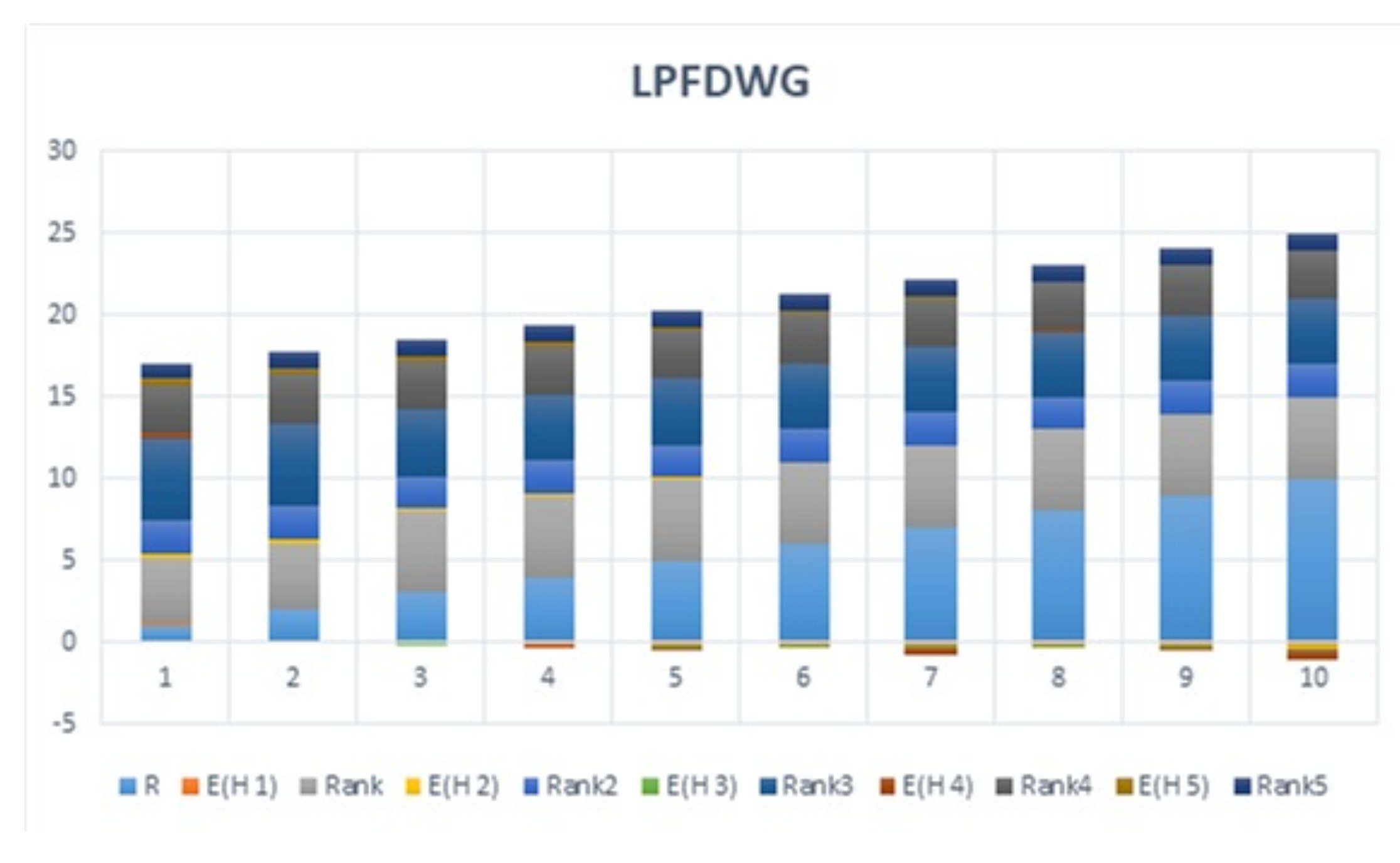
Now, if we use the PFDWG operator, then the problem gives us the following results:

Step 1. Assume the parameter $\Re =1$, and utilize the LPFDWG operator to compute the total preference values of ${\psi }_g$ of emerging technology enterprises $H_g(g=1,\dots ,5).$

$$\begin{array}{ccc}\hfill {\psi }_1& =& LPFDWG({\psi }_{11},{\psi }_{12},{\psi }_{13},{\psi }_{14})=〈{\acute{s}}_{1.578},{\acute{s}}_{2.970},{\acute{s}}_{3.331}〉,\hfill \\ \hfill {\psi }_2& =& LPFDWG({\psi }_{21},{\psi }_{22},{\psi }_{23},{\psi }_{24})=〈{\acute{s}}_{3.821},{\acute{s}}_{1.463},{\acute{s}}_{1.727}〉,\hfill \\ \hfill {\psi }_3& =& LPFDWG({\psi }_{31},{\psi }_{32},{\psi }_{33},{\psi }_{34})=〈{\acute{s}}_{2.222},{\acute{s}}_{1.538},{\acute{s}}_{3.025}〉,\hfill \\ \hfill {\psi }_4& =& LPFDWG({\psi }_{41},{\psi }_{42},{\psi }_{43},{\psi }_{44})=〈{\acute{s}}_{2.579},{\acute{s}}_{1.621},{\acute{s}}_{2.832}〉,\hfill \\ \hfill {\psi }_5& =& LPFDWG({\psi }_{51},{\psi }_{52},{\psi }_{53},{\psi }_{54})=〈{\acute{s}}_{1.449},{\acute{s}}_{3.468},{\acute{s}}_{1.838}〉.\hfill \end{array}$$

Step 2. Compute the score values using Definition 5, Ē$\left({\psi }_g\right)(g=1,2,\dots ,5)$ of the all LPFNs as

Ē$\left({\psi }_1\right)=0.1152,$ Ē$\left({\psi }_2\right)=0.3250,$ Ē$\left({\psi }_3\right)=0.0816,$

Ē$\left({\psi }_4\right)=0.1540,$ Ē$\left({\psi }_5\right)=0.3420.$

Step 3. According to score values, the emerging technology systems Ē$\left({\psi }_g\right)(g=1,2,\dots ,5)$ of the LPFNs ranking are:

$$H_5>H_2>H_4>H_1>H_{3{.}_{}}$$

Step 4. Thus, Form the

Table 3. Ranking order of influence of the parameters ℜ using the PFDWG operator.

ℜ	Ē$\left({\mathit{\psi }}_1\right)$	Ē$\left({\mathit{\psi }}_2\right)$	Ē$\left({\mathit{\psi }}_3\right)$	Ē$\left({\mathit{\psi }}_4\right)$	Ē$\left({\mathit{\psi }}_5\right)$	Ranking
1	$0.1152$	$0.3420$	$0.0816$	$0.1540$	$0.3950$	$H_5>H_2>H_4>H_1>H_3$
2	$0.0114$	$0.3217$	$0.0091$	$0.0777$	$0.3558$	$H_5>H_2>H_4>H_1>H_3$
3	$-$	$0.1668$	$-$	$0.0288$	$0.2711$	$H_5>H_2>H_4>H_3>H_1$
4	$-0.1230$	$0.1101$	$-$	$-$	$0.2370$	$H_5>H_2>H_4>H_3>H_1$
5	$-$	$0.0708$	$-$	$-$	$0.2150$	$H_5>H_2>H_4>H_3>H_1$
6	$-$	$0.0411$	$-$	$0.0372$	$0.1990$	$H_5>H_2>H_4>H_3>H_1$
7	$-$	$0.0199$	$-$	$-$	$0.1870$	$H_5>H_2>H_4>H_3>H_1$
8	$-$	$0.0037$	$-$	$0.0075$	$0.0667$	$H_5>H_2>H_4>H_3>H_1$
9	$-$	$0.0097$	$-$	$-$	$0.1703$	$H_5>H_2>H_4>H_3>H_1$
10	$-$	$-$	$-$	$-$	$0.1647$	$H_5>H_2>H_4>H_3>H_1$

the most preferable developing technology enterprise is $H_2.$

Ranking results of LPFDWG with average weights are shown in Figure 2.

5. Comparative Study

The concept proposed in this article approaches the linguistic picture fuzzy environment, although the existing method [35,37] deals with the picture of fuzzy information and linguistic cubic variables but not in LPFSs. Therefore, our defined operators LPFDWA and LPFDWG operators for the MADM method are more accurate and precise. We compare our method with the Jana et al. [35] and Liu et al. [37]. In

Table 4. Comparison with some other existing approaches.

Method	Ē$\left({\mathit{\psi }}_1\right)$	Ē$\left({\mathit{\psi }}_2\right)$	Ē$\left({\mathit{\psi }}_3\right)$	Ē$\left({\mathit{\psi }}_4\right)$	Ē$\left({\mathit{\psi }}_5\right)$	Ranking
Proposed Method	$0.2154$	$0.5146$	$0.1605$	$0.3430$	$0.5168$	$H_5>H_2>H_4>H_1>H_3$
C. Jana et al.	$0.7293$	$0.8260$	$0.7960$	$0.8112$	$0.8016$	$H_2>H_4>H_5>H_3>H_3$
X. Lu and J. Ye	$0.7620$	$0.7538$	$0.7596$	$0.7507$	$0.7556$	$H_1>H_3>H_5>H_2>H_4$

, we write the comparative results, which show that our introduced methods are ordinary and more workable than other existing methods to control linguistic picture fuzzy MADM problems.

6. Conclusions

Multi-criteria decision-making has continuously been applied to many real-world problems. Many techniques and methods have been proposed by the researchers in recently.

The aim of this manuscript is to present a series of Dombi operators to aggregate the linguistic PF fuzzy information. Some properties like the idempotency, boundedness, and monotonicity of these operators are discussed briefly. The proposed operators are compared with other existing well-known operators, which shows that the proposed operators and their corresponding techniques provide more stability and practicality during the aggregation process. An approach for solving the decision-making problems has been presented by taking different values of ℜ, which makes the proposed operators more flexible and offers various choices to the decision-makers for assessing the decisions.

References

1. Atanassov, K. Intuitionistic fuzzy sets: Theory and applications. In Studies in Fuzziness and Soft Computing; Physica-Verlag: Heidelberg, Germany, 1999; Volume 35. [Google Scholar]
2. Cuong, B.C. Picture Fuzzy Sets—First Results Part 1, Seminar Neuro-Fuzzy Systems with Applications; Technical Report; Institute of Mathematics: Hanoi, Vietnam, 2013. [Google Scholar]
3. Cuong, B.C. Picture fuzzy sets—First Results Part 2, Seminar Neuro-Fuzzy Systems with Applications; Technical Report; Institute of Mathematics: Hanoi, Vietnam, 2013. [Google Scholar]
4. Cuong, B.C. Picture fuzzy sets. J. Comput. Sci. Cybern. 2014, 30, 409–420. [Google Scholar]
5. Cuong, B.C.; Hai, P.V. Some fuzzy logic operators for picture fuzzy sets. In Proceedings of the Seventh International Conference on Knowledge and Systems Engineering, Ho Chi Minh City, Vietnam, 8–10 October 2015; pp. 132–137. [Google Scholar]
6. Cuong, B.C.; Kreinovich, V.; Ngan, R.T. A Classification of Representable T-Norm Operators for Picture Fuzzy Sets. In Proceedings of the 2016 Eighth International Conference on Knowledge and Systems Engineering (KSE), Hanoi, Vietnam, 6–8 October 2016. Departmental Technical Reports (CS) 1047. [Google Scholar]
7. Phong, P.H.; Hieu, D.T.; Ngan, R.T.H.; Them, P.T. Some compositions of picture fuzzy relations. In Proceedings of the 7th National Conference on Fundamental and Applied Information Technology Research, FAIR’7, Thai Nguyen, Vietnam, 19–20 June 2014; pp. 19–20. [Google Scholar]
8. Wei, G.W.; Alsaadi, F.E.; Hayat, T.; Alsaedi, A. Projection models for multiple attribute decision-making with picture fuzzy information. Int. J. Mach. Learn. Cybern. 2018, 9, 713–719. [Google Scholar] [CrossRef]
9. Wei, G.W.; Gao, H. The generalized dice similarity measures for picture fuzzy sets and their applications. Informatica 2018, 29, 1–18. [Google Scholar] [CrossRef]
10. Wei, G.W. Some similarity measures for picture fuzzy sets and their applications. Iran. J. Fuzzy Syst. 2018, 15, 77–89. [Google Scholar]
11. Singh, P. Correlation coefficients for picture fuzzy sets. J. Intell. Fuzzy Syst. 2014, 27, 2857–2868. [Google Scholar]
12. Son, L.H. DPFCM: A novel distributed picture fuzzy clustering method on picture fuzzy sets. Expert Syst. Appl. 2015, 2, 51–66. [Google Scholar] [CrossRef]
13. Thong, P.H.; Son, L.H. A new approach to multi-variables fuzzy forecasting using picture fuzzy clustering and picture fuzzy rules interpolation method. In Proceedings of the 6th International Conference on Knowledge and Systems Engineering, Hanoi, Vietnam, 8–10 October 2015; pp. 679–690. [Google Scholar]
14. Son, L.H. Generalized picture distance measure and applications to picture fuzzy clustering. Appl. Soft Comput. 2016, 46, 284–295. [Google Scholar] [CrossRef]
15. Son, L.H. Measuring analogousness in picture fuzzy sets: From picture distance measures to picture association measures. Fuzzy Optim. Decis. Mak. 2017, 16, 1–20. [Google Scholar] [CrossRef]
16. Son, L.H.; Viet, P.; Hai, P. Picture inference system: A new fuzzy inference system on picture fuzzy set. Appl. Intell. 2017, 46, 652–669. [Google Scholar] [CrossRef]
17. Ashraf, S.; Mahmood, T.; Abdullah, S.; Khan, Q. Different approaches to multi-criteria group decision-making problems for picture fuzzy environment. Bull. Braz. Math. Soc. New Ser. 2019, 50, 373–397. [Google Scholar] [CrossRef]
18. Ashraf, S.; Mahmood, T.; Abdullah, S.; Khan, Q. Picture fuzzy linguistic sets and their applications for multi-attribute group. Nucleus 2018, 55, 66–73. [Google Scholar]
19. Zeng, S.; Asharf, S.; Arif, M.; Abdullah, S. Application of exponential jensen picture fuzzy divergence measure in multi-criteria group decision-making. Mathematics 2019, 7, 191. [Google Scholar] [CrossRef]
20. Khan, M.J.; Kumam, P.; Ashraf, S.; Kumam, W. Generalized Picture Fuzzy Soft Sets and Their Application in Decision Support Systems. Symmetry 2019, 11, 415. [Google Scholar] [CrossRef]
21. Khan, S.; Abdullah, S.; Ashraf, S. Picture fuzzy aggregation information based on Einstein operations and their application in decision-making. Math. Sci. 2019, 1–17. [Google Scholar] [CrossRef]
22. Thong, P.H.; Son, L.H. Picture fuzzy clustering for complex data. Eng. Appl. Artif. Intell. 2016, 56, 121–130. [Google Scholar] [CrossRef]
23. Thong, P.H.; Son, L.H. A novel automatic picture fuzzy clustering method based on particle swarm optimization and picture composite cardinality. Knowl. Based Syst. 2016, 109, 48–60. [Google Scholar] [CrossRef]
24. Khan, S.; Abdullah, S.; Abdullah, L.; Ashraf, S. Logarithmic Aggregation Operators of Picture Fuzzy Numbers for Multi-Attribute Decision Making Problems. Mathematics 2019, 7, 608. [Google Scholar] [CrossRef]
25. Wei, G.W. Picture fuzzy aggregation operators and their application to multiple attribute decision-making. J. Intell. Fuzzy Syst. 2017, 33, 713–724. [Google Scholar] [CrossRef]
26. Peng, X.; Dai, J. Algorithm for picture fuzzy multiple attribute decision-making based on new distance measure. Int. J. Uncertain. Quant. 2017, 7, 177–187. [Google Scholar] [CrossRef]
27. Bo, C.; Zhang, X. New Operations of Picture Fuzzy Relations and Fuzzy Comprehensive Evaluation. Symmetry 2017, 9, 268. [Google Scholar] [CrossRef]
28. Phuong, P.T.M.; Thong, P.H.; Son, L.H. Theoretical analysis of picture fuzzy clustering. J. Comput. Sci. Cybern. 2018, 34, 17–31. [Google Scholar] [CrossRef]
29. Thong, P.H.; Son, L.H.; Fujita, H. Interpolative picture fuzzy rules: A novel forecast method for weather nowcasting. In Proceedings of the 2016 IEEE International Conference on Fuzzy Systems (FUZZ IEEE), Vancouver, BC, Canada, 24–29 July 2016; pp. 86–93. [Google Scholar]
30. Viet, P.V.; Chau, H.T.M.; Son, L.H.; Hai, P.V. Some extensions of membership graphs for picture inference systems, Knowledge and Systems. In Proceedings of the 2015 Seventh International Conference on Knowledge and Systems Engineering (KSE), Ho Chi Minh City, Vietnam, 8–10 October 2015; pp. 192–197. [Google Scholar]
31. Dombi, J. A general class of fuzzy operators, the DeMorgan class of fuzzy operators and fuzziness measures induced by fuzzy operators. Fuzzy Sets Syst. 1982, 8, 149–163. [Google Scholar] [CrossRef]
32. Liu, P.; Liu, J.; Chen, S.M. Some intuitionistic fuzzy Dombi Bonferroni mean operators and their application to multi-attribute group decision-making. J. Oper. Res. Soc. 2018, 69, 1–24. [Google Scholar] [CrossRef]
33. Chen, J.; Ye, J. Some single-valued neutrosophic Dombi weighted aggregation operators for multiple attribute decision-making. Symmetry 2017, 9, 82. [Google Scholar] [CrossRef]
34. Shi, L.; Ye, J. Dombi aggregation operators of neutrosophic cubic sets for multiple attribute decision-making. Algorithms 2018, 11, 29. [Google Scholar]
35. Lu, X.; Ye, J. Dombi aggregation operators of linguistic cubic variables for multiple attribute decision-making. Information 2018, 9, 188. [Google Scholar] [CrossRef]
36. He, X. Typhoon disaster assessment based on Dombi hesitant fuzzy information aggregation operators. Nat. Hazards 2018, 90, 1153–1175. [Google Scholar] [CrossRef]
37. Jana, C.; Senapati, T.; Pal, M.; Yager, R.R. Picture fuzzy Dombi aggregation operators: Application to MADM process. Appl. Soft Comput. 2019, 74, 99–109. [Google Scholar] [CrossRef]
38. Jana, C.; Pal, M.; Wang, J.Q. Bipolar fuzzy Dombi aggregation operators and its application in multiple-attribute decision-making process. J. Ambient. Intell. Humaniz. Comput. 2018, 1–17. [Google Scholar] [CrossRef]
39. Khan, A.A.; Ashraf, S.; Abdullah, S.; Qiyas, M.; Luo, J.; Khan, S.U. Pythagorean fuzzy Dombi aggregation operators and their application in decision support system. Symmetry 2019, 11, 383. [Google Scholar] [CrossRef]
40. Ashraf, S.; Abdullah, S.; Mahmood, T. Spherical fuzzy Dombi aggregation operators and their application in group decision making problems. J. Ambient. Intell. Humaniz. Comput. 2019, 1–19. [Google Scholar] [CrossRef]
41. Cuong, B.C.; Phong, P.H. Max-Min Composition of Linguistic Intuitionistic Fuzzy Relations and Application in Medical Diagnosis. VNU J. Sci. Comput. Sci. Commun. Eng. 2014, 30, 601–968. [Google Scholar]
42. Herrera, F.; Herrera-Viedma, E. Linguistic decision analysis: Steps for solving decision problems under linguistic information. Fuzzy Sets Sys. 2000, 115, 67–82. [Google Scholar] [CrossRef]
43. Zeng, S.; Qiyas, M.; Arif, M.; Mahmood, T. Extended Version of Linguistic Picture Fuzzy TOPSIS Method and Its Applications in Enterprise Resource Planning Systems. Math. Probl. Eng. 2019, 2019, 8594938. [Google Scholar] [CrossRef]
Figure 1. Ranking results of LPFDWA.
Mathematics 07 00764 g001
Figure 2. Ranking results of LPFDWG.
Mathematics 07 00764 g002