Differential Equations Arising from the Generating Function of the (r, β)-Bell Polynomials and Distribution of Zeros of Equations

Abstract

In this paper, we study differential equations arising from the generating function of the $(r,\beta )$-Bell polynomials. We give explicit identities for the $(r,\beta )$-Bell polynomials. Finally, we find the zeros of the $(r,\beta )$-Bell equations with numerical experiments.

1. Introduction

The moments of the Poisson distribution are a well-known connecting tool between Bell numbers and Stirling numbers. As we know, the Bell numbers $B_n$ are those using generating function

$$e^{(e^t-1)}={\displaystyle \sum _{n=0}^{\infty }}{B}_n{\displaystyle \frac{t^n}{n!}}.$$

The Bell polynomials $B_n(\lambda )$ are this formula using the generating function

$$e^{\lambda (e^t-1)}={\displaystyle \sum _{n=0}^{\infty }}{B}_n(\lambda ){\displaystyle \frac{t^n}{n!}},$$

(1)

(see [1,2]).

Observe that

$$B_n(\lambda )={\displaystyle \sum _{i=0}^n}{\lambda }^i{S}_2(n,i),$$

where $S_2(n,i)={\displaystyle \frac{1}{i!}}{\sum }_{l=0}^i{(-1)}^{i-l}\left(\genfrac{}{}{0pt}{}{i}{l}\right)l^n$ denotes the second kind Stirling number.

The generalized Bell polynomials $B_n(x,\lambda )$ are these formula using the generating function:

$${\displaystyle \sum _{n=0}^{\infty }}{B}_n(x,\lambda ){\displaystyle \frac{t^n}{n!}}=e^{xt-\lambda (e^t-t-1)},$$

(see [2]).

In particular, the generalized Bell polynomials $B_n(x,-\lambda )=E_{\lambda }[{(Z+x-\lambda )}^n],\lambda ,x\in \mathbb{R},n\in \mathbb{N},$ where Z is a Poission random variable with parameter $\lambda >0$ (see [1,2,3]). The $(r,\beta )$-Bell polynomials $G_n(x,r,\beta )$ are this formula using the generating function:

$$F(t,x,r,\beta )={\displaystyle \sum _{n=0}^{\infty }}{G}_n(x,r,\beta ){\displaystyle \frac{t^n}{n!}}=e^{rt+(e^{\beta t}-1)\frac{x}{\beta }},$$

(2)

(see [3]), where, $\beta$ and r are real or complex numbers and $(r,\beta )\ne (0,0).$ Note that $B_n(x+r,-x)=G_n(x,r,1)$ and $B_n(x)=G_n(x,0,1)$. The first few examples of $(r,\beta )$-Bell polynomials $G_n(x,r,\beta )$ are

$$\begin{array}{ll}{G}_0(x,r,\beta )=& 1,\\ G_1(x,r,\beta )=& r+x,\\ G_2(x,r,\beta )=& r^2+\beta x+2rx+x^2,\\ G_3(x,r,\beta )=& r^3+{\beta }^{2}x+3\beta rx+3r^{2}x+3\beta x^2+3r{x}^2+x^3,\\ G_4(x,r,\beta )=& r^4+{\beta }^{3}x+4{\beta }^{2}rx+6\beta r^{2}x+4r^{3}x+7{\beta }^2{x}^2+12\beta r{x}^2\\ & +6r^2{x}^2+6\beta x^3+4r{x}^3+x^4,\\ G_5(x,r,\beta )=& r^5+{\beta }^{4}x+5{\beta }^{3}rx+10{\beta }^2{r}^{2}x+10\beta r^{3}x+5r^{4}x+15{\beta }^3{x}^2+35{\beta }^{2}r{x}^2\\ & +30\beta r^2{x}^2+10r^3{x}^2+25{\beta }^2{x}^3+30\beta r{x}^3+10r^2{x}^3+10\beta x^4+5r{x}^4+x^5.\end{array}$$

From (1) and (2), we see that

$$\begin{array}{ll}{\displaystyle \sum _{n=0}^{\infty }}{G}_n(x,r,\beta ){\displaystyle \frac{t^n}{n!}}& =e^{(e^{\beta t}-1)\frac{x}{\beta }}{e}^{rt}\\ & =\left({\displaystyle \sum _{k=0}^{\infty }}{B}_k(x/\beta ){\beta }^k{\displaystyle \frac{t^k}{k!}}\right)\left({\displaystyle \sum _{m=0}^{\infty }}{r}^m{\displaystyle \frac{t^m}{m!}}\right)\\ & ={\displaystyle \sum _{n=0}^{\infty }}\left({\displaystyle \sum _{k=0}^n}\left(\genfrac{}{}{0pt}{}{n}{k}\right)B_k(x/\beta ){\beta }^k{r}^{n-k}\right){\displaystyle \frac{t^n}{n!}}.\end{array}$$

(3)

Compare the coefficients in Formula (3). We can get

$$G_n(x,r,\beta )={\displaystyle \sum _{k=0}^n}\left(\genfrac{}{}{0pt}{}{n}{k}\right){\beta }^k{B}_k(x/\beta )r^{n-k},(n\ge 0).$$

Similarly we also have

$$G_n(x+y,r,\beta )={\displaystyle \sum _{k=0}^n}\left(\genfrac{}{}{0pt}{}{n}{k}\right)G_k(x,r,\beta )B_{n-k}(y/\beta ){\beta }^{n-l}.$$

Recently, many mathematicians have studied the differential equations arising from the generating functions of special polynomials (see [4,5,6,7,8]). Inspired by their work, we give a differential equations by generation of $(r,\beta )$-Bell polynomials $G_n(x,r,\beta )$ as follows. Let D denote differentiation with respect to t, $D^2$ denote differentiation twice with respect to t, and so on; that is, for positive integer N,

$$D^{N}F={\left({\displaystyle \frac{\partial }{\partial t}}\right)}^{N}F(t,x,r,\beta ).$$

We find differential equations with coefficients $a_i(N,x,r,\beta )$, which are satisfied by

$${\left({\displaystyle \frac{\partial }{\partial t}}\right)}^{N}F(t,x,r,\beta )-a_0(N,x,r,\beta )F(t,x,r,\beta )-\cdots -a_N(N,x,r,\beta )e^{\beta tN}F(t,x,r,\beta )=0.$$

Using the coefficients of this differential equation, we give explicit identities for the $(r,\beta )$-Bell polynomials. In addition, we investigate the zeros of the $(r,\beta )$-Bell equations with numerical methods. Finally, we observe an interesting phenomena of ‘scattering’ of the zeros of $(r,\beta )$-Bell equations. Conjectures are also presented through numerical experiments.

2. Differential Equations Related to $(\mathit{R},\mathit{\beta })$-Bell Polynomials

Differential equations arising from the generating functions of special polynomials are studied by many authors to give explicit identities for special polynomials (see [4,5,6,7,8]). In this section, we study differential equations arising from the generating functions of $(r,\beta )$-Bell polynomials.

Let

$$F=F(t,x,r,\beta )={\displaystyle \sum _{n=0}^{\infty }}{G}_n(x,r,\beta ){\displaystyle \frac{t^n}{n!}}=e^{rt+(e^{\beta t}-1)\frac{x}{\beta }},x,r,\beta \in \mathbb{C}.$$

(4)

Then, by (4), we have

$$\begin{array}{ll}DF={\displaystyle \frac{\partial }{\partial t}}F(t,x,r,\beta )& ={\displaystyle \frac{\partial }{\partial t}}\left(e^{rt+(e^{\beta t}-1)\frac{x}{\beta }}\right)\\ & =e^{rt+(e^{\beta t}-1)\frac{x}{\beta }}(r+x{e}^{\beta t})\\ & =r{e}^{rt+(e^{\beta t}-1)\frac{x}{\beta }}+x{e}^{(r+\beta )t+(e^{\beta t}-1)\frac{x}{\beta }}\\ & =rF(t,x,r,\beta )+xF(t,x,r+\beta ,\beta ),\end{array}$$

(5)

$$\begin{array}{ll}{D}^{2}F& =rDF(t,x,r,\beta )+xDF(t,x,r+\beta ,\beta )\\ & =r^{2}F(t,x,r,\beta )+x(2r+\beta )F(t,x,r+\beta ,\beta )+x^{2}F(t,x,r+2\beta ,\beta ),\end{array}$$

(6)

and

$$\begin{array}{ll}{D}^{3}F& =r^{2}DF(t,x,r,\beta )+x(2r+\beta )DF(t,x,r+\beta ,\beta )+x^{2}DF(t,x,r+2\beta ,\beta )\\ & =r^{3}F(t,x,r,\beta )+x\left(r^2+(2r+\beta )(r+\beta )\right)F(t,x,r+\beta ,\beta )\\ & +x^2(3r+3\beta )F(t,x,r+2\beta ,\beta )+x^{3}F(t,x,r+3\beta ,\beta ).\end{array}$$

We prove this process by induction. Suppose that

$$D^{N}F={\displaystyle \sum _{i=0}^N}{a}_i(N,x,r,\beta )F(t,x,r+i\beta ,\beta ),(N=0,1,2,\dots ).$$

(7)

is true for N. From (7), we get

$$\begin{array}{ll}{D}^{N+1}F& ={\displaystyle \sum _{i=0}^N}{a}_i(N,x,r,\beta )DF(t,x,r+i\beta ,\beta )\\ & ={\displaystyle \sum _{i=0}^N}{a}_i(N,x,r,\beta )\left\{(r+i\beta )F(t,x,r+i\beta ,\beta )+xF(t,x,r+(i+1)\beta ,\beta )\right\}\\ & ={\displaystyle \sum _{i=0}^N}{a}_i(N,x,r,\beta )(r+i\beta )F(t,x,r+i\beta ,\beta )\\ & +x{\displaystyle \sum _{i=0}^N}{a}_i(N,x,r,\beta )F(t,x,r+(i+1)\beta ,\beta )\\ & ={\displaystyle \sum _{i=0}^N}(r+i\beta )a_i(N,x,r,\beta )F(t,x,r+i\beta ,\beta )\\ & +x{\displaystyle \sum _{i=1}^{N+1}}{a}_{i-1}(N,x,r,\beta )F(t,x,r+i\beta ,\beta ).\end{array}$$

(8)

From (8), we get

$$D^{N+1}F={\displaystyle \sum _{i=0}^{N+1}}{a}_i(N+1,x,r,\beta )F(t,x,r+i\beta ,\beta ).$$

(9)

We prove that

$$D^{k+1}F={\displaystyle \sum _{i=0}^{k+1}}{a}_i(k+1,x,r,\beta )F(t,x,r+i\beta ,\beta ).$$

If we compare the coefficients on both sides of (8) and (9), then we get

$$a_0(N+1,x,r,\beta )=r{a}_0(N,x,r,\beta ),a_{N+1}(N+1,x,r,\beta )=x{a}_N(N,x,r,\beta ),$$

(10)

and

$$a_i(N+1,x,r,\beta )=(r+i\beta )a_{i-1}(N,x,r,\beta )+x{a}_{i-1}(N,x,r,\beta ),(1\le i\le N).$$

(11)

In addition, we get

$$F(t,x,r,\beta )=a_0(0,x,r,\beta )F(t,x,r,\beta ).$$

(12)

Now, by (10), (11) and (12), we can obtain the coefficients $a_i{(j,x,r,\beta )}_{0\le i,j\le N+1}$ as follows. By (12), we get

$$a_0(0,x,r,\beta )=1.$$

(13)

It is not difficult to show that

$$\begin{array}{l}rF(t,x,r,\beta )+xF(t,x,r+\beta ,\beta )\\ =DF(t,x,r,\beta )\\ ={\displaystyle \sum _{i=0}^1}{a}_i(1,x,r,\beta )F(t,x,r+\beta ,\beta )\\ =a_0(1,x,r,\beta )F(t,x,r,\beta )+a_1(1,x,r,\beta )F(t,x,r+\beta ,\beta ).\end{array}$$

(14)

Thus, by (14), we also get

$$a_0(1,x,r,\beta )=r,a_1(1,x,r,\beta )=x.$$

(15)

From (10), we have that

$$a_0(N+1,x,r,\beta )=r{a}_0(N,x,r,\beta )=\cdots =r^N{a}_0(1,x,r,\beta )=r^{N+1},$$

(16)

and

$$a_{N+1}(N+1,x,r,\beta )=x{a}_N(N,x,r,\beta )=\cdots =x^N{a}_1(1,x,r,\beta )=x^{N+1}.$$

(17)

For $i=1,2,3$ in (11), we have

$$a_1(N+1,x,r,\beta )=x{\displaystyle \sum _{k=0}^N}{(r+\beta )}^k{a}_0(N-k,x,r,\beta ),$$

(18)

$$a_2(N+1,x,r,\beta )=x{\displaystyle \sum _{k=0}^{N-1}}{(r+2\beta )}^k{a}_1(N-k,x,r,\beta ),$$

(19)

and

$$a_3(N+1,x,r,\beta )=x{\displaystyle \sum _{k=0}^{N-2}}{(r+3\beta )}^k{a}_2(N-k,x,r,\beta ).$$

(20)

By induction on i, we can easily prove that, for $1\le i\le N,$

$$a_i(N+1,x,r,\beta )=x{\displaystyle \sum _{k=0}^{N-i+1}}{(r+i\beta )}^k{a}_{i-1}(N-k,x,r,\beta ).$$

(21)

Here, we note that the matrix $a_i{(j,x,r,\beta )}_{0\le i,j\le N+1}$ is given by

$$\left(\begin{array}{cccccc}1& r& r^2& r^3& \cdots & r^{N+1}\\ 0& x& x(2r+\beta )& x(3r^2+3r\beta +{\beta }^2)& \cdots & ·\\ 0& 0& x^2& x^2(3r+3\beta )& \cdots & ·\\ 0& 0& 0& x^3& \cdots & ·\\ ⋮& ⋮& ⋮& ⋮& \ddots & ⋮\\ 0& 0& 0& 0& \cdots & x^{N+1}\end{array}\right)$$

Now, we give explicit expressions for $a_i(N+1,x,r,\beta )$. By (18), (19), and (20), we get

$$\begin{array}{ll}{a}_1(N+1,x,r,\beta )=& x{\displaystyle \sum _{k_1=0}^N}{(r+\beta )}^{k_1}{a}_0(N-k_1,x,r,\beta )\\ & ={\displaystyle \sum _{k_1=0}^N}{(r+\beta )}^{k_1}{r}^{N-k_1},\end{array}$$

$$\begin{array}{ll}{a}_2(N+1,x,r,\beta )=& x{\displaystyle \sum _{k_2=0}^{N-1}}{(r+2\beta )}^{k_2}{a}_1(N-k_2,x,r,\beta )\\ & =x^2{\displaystyle \sum _{k_2=0}^{N-1}}{\displaystyle \sum _{k_1=0}^{N-1-k_2}}{(r+\beta )}^{k_1}{(r+2\beta )}^{k_2}{r}^{N-k_2-k_1-1},\end{array}$$

and

$$\begin{array}{l}{a}_3(N+1,x,r,\beta )\\ =x{\displaystyle \sum _{k_3=0}^{N-2}}{(r+3\beta )}^{k_3}{a}_2(N-k_3,x,r,\beta )\\ =x^3{\displaystyle \sum _{k_3=0}^{N-2}}{\displaystyle \sum _{k_2=0}^{N-2-k_3}}{\displaystyle \sum _{k_1=0}^{N-2-k_3-k_2}}{(r+3\beta )}^{k_3}{(r+2\beta )}^{k_2}{(r+\beta )}^{k_1}{r}^{N-k_3-k_2-k_1-2}.\end{array}$$

By induction on i, we have

$$\begin{array}{l}{a}_i(N+1,x,r,\beta )\\ =x^i{\displaystyle \sum _{k_i=0}^{N-i+1}}{\displaystyle \sum _{k_{i-1}=0}^{N-i+1-k_i}}\cdots {\displaystyle \sum _{k_1=0}^{N-i+1-k_i-\cdots -k_2}}\left({\displaystyle \prod _{l=1}^i}{(r+l\beta )}^{k_l}\right)r^{N-i+1-{\sum }_{l=1}^i{k}_l}.\end{array}$$

(22)

Finally, by (22), we can derive a differential equations with coefficients $a_i(N,x,r,\beta )$, which is satisfied by

$${\left({\displaystyle \frac{\partial }{\partial t}}\right)}^{N}F(t,x,r,\beta )-a_0(N,x,r,\beta )F(t,x,r,\beta )-\cdots -a_N(N,x,r,\beta )e^{\beta tN}F(t,x,r,\beta )=0.$$

Theorem 1.

For same as below $N=0,1,2,\dots ,$ the differential equation

$$D^{N}F={\displaystyle \sum _{i=0}^N}{a}_i(N,x,r,\beta )e^{i\beta t}F(t,x,r,\beta )$$

has a solution

$$F=F(t,x,r,\beta )=e^{rt+(e^{\beta t}-1)\frac{x}{\beta }},$$

where

$$\begin{array}{l}{a}_0(N,x,r,\beta )=r^N,\\ a_N(N,x,r,\beta )=x^N,\\ a_i(N,x,r,\beta )=x^i{\displaystyle \sum _{k_i=0}^{N-i}}{\displaystyle \sum _{k_{i-1}=0}^{N-i-k_i}}\cdots {\displaystyle \sum _{k_1=0}^{N-i-k_i-\cdots -k_2}}\left({\displaystyle \prod _{l=1}^i}{(r+l\beta )}^{k_l}\right)r^{N-i-{\sum }_{l=1}^i{k}_l},\\ (1\le i\le N).\end{array}$$

From (4), we have this

$$D^{N}F={\left({\displaystyle \frac{\partial }{\partial t}}\right)}^{N}F(t,x,r,\beta )={\displaystyle \sum _{k=0}^{\infty }}{G}_{k+N}(x,r,\beta ){\displaystyle \frac{t^k}{k!}}.$$

(23)

By using Theorem 1 and (23), we can get this equation:

$$\begin{array}{ll}{\displaystyle \sum _{k=0}^{\infty }}{G}_{k+N}(x,r,\beta ){\displaystyle \frac{t^k}{k!}}& =D^{N}F\\ & =\left({\displaystyle \sum _{i=0}^N}{a}_i(N,x,r,\beta )e^{i\beta t}\right)F(t,x,r,\beta )\\ & ={\displaystyle \sum _{i=0}^N}{a}_i(N,x,r,\beta )\left({\displaystyle \sum _{l=0}^{\infty }}{(i\beta )}^l{\displaystyle \frac{t^l}{l!}}\right)\left({\displaystyle \sum _{m=0}^{\infty }}{G}_m(x,r,\beta ){\displaystyle \frac{t^m}{m!}}\right)\\ & ={\displaystyle \sum _{i=0}^N}{a}_i(N,x,r,\beta )\left({\displaystyle \sum _{k=0}^{\infty }}{\displaystyle \sum _{m=0}^k}\left(\genfrac{}{}{0pt}{}{k}{m}\right){(i\beta )}^{k-m}{G}_m(x,r,\beta ){\displaystyle \frac{t^k}{k!}}\right)\\ & ={\displaystyle \sum _{k=0}^{\infty }}\left({\displaystyle \sum _{i=0}^N}{\displaystyle \sum _{m=0}^k}\left(\genfrac{}{}{0pt}{}{k}{m}\right){(i\beta )}^{k-m}{a}_i(N,x,r,\beta )G_m(x,r,\beta )\right){\displaystyle \frac{t^k}{k!}}.\end{array}$$

(24)

Compare coefficients in (24). We get the below theorem.

Theorem 2.

For $k,N=0,1,2,\dots ,$ we have

$$G_{k+N}(x,r,\beta )={\displaystyle \sum _{i=0}^N}{\displaystyle \sum _{m=0}^k}\left(\genfrac{}{}{0pt}{}{k}{m}\right)i^{k-m}{\beta }^{k-m}{a}_i(N,x,r,\beta )G_m(x,r,\beta ),$$

(25)

where

$$\begin{array}{l}{a}_0(N,x,r,\beta )=r^N,\\ a_N(N,x,r,\beta )=x^N,\\ a_i(N,x,r,\beta )=x^i{\displaystyle \sum _{k_i=0}^{N-i}}{\displaystyle \sum _{k_{i-1}=0}^{N-i-k_i}}\cdots {\displaystyle \sum _{k_1=0}^{N-i-k_i-\cdots -k_2}}\left({\displaystyle \prod _{l=1}^i}{(r+l\beta )}^{k_l}\right)r^{N-i-{\sum }_{l=1}^i{k}_l},\\ (1\le i\le N).\end{array}$$

By using the coefficients of this differential equation, we give explicit identities for the $(r,\beta )$-Bell polynomials. That is, in (25) if $k=0$, we have corollary.

Corollary 1.

For $N=0,1,2,\dots ,$ we have

$$G_N(x,r,\beta )={\displaystyle \sum _{i=0}^N}{a}_i(N,x,r,\beta ).$$

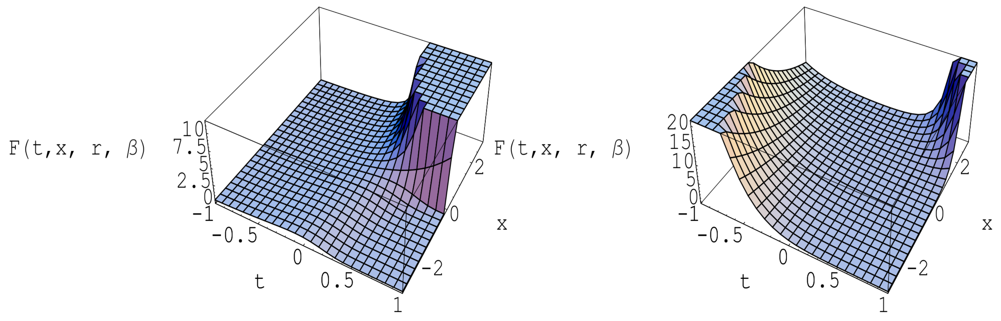
For $N=0,1,2,\dots ,$ it follows that equation

$$D^{N}F-{\displaystyle \sum _{i=0}^N}{a}_i(N,x,r,\beta )e^{i\beta t}F(t,x,r,\beta )=0$$

has a solution

$$F=F(t,x,r,\beta )=e^{rt+(e^{\beta t}-1)\frac{x}{\beta }}.$$

In Figure 1, we have a sketch of the surface about the solution F of this differential equation. On the left of Figure 1, we give $-3\le x\le 3,-1\le t\le 1,$ and $r=2,\beta =5$. On the right of Figure 1, we give $-3\le x\le 3,-1\le t\le 1,$ and $r=-3,\beta =2$.

Making N-times derivative for (4) with respect to t, we obtain

$${\left({\displaystyle \frac{\partial }{\partial t}}\right)}^{N}F(t,x,r,\beta )={\left({\displaystyle \frac{\partial }{\partial t}}\right)}^N{e}^{rt+(e^{\beta t}-1)\frac{x}{\beta }}={\displaystyle \sum _{m=0}^{\infty }}{G}_{m+N}(x,r,\beta ){\displaystyle \frac{t^m}{m!}}.$$

(26)

By multiplying the exponential series $e^{xt}={\sum }_{m=0}^{\infty }{x}^m{\displaystyle \frac{t^m}{m!}}$ in both sides of (26) and Cauchy product, we derive

$$\begin{array}{ll}{e}^{-nt}{\left({\displaystyle \frac{\partial }{\partial t}}\right)}^{N}F(t,x,r,\beta )& =\left({\displaystyle \sum _{m=0}^{\infty }}{(-n)}^m{\displaystyle \frac{t^m}{m!}}\right)\left({\displaystyle \sum _{m=0}^{\infty }}{G}_{m+N}(x,r,\beta ){\displaystyle \frac{t^m}{m!}}\right)\\ & ={\displaystyle \sum _{m=0}^{\infty }}\left({\displaystyle \sum _{k=0}^m}\left(\genfrac{}{}{0pt}{}{m}{k}\right){(-n)}^{m-k}{G}_{N+k}(x,r,\beta )\right){\displaystyle \frac{t^m}{m!}}.\end{array}$$

(27)

By using the Leibniz rule and inverse relation, we obtain

$$\begin{array}{ll}{e}^{-nt}{\left({\displaystyle \frac{\partial }{\partial t}}\right)}^{N}F(t,x,y)& ={\displaystyle \sum _{k=0}^N}\left(\genfrac{}{}{0pt}{}{N}{k}\right)n^{N-k}{\left({\displaystyle \frac{\partial }{\partial t}}\right)}^k\left(e^{-nt}F(t,x,r,\beta )\right)\\ & ={\displaystyle \sum _{m=0}^{\infty }}\left({\displaystyle \sum _{k=0}^N}\left(\genfrac{}{}{0pt}{}{N}{k}\right)n^{N-k}{G}_{m+k}(x-n,r,\beta )\right){\displaystyle \frac{t^m}{m!}}.\end{array}$$

(28)

So using (27) and (28), and using the coefficients of ${\displaystyle \frac{t^m}{m!}}$ gives the below theorem.

Theorem 3.

Let $m,n,N$ be nonnegative integers. Then

$${\displaystyle \sum _{k=0}^m}\left(\genfrac{}{}{0pt}{}{m}{k}\right){(-n)}^{m-k}{G}_{N+k}(x,r,\beta )={\displaystyle \sum _{k=0}^N}\left(\genfrac{}{}{0pt}{}{N}{k}\right)n^{N-k}{G}_{m+k}(x-n,r,\beta ).$$

(29)

When we give $m=0$ in (29), then we get corollary.

Corollary 2.

For $N=0,1,2,\dots ,$ we have

$$G_N(x,r,\beta )={\displaystyle \sum _{k=0}^N}\left(\genfrac{}{}{0pt}{}{N}{k}\right)n^{N-k}{G}_k(x-n,r,\beta ).$$

3. Distribution of Zeros of the $(\mathit{R},\mathit{\beta })$-Bell Equations

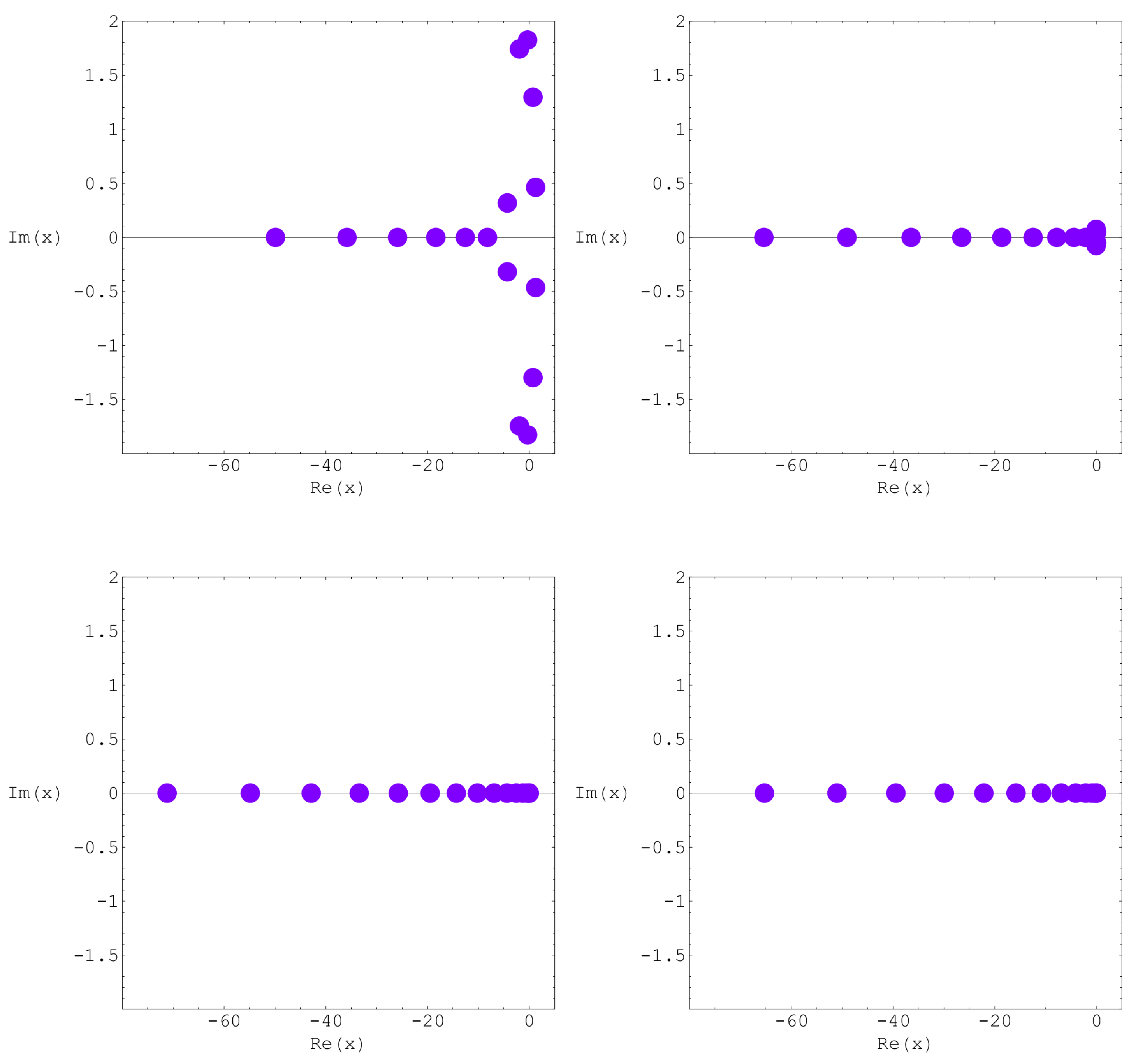
This section aims to demonstrate the benefit of using numerical investigation to support theoretical prediction and to discover new interesting patterns of the zeros of the $(r,\beta )$-Bell equations $G_n(x,r,\beta )=0$. We investigate the zeros of the $(r,\beta )$-Bell equations $G_n(x,r,\beta )=0$ with numerical experiments. We plot the zeros of the $B_n(x,\lambda )=0$ for $n=16,r=-5,-3,3,5,\beta =2,3$ and $x\in \mathbb{C}$ (Figure 2).

In top-left of Figure 2, we choose $n=16$ and $r=-5$, $\beta =2$. In top-right of Figure 2, we choose $n=16$ and $r=-3$, $\beta =3$. In bottom-left of Figure 2, we choose $n=16$ and $r=3,\beta =2$. In bottom-right of Figure 2, we choose $n=16$ and $r=5,\beta =3$.

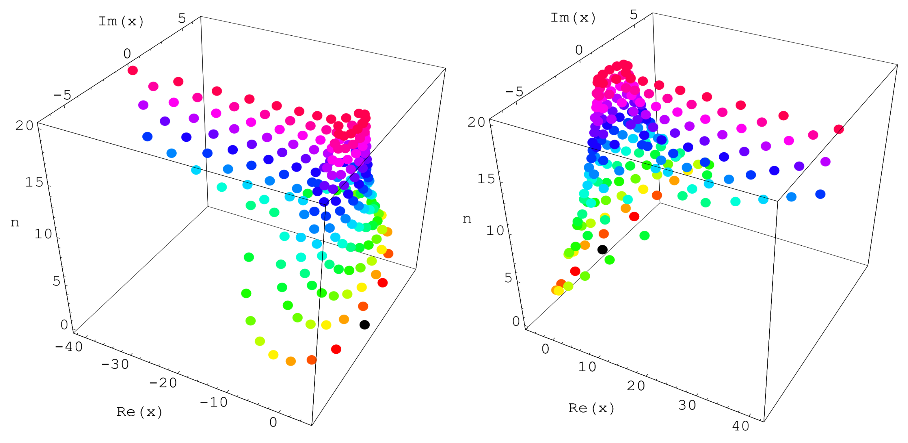
Prove that $G_n(x,r,\beta ),x\in \mathbb{C}$, has $Im(x)=0$ reflection symmetry analytic complex functions (see Figure 3). Stacks of zeros of the $(r,\beta )$-Bell equations $G_n(x,r,\beta )=0$ for $1\le n\le 20$ from a 3-D structure are presented (Figure 3).

On the left of Figure 3, we choose $r=-5$ and $\beta =2$. On the right of Figure 3, we choose $r=5$ and $\beta =2$. In Figure 3, the same color has the same degree n of $(r,\beta )$-Bell polynomials $G_n(x,r,\beta )$. For example, if $n=20$, zeros of the $(r,\beta )$-Bell equations $G_n(x,r,\beta )=0$ is red.

Our numerical results for approximate solutions of real zeros of the $(r,\beta )$-Bell equations $G_n(x,r,\beta )=0$ are displayed (

Table 1. Numbers of real and complex zeros of $G_n(x,r,\beta )=0$.

Degree n	$\mathit{r}=-5,\mathit{\beta }=2$		$\mathit{r}=5,\mathit{\beta }=2$
	Real Zeros	Complex Zeros	Real Zeros	Xomplex Zeros
1	1	0	1	0
2	0	2	2	0
3	1	2	3	0
4	0	4	4	0
5	1	4	5	0
6	0	6	6	0
7	1	6	7	0
8	0	8	8	0
9	1	8	9	0
10	2	8	10	0

and

Table 2. Approximate solutions of $G_n(x,r,\beta )=0,x\in \mathbb{R}$.

Degree n	x
1	−5.000
2	−9.317,    −2.683
3	−13.72,    −5.68,    −1.605
4	−18.21,    −9.01,    −3.77,    −1.010
5	−22.8,    −12.6,    −6.4,    −2.61,    −0.655
6	−27.4,    −16.3,    −9.3,    −4.7,    −1.85,    −0.434
7	−32.0,    −20.0,    −12.0,    −7.1,    −3.5,    −1.34,    −0.291

).

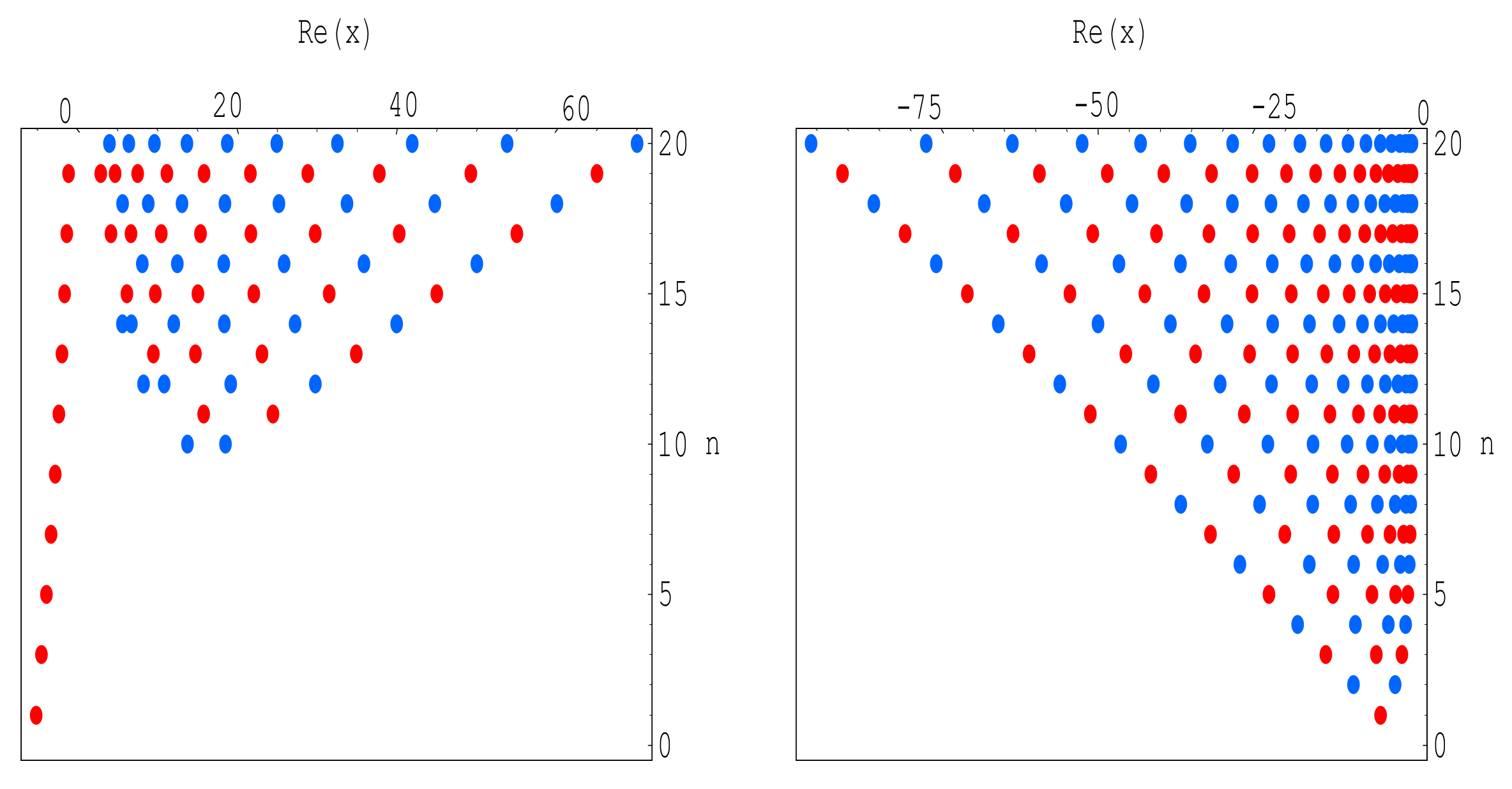
Plot of real zeros of $G_n(x,r,\beta )=0$ for $1\le n\le 20$ structure are presented (Figure 4).

In Figure 4 (left), we choose $r=5$ and $\beta =-2$. In Figure 4 (right), we choose $r=5$ and $\beta =2$. In Figure 4, the same color has the same degree n of $(r,\beta )$-Bell polynomials $G_n(x,r,\beta )$. For example, if $n=20$, real zeros of the $(r,\beta )$-Bell equations $G_n(x,r,\beta )=0$ is blue.

Next, we calculated an approximate solution satisfying $G_n(x,r,\beta )=0,r=5,\beta =2,x\in \mathbb{R}$. The results are given in Table 2.

4. Conclusions

We constructed differential equations arising from the generating function of the $(r,\beta )$-Bell polynomials. This study obtained the some explicit identities for $(r,\beta )$-Bell polynomials $G_n(x,r,\beta )$ using the coefficients of this differential equation. The distribution and symmetry of the roots of the $(r,\beta )$-Bell equations $G_n(x,r,\beta )=0$ were investigated. We investigated the symmetry of the zeros of the $(r,\beta )$-Bell equations $G_n(x,r,\beta )=0$ for various variables r and $\beta$, but, unfortunately, we could not find a regular pattern. We make the following series of conjectures with numerical experiments:

Let us use the following notations. $R_{G_n(x,r,\beta )}$ denotes the number of real zeros of $G_n(x,r,\beta )=0$ lying on the real plane $Im(x)=0$ and $C_{G_n(x,r,\beta )}$ denotes the number of complex zeros of $G_n(x,r,\beta )=0$. Since n is the degree of the polynomial $G_n(x,r,\beta )$, we have $R_{G_n(x,r,\beta )}=n-C_{G_n(x,r,\beta )}$ (see Table 1).

We can see a good regular pattern of the complex roots of the $(r,\beta )$-Bell equations $G_n(x,r,\beta )=0$ for $r>0$ and $\beta >0$. Therefore, the following conjecture is possible.

Conjecture 1.

For $r>0$ and $\beta >0$, prove or disprove that

$$C_{H_n(x,y)}=0.$$

As a result of investigating more $r>0$ and $\beta >0$ variables, it is still unknown whether the conjecture 1 is true or false for all variables $r>0$ and $\beta >0$ (see Figure 1 and Table 1).

We observe that solutions of $(r,\beta )$-Bell equations $G_n(x,r,\beta )=0$ has $Im(x)=0$, reflecting symmetry analytic complex functions. It is expected that solutions of $(r,\beta )$-Bell equations $G_n(x,r,\beta )=0$, has not $Re(x)=a$ reflection symmetry for $a\in \mathbb{R}$ (see Figure 2, Figure 3 and Figure 4).

Conjecture 2.

Prove or disprove that solutions of $(r,\beta )$-Bell equations $G_n(x,r,\beta )=0$, has not $Re(x)=a$ reflection symmetry for $a\in \mathbb{R}$.

Finally, how many zeros do $G_n(x,r,\beta )=0$ have? We are not able to decide if $G_n(x,r,\beta )=0$ has n distinct solutions (see Table 1 and Table 2). We would like to know the number of complex zeros $C_{G_n(x,r,\beta )}$ of $G_n(x,r,\beta )=0,Im(x)\ne 0.$

Conjecture 3.

Prove or disprove that $G_n(x,r,\beta )=0$ has n distinct solutions.

As a result of investigating more n variables, it is still unknown whether the conjecture is true or false for all variables n (see Table 1 and Table 2). We expect that research in these directions will make a new approach using the numerical method related to the research of the $(r,\beta )$-Bell numbers and polynomials which appear in mathematics, applied mathematics, statistics, and mathematical physics. The reader may refer to [5,6,7,8,9,10] for the details.