Iterative Methods for Solving a System of Linear Equations in a Bipolar Fuzzy Environment

Abstract

We develop the solution procedures to solve the bipolar fuzzy linear system of equations (BFLSEs) with some iterative methods namely Richardson method, extrapolated Richardson (ER) method, Jacobi method, Jacobi over-relaxation (JOR) method, Gauss–Seidel (GS) method, extrapolated Gauss-Seidel (EGS) method and successive over-relaxation (SOR) method. Moreover, we discuss the properties of convergence of these iterative methods. By showing the validity of these methods, an example having exact solution is described. The numerical computation shows that the SOR method with $\omega =1.25$ is more accurate as compared to the other iterative methods.

1. Introduction

Certain problems existing in the field of economics, social sciences and engineering involve vagueness, imprecision and uncertainty. To overcome this difficulty, Zadeh [1] introduce the idea of fuzzy set in 1965. This development can be used to extend the crisp mathematical idea into fuzzy information. Formally, the basic arithmetic operations were constructed by Dubois and Prade [2,3], Tanaka and Mizumoto [4,5] and Nahmias [6], and they also discussed the fuzzy numbers methods. The parametric form of fuzzy numbers and perception of fuzzy calculus were proposed by Voxman and Goetschel [7]. Further, they extended their work to imbed the set of parametric fuzzy numbers into a topological vector space. The notion of trapezoidal fuzzy numbers was preceded by Moghadam et al. [8]. Further, related to their presented work, Wu and Ma [9], Puri and Ralescu [10] analyzed the several other useful concepts in literature. Linear system plays a significant role in the field of engineering and sciences. In the vast majority of problems, we usually work with approximate data. In several applications, few parameters are expressed as fuzzy and more general bipolar fuzzy instead of the crisp number. It is extremely essential to propose the numerical techniques that would suitably treat bipolar fuzzy linear system of equations (BFLSEs) and solve them. There is a vast literature on the solution of the fuzzy system of linear equations (FSLEs) with real crisp coefficient entries and vector on the right-hand side (RHS) is parametric fuzzy numbers (PFNs) arises in many domains of technology and engineering sciences such as telecommunications, statistics, economics, social sciences, image processing and even in physics. In [11,12], one of the most important application is presented by using the arithmetics of fuzzy numbers, applying them on linear systems with their parameters.

Friedman [13] studied the general solution to the FSLEs with crisp coefficient entries of the matrix and the RHS column vector function is the PFNs. Friedman used the embedding technique and replaced $n\times n$ original FSLEs to the extended $2n\times 2n$ FSLEs. Many authors studied FSLEs. There are several reported studies through which many authors attract our attention to solve the FSLEs numerically. Various procedures for solving fuzzy systems would be used by many authors. These methods depend on the fuzzy variables, fuzzy matrix and fuzzy vectors to the right hand side (RHS) of the system, etc. Allahviranloo [14,15] developed the Jacobi, GS and SOR iterative scheme to solve the FSLEs in numerical way. Dehghan et al. [16] considered the solution existence of the linear system in the fuzzy environment provided that real crisp coefficient entries are strictly and diagonally dominant having positive diagonal elements and then various iterative methods applied. Ezzati [17] introduced the new method to solve the FSLEs to use the embedding technique and replaced the original $n\times n$ FSLEs to the extended $2n\times 2n$ crisp FSLEs. Moreover, Muzziolia et al. [18] introduced fuzzy system of linear equations in the form of $A_{1}x+b_1=A_{2}x+b_2$ with fuzzy coefficients $A_1$ and $A_2$ are $n\times n$ matrices and $b_1,b_2$ fuzzy number vectors. Allahviranloo et al. [19,20,21] introduce some numerical techniques for solving FSLEs. Abbasbandy et al. [22] introduced the steepest descent method to solve FSLEs. The numerical technique for solving the linear system in a fuzzy and fully fuzzy environment was studied by Ineirat [23]. For the most part, FSLEs is dealing under two fundamental headings. One is square and the other is rectangular frames. Most work in the literature is handling with a square matrix. Asady et al. [24] extended the $n\times n$ FSLEs and solve it with $m\times n$ rectangular FSLEs which was introduced by Friedman, where coefficient entries are the crisp matrix and RHS functions are fuzzy number vectors. They extended the $m\times n$ original linear system into $2m\times 2n$ FSLEs and also investigate the condition for existence the fuzzy solution.

Human understanding of preference and knowledge looks to be permeated by bipolarity, whereas in the advancement of rational technologies, bipolar knowledge appears very helpful and effective. Basically, bipolar knowledge is treated to explicit the positive and negative information about the data. In [25], basic concept, background and notation are presented about the bipolarity. The concept of bipolar fuzzy is used in several applications, including mathematical modeling, multi-agent systems, neural systems/neural networks, cognitive science, geographic information systems, computer-supported cooperative work, intelligent systems and knowledge representation. The concept of YinYang bipolar fuzzy set (commonly called bipolar fuzzy set (BFS)) was first proposed and investigated by Zhang [26,27] in 1994. A YinYang BFS is a useful and powerful tool for handling with the fuzziness and vagueness. This frame attracts our attention more, as compared to the fuzzy frame. In many areas, it is progressively vital and having the ability to handle fuzziness and vagueness with bipolar fuzzy information. This positive satisfaction indicates what would be granted to be possible and the negative dissatisfaction indicates that what is considered to be impossible. The concept of fuzzy graphs in bipolar fuzzy environment was introduced by Akram [28]. Ali et al. [29] considered parameter reductions of bipolar fuzzy soft sets with their decision-making algorithms. Akram and Luqman [30] proposed the certain concepts of bipolar fuzzy directed hypergraphs. The new trapezoidal bipolar fuzzy TOPSIS method for group decision making has been introduced by Akram and Arshad in [31]. Recently, Akram et al. [32] considered the BFLSEs and also solve it for fully bipolar fuzzy linear system with $(-1,1)$-cut position. Muhammad [33] developed the solution of bipolar fuzzy system of linear equations with polynomial parametric form. In this article, various numerical iterative methods, namely, the Richardson method, ER method, Jacobi method, JOR method, GS method, EGS method and SOR method are developed to solve BFLSEs. The properties of convergence of these iterative methods are also discussed. To show the validity of these methods, an example is described. The numerical solution shows that the SOR iterative method with $0<\omega =1.25<2$ is more accurate as compared to the other iterative methods.

2. Preliminaries

The concept of BFLSEs was introduced in [32]. First we recall some basic definitions and concepts of BFLSEs that are necessary in this work.

Definition 1.

[32] A parametric bipolar fuzzy number (PBFN) $\mathfrak{u}$ is a quadruple $\langle \left[\underline{\mathfrak{u}}(r),\overline{\mathfrak{u}}(r)\right],\left[\underline{\mathfrak{u}}(s),\overline{\mathfrak{u}}(s)\right]\rangle$ of the functions $\underline{\mathfrak{u}}(r),\overline{\mathfrak{u}}(r),\underline{\mathfrak{u}}(s),\overline{\mathfrak{u}}(s);r\in [0,1],s\in [-1,0]$ and satisfying the following conditions:

(1)

$\underline{\mathfrak{u}}(r)$ is bounded, non-decreasing (monotonically increasing), right continuous at point 0 and left continuous function on set $(0,1]$,

(2)

$\overline{\mathfrak{u}}(r)$ is bounded, monotonically decreasing(non-increasing), right continuous at point 0 and left continuous functions on set $(0,1]$,

(3)

$\underline{\mathfrak{u}}(s)$ is bounded, monotonically decreasing(non-increasing), right continuous at point -1 and left continuous functions on set $(-1,0]$,

(4)

$\overline{\mathfrak{u}}(s)$ is bounded, monotonically increasing(non-decreasing), right continuous at point -1 and left continuous functions on set $(-1,0]$,

(5)

$\overline{\mathfrak{u}}(r)\ge \underline{\mathfrak{u}}(r)$,

(6)

$\overline{\mathfrak{u}}(s)\ge \underline{\mathfrak{u}}(s)$.

The class of all parametric bipolar fuzzy numbers with scalar multiplication and addition, denoted by $\mathrm{I}\mathrm{E}$, is a convex and concave cone.

Definition 2.

[32] The $n\times n$ linear system of equations

$$\left\{\begin{array}{l}{a}_{11}{y}_1+a_{12}{y}_2+a_{13}{y}_3+\cdots +a_{1n}{y}_n=z_1,\hfill \\ a_{21}{y}_1+a_{22}{y}_2+a_{23}{y}_3+\cdots +a_{2n}{y}_n=z_2,\hfill \\ ⋮\hfill \\ a_{n1}{y}_1+a_{n2}{y}_2+a_{n3}{y}_3+\cdots +a_{nn}{y}_n=z_n,\hfill \end{array}\right.$$

and the coefficient entries $A={\left[a_{uv}\right]}_{n\times n}$ is crisp square matrix, $z_u\in \mathrm{I}\mathrm{E},1\le u\le n$ is bipolar fuzzy numbers, is called BFSLEs.

Definition 3.

[32]. A bipolar fuzzy number vector ${(y_1,y_2,\cdots ,y_n)}^T$ given by

$$\begin{array}{c}\hfill {(y_u,y_u^{{}^{\prime }})}_{(r,s)}=\langle \left[{\underline{y}}_u(r),{\overline{y}}_u(r)],[{\underline{y}}_u^{{}^{\prime }}(s),{\overline{y^{{}^{\prime }}}}_u(s)\right]\rangle ,1\le u\le n;r\in [0,1],s\in [-1,0],\end{array}$$

(1)

is said to be the solution of the system defined in Definition 2 if

$$\begin{array}{c}\hfill \underline{\sum _{v-1=0}^n{a}_{uv}{y}_v}=\sum _{v-1=0}^n\underline{a_{uv}{y}_v}={\underline{z}}_u,\overline{\sum _{v-1=0}^n{a}_{uv}{z}_v}=\sum _{v-1=0}^n\overline{a_{uv}{y}_v}={\overline{z}}_u,\end{array}$$

(2)

$$\begin{array}{c}\hfill \underline{\sum _{v-1=0}^n{a}_{uv}{y}_v^{{}^{\prime }}}=\sum _{v-1=0}^n\underline{a_{uv}{y}_v^{{}^{\prime }}}={\underline{z}}_u^{{}^{\prime }},\overline{\sum _{v-1=0}^n{a}_{uv}{y}_v^{{}^{\prime }}}=\sum _{v-1=0}^n\overline{a_{uv}{y}_v^{{}^{\prime }}}={\overline{z^{{}^{\prime }}}}_u.\end{array}$$

(3)

If we assume $-s=r$, then both vectors of the above definition becomes same and it can be written as $2n\times 2n$ vectors instead of $4n\times 4n$ with underline and overline coefficient in bipolar fuzzy environment.

Based on [13], we extend the concept in the bipolar fuzzy environment:

$$\left\{\begin{array}{ll}y\hfill & ={(\underline{y_1},\cdots ,\underline{y_n},\underline{y_1^{{}^{\prime }}},\cdots ,\underline{y_n^{{}^{\prime }}},-\overline{y_1},\cdots ,-\overline{y_n},-\overline{y_1^{{}^{\prime }}},\cdots ,-\overline{y_n^{{}^{\prime }}})}^t,\hfill \\ z\hfill & ={(\underline{z_1},\cdots ,\underline{z_n},\underline{z_1^{{}^{\prime }}},\cdots ,\underline{z_n^{{}^{\prime }}},-\overline{z_1},\cdots ,-\overline{z_n},-\overline{z_1^{{}^{\prime }}},\cdots ,-\overline{z_n^{{}^{\prime }}})}^t.\hfill \end{array}\right.$$

As we see for any u, we have four crisp equations. So the BFLSEs is extended to a $4n\times 4n$ crisp linear system with the RHS is the vector function ${(\underline{y_1},\cdots ,\underline{y_n},\underline{y_1^{{}^{\prime }}},\cdots ,\underline{y_n^{{}^{\prime }}},-\overline{y_1},\cdots ,-\overline{y_n},-\overline{y_1^{{}^{\prime }}},\cdots ,-\overline{y_n^{{}^{\prime }}})}^t$. We get the $4n\times 4n$ linear system

$$\left\{\begin{array}{l}{q}_{1,1}\underline{y_1}+\cdots +q_{1,n}\underline{y_n}+q_{1,n+1}(-\overline{y_1})+\cdots +q_{1,2n}(-\overline{y_n})+q_{1,2n+1}\underline{y_1^{{}^{\prime }}}+\cdots +q_{1,3n}\underline{y_n^{{}^{\prime }}}+q_{1,3n+1}(-\overline{y_1^{{}^{\prime }}})+\cdots +\hfill \\ q_{1,4n}(-\overline{y_n^{{}^{\prime }}})={\underline{z}}_1,\hfill \\ q_{2,1}\underline{y_1}+\cdots +q_{2,n}\underline{y_n}+q_{2,n+1}(-\overline{y_1})+\cdots +q_{2,2n}(-\overline{y_n})+q_{2,2n+1}\underline{y_1^{{}^{\prime }}}+\cdots +q_{2,3n}\underline{y_n^{{}^{\prime }}}+q_{2,3n+1}(-\overline{y_1^{{}^{\prime }}})+\cdots +\hfill \\ q_{2,4n}(-\overline{y_n^{{}^{\prime }}})={\underline{z}}_2,\hfill \\ ⋮\hfill \\ q_{n,1}\underline{y_1}+\cdots +q_{n,n}\underline{y_n}+q_{n,n+1}(-\overline{y_1})+\cdots +q_{n,2n}(-\overline{y_n})+q_{n,2n+1}\underline{y_1^{{}^{\prime }}}+\cdots +q_{n,3n}\underline{y_n^{{}^{\prime }}}+q_{n,3n+1}(-\overline{y_1^{{}^{\prime }}})+\cdots +\hfill \\ q_{n,4n}(-\overline{y_n^{{}^{\prime }}})={\underline{z}}_n,\hfill \\ q_{n+1,1}\underline{y_1}+\cdots +q_{n+1,n}\underline{y_n}+q_{n+1,n+1}(-\overline{y_1})+\cdots +q_{n+1,2n}(-\overline{y_n})+q_{n+1,2n+1}\underline{y_1^{{}^{\prime }}}+\cdots +\hfill \\ q_{n+1,3n}\underline{y_n^{{}^{\prime }}}+q_{n+1,3n+1}(-\overline{y_1^{{}^{\prime }}})+\cdots +q_{n+1,4n}(-\overline{y_n^{{}^{\prime }}})={\underline{z}}_1^{{}^{\prime }},\hfill \\ q_{n+2,1}\underline{y_1}+\cdots +q_{n+2,n}\underline{y_n}+q_{n+2,n+1}(-\overline{y_1})+\cdots +q_{n+2,2n}(-\overline{y_n})+q_{n+2,2n+1}\underline{y_1^{{}^{\prime }}}+\cdots +\hfill \\ q_{n+2,3n}\underline{y_n^{{}^{\prime }}}+q_{n+2,3n+1}(-\overline{y_1^{{}^{\prime }}})+\cdots +q_{n+2,4n}(-\overline{y_n^{{}^{\prime }}})={\underline{z}}_2^{{}^{\prime }},\hfill \\ ⋮\hfill \\ q_{2n,1}\underline{y_1}+\cdots +q_{2n,n}\underline{y_n}+q_{2n,n+1}(-\overline{y_1})+\cdots +q_{2n,2n}(-\overline{y_n})+q_{2n,2n+1}\underline{y_1^{{}^{\prime }}}+\cdots +\hfill \\ q_{2n,3n}\underline{y_n^{{}^{\prime }}}+q_{2n,3n+1}(-\overline{y_1^{{}^{\prime }}})+\cdots +q_{2n,4n}(-\overline{y_n^{{}^{\prime }}})={\underline{z}}_n^{{}^{\prime }},\hfill \\ q_{2n+1,1}\underline{y_1}+\cdots +q_{2n+1,n}\underline{y_n}+q_{2n+1,n+1}(-\overline{y_1})+\cdots +q_{2n+1,2n}(-\overline{y_n})+q_{2n+1,2n+1}\underline{y_1^{{}^{\prime }}}+\cdots +\hfill \\ q_{2n+1,3n}\underline{y_n^{{}^{\prime }}}+q_{2n+1,3n+1}(-\overline{y_1^{{}^{\prime }}})+\cdots +q_{2n+1,4n}(-\overline{y_n^{{}^{\prime }}})=-{\overline{z}}_1,\hfill \\ q_{2n+2,1}\underline{y_1}+\cdots +q_{2n+2,n}\underline{y_n}+q_{2n+2,n+1}(-\overline{y_1})+\cdots +q_{2n+2,2n}(-\overline{y_n})+q_{2n+2,2n+1}\underline{y_1^{{}^{\prime }}}+\cdots +\hfill \\ q_{2n+2,3n}\underline{y_n^{{}^{\prime }}}+q_{2n+2,3n+1}(-\overline{y_1^{{}^{\prime }}})+\cdots +q_{2n+2,4n}(-\overline{y_n^{{}^{\prime }}})=-{\overline{z}}_2,\hfill \\ ⋮\hfill \\ q_{3n,1}\underline{y_1}+\cdots +q_{3n,n}\underline{y_n}+q_{3n,n+1}(-\overline{y_1})+\cdots +q_{3n,2n}(-\overline{y_n})+q_{3n,2n+1}\underline{y_1^{{}^{\prime }}}+\cdots +\hfill \\ q_{3n,3n}\underline{y_n^{{}^{\prime }}}+q_{3n,3n+1}(-\overline{y_1^{{}^{\prime }}})+\cdots +q_{3n,4n}(-\overline{y_n^{{}^{\prime }}})=-{\overline{z}}_n,\hfill \\ q_{3n+1,1}\underline{y_1}+\cdots +q_{3n+1,n}\underline{y_n}+q_{3n+1,n+1}(-\overline{y_1})+\cdots +q_{3n+1,2n}(-\overline{y_n})+q_{3n+1,2n+1}\underline{y_1^{{}^{\prime }}}+\cdots +\hfill \\ q_{3n+1,3n}\underline{y_n^{{}^{\prime }}}+q_{3n+1,3n+1}(-\overline{y_1^{{}^{\prime }}})+\cdots +q_{3n+1,4n}(-\overline{y_n^{{}^{\prime }}})=-{\overline{z}}_1^{{}^{\prime }},\hfill \\ q_{3n+2,1}\underline{y_1}+\cdots +q_{3n+2,n}\underline{y_n}+q_{3n+2,n+1}(-\overline{y_1})+\cdots +q_{3n+2,2n}(-\overline{y_n})+q_{3n+2,2n+1}\underline{y_1^{{}^{\prime }}}+\cdots +\hfill \\ q_{3n+2,3n}\underline{y_n^{{}^{\prime }}}+q_{3n+2,3n+1}(-\overline{y_1^{{}^{\prime }}})+\cdots +q_{3n+2,4n}(-\overline{y_n^{{}^{\prime }}})=-{\overline{z}}_2^{{}^{\prime }},\hfill \\ ⋮\hfill \\ q_{4n,1}\underline{y_1}+\cdots +q_{4n,n}\underline{y_n}+q_{4n,n+1}(-\overline{y_1})+\cdots +q_{4n,2n}(-\overline{y_n})+q_{4n,2n+1}\underline{y_1^{{}^{\prime }}}+\cdots +\hfill \\ q_{4n,3n}\underline{y_n^{{}^{\prime }}}+q_{4n,3n+1}(-\overline{y_1^{{}^{\prime }}})+\cdots +q_{4n,4n}(-\overline{y_n^{{}^{\prime }}})=-{\overline{z}}_n^{{}^{\prime }}.\hfill \end{array}\right.$$

$\mathcal{Q}=(q_{u,v}),1\le u,v\le 4n$ and $q_{u,v}$ are determined as follows:

$$\left\{\begin{array}{l}{a}_{uv}\ge 0\Rightarrow q_{u,v}=a_{uv},q_{u+n,v}=a_{uv},u,v=1,2,3,\cdots ,n,\hfill \\ a_{uv}<0\Rightarrow q_{u,v+n}=-a_{uv},q_{u+n,v}=-a_{uv},u,v=1,2,3,\cdots ,n.\hfill \end{array}\right.$$

If any $q_{u,v}$ which is not determined by the above expression, it will be considered as 0. By using matrix notation, we have

$$\begin{array}{c}\hfill \mathcal{Q}Y=Z_{(r,s)}.\end{array}$$

(4)

The structure of $\mathcal{Q}$ imply that $q_{u,v}\ge 0$ and thus

$$\begin{array}{c}\mathcal{Q}=\left[\begin{array}{ccc}{M}_1={\left[BC\right]}_{n\times 2n}\hfill & O_{n\times n}& O_{n\times n}\\ O_{n\times n}& O_{n\times n}& M_1^{{}^{\prime }}={\left[B^{{}^{\prime }}{C}^{{}^{\prime }}\right]}_{{}_{n\times 2n}}\hfill \\ M_2={\left[CB\right]}_{n\times 2n}\hfill & O_{n\times n}& O_{n\times n}\\ O_{n\times n}& O_{n\times n}& M_2^{{}^{\prime }}={\left[C^{{}^{\prime }}{B}^{{}^{\prime }}\right]}_{n\times 2n}\hfill \end{array}\right],\end{array}$$

(5)

where $O_{n\times n}$ is null matrix, B and $B^{{}^{\prime }}$ having the positive entries of $A_{n\times n}$ also C and $C^{{}^{\prime }}$ having absolute values of negative elements of the matrix $A_{n\times n}$. Friedman [13] work shows the extended matrix may be singular although the original matrix is nonsingular.

Theorem 1.

[32] If the extended matrix $\mathcal{Q}$ is nonsingular. The necessary and sufficient condition that the addition and subtraction of partition matrices $B,C,B^{{}^{\prime }}$ and $C^{{}^{\prime }}$ are nonsingular.

Definition 4.

[32] If

$$\begin{array}{c}\hfill {[y_v,y_v^{{}^{\prime }}]}_{(r,s)}=\langle {\left(({\underline{y}}_1,{\overline{y}}_1),\cdots ,({\underline{y}}_n,{\overline{y}}_n),({\underline{y^{{}^{\prime }}}}_1,{\overline{y^{{}^{\prime }}}}_1),\cdots ,({\underline{y^{{}^{\prime }}}}_n,{\overline{y^{{}^{\prime }}}}_n)\right)}^T\rangle \end{array}$$

(6)

is the solution of the Equation (4) and for every $v,1\le v\le n$ and also the inequalities ${\underline{y}}_v\le {\overline{y}}_v,{\underline{y^{{}^{\prime }}}}_v\le {\overline{y^{{}^{\prime }}}}_v$ hold, then the solution is called strong solution of the Equation (4), otherwise it is called the weak solution of the Equation (4).

Theorem 2.

[32] Assume that the extended matrix $\mathcal{Q}$ is nonsingular. The system (4) in bipolar fuzzy environment has a strong solution the necessary and sufficient condition that

$$\begin{array}{c}\hfill {(B+C+B^{{}^{\prime }}+C^{{}^{\prime }})}^{-1}(\underline{z}-\overline{z}+{\underline{z}}^{{}^{\prime }}-{\overline{z}}^{{}^{\prime }})\le 0.\end{array}$$

(7)

Based on [34], we now introduce the distance based on Hausdorff metric in bipolar fuzzy environment.

For any two PBFNs $\mathfrak{u}$ and $\mathfrak{v}$ with $(r,s)$-cut representations $\langle \left[{\underline{\mathfrak{u}}}_1(r),{\overline{\mathfrak{u}}}_1(r)\right],\left[{\underline{\mathfrak{u}}}_1(s),{\overline{\mathfrak{u}}}_1(s)\right]\rangle$ and $\langle \left[{\underline{\mathfrak{u}}}_2(r),{\overline{\mathfrak{u}}}_2(r)\right],\left[{\underline{\mathfrak{u}}}_2(s),{\overline{\mathfrak{u}}}_2(s)\right]\rangle$, respectively. The distance between two bipolar fuzzy numbers $\mathfrak{u}$ and $\mathfrak{v}$ is defined as

$$\begin{array}{c}\hfill d(\mathfrak{u},\mathfrak{v})=max\left\{max[|{\underline{\mathfrak{u}}}_1(r)-{\underline{\mathfrak{u}}}_2(r)|,|{\overline{\mathfrak{u}}}_1(r)-{\overline{\mathfrak{u}}}_2(r)|],min[|{\underline{\mathfrak{u}}}_1(s)-{\underline{\mathfrak{u}}}_2(s)|,|{\overline{\mathfrak{u}}}_1(s)-{\overline{\mathfrak{u}}}_2(s))|]\right\}.\end{array}$$

(8)

3. Iterative Methods in the Bipolar Fuzzy Environment

In Section 3, we consider the solution procedure of BFLSEs by using iterative schemes. By following Equation (4), a general iterative scheme for BFLSEs

$$\begin{array}{c}\mathcal{Q}=\left[\begin{array}{cc}{M}_1={\left[{\mathcal{Q}}_1{\mathcal{Q}}_2\right]}_{n\times 2n}& O_{n\times 2n}\\ O_{n\times 2n}& M_1^{{}^{\prime }}={\left[{\mathcal{Q}}_1^{{}^{\prime }}{\mathcal{Q}}_2^{{}^{\prime }}\right]}_{n\times 2n}\\ M_2={\left[{\mathcal{Q}}_2{\mathcal{Q}}_1\right]}_{n\times 2n}& O_{n\times 2n}\\ O_{n\times 2n}& M_2^{{}^{\prime }}={\left[{\mathcal{Q}}_2^{{}^{\prime }}{\mathcal{Q}}_1^{{}^{\prime }}\right]}_{n\times 2n}\end{array}\right],Y=\left[\begin{array}{l}\underline{Y}\\ -\overline{Y}\\ {\underline{Y}}^{{}^{\prime }}\\ -{\overline{Y}}^{{}^{\prime }}\end{array}\right],Z=\left[\begin{array}{l}\underline{Z}(r)\\ -\overline{Z}(r)\\ {\underline{Z}}^{{}^{\prime }}(s)\\ -{\overline{Z}}^{{}^{\prime }}(s)\end{array}\right]\end{array}$$

(9)

can be obtained as follows. By using the specific matrix S (the splitting matrix), these methods lead to an equivalent form of system

$$\begin{array}{c}\hfill SY=Z+(S-\mathcal{Q})Y.\end{array}$$

(10)

Equation (10) suggests the following iterative process which is given by

$$\begin{array}{c}\hfill S{Y}^{(k+1)}=Z+(S-\mathcal{Q})Y^{(k)},k\ge 0.\end{array}$$

(11)

The choice of initial vector $Y^{(0)}$ can be arbitrarily. A sequence of vectors can be obtained from Equation (11), and our aim is to choose S such that

• the sequence of function $\left\{Y^{(k)}\right\}$ can easily be computed,
• the sequence of function $\left\{Y^{(k)}\right\}$ converges to its solution rapidly.

It is obvious that the system (4) has a solution for any arbitrary vector Z, we suppose the matrices $B-C$, $B^{{}^{\prime }}-C^{{}^{\prime }}$, $B+C$ and $B^{{}^{\prime }}+C^{{}^{\prime }}$ are nonsingular. Since these matrices are the partition of the matrix $\mathcal{Q}$ (so $\mathcal{Q}$ is nonsingular), and S is nonsingular as well, so Equation (11) can be solved for unknown vectors $Y^{(k)}$:

$$\begin{array}{c}\hfill Y^{(k+1)}=S^{-1}(S-\mathcal{Q})Y^{(k)}+S^{-1}Z,\end{array}$$

(12)

which implies that

$$\begin{array}{c}\hfill Y^{(k+1)}=(I-S^{-1}\mathcal{Q})Y^{(k)}+S^{-1}Z.\end{array}$$

(13)

We can see that the exact solution Y meets the equation

$$\begin{array}{c}\hfill Y=(I-S^{-1}\mathcal{Q})Y+S^{-1}Z.\end{array}$$

(14)

We may write it as

$$\begin{array}{c}\hfill Y^{(k+1)}=\mathcal{P}{Y}^{(k)}+\mathcal{C},\end{array}$$

(15)

where, $\mathcal{P}=I-S^{-1}\mathcal{Q}$, $\mathcal{C}=S^{-1}Z$.

Note 1.

We assume the extended identity matrix in bipolar fuzzy environment is

$$I=\left[\begin{array}{cccc}{I}_{n\times n}& O& O& O\\ O& O& I_{n\times n}& O\\ O& I_{n\times n}& O& O\\ O& O& O& I_{n\times n}\end{array}\right],$$

where O is the null matrix of order $n\times n$.

3.1. Richardson Method

Now we study the Richardson method to solve the BFLSEs, in which the choice of S is the identity matrix of order $4n$. From Equation (14) it follows that

$$\begin{array}{c}\hfill Y=(I-\mathcal{Q})Y+Z.\end{array}$$

(16)

To write the Richardson method in matrix form, we have

$${\mathcal{P}}_{\mathrm{Rich}}=\left[\begin{array}{cccc}{\mathcal{I}}_n-{\mathcal{Q}}_1& -{\mathcal{Q}}_2& O& O\\ O& O& {\mathcal{I}}_n-{\mathcal{Q}}_1^{{}^{\prime }}& -{\mathcal{Q}}_2^{{}^{\prime }}\\ -{\mathcal{Q}}_2& {\mathcal{I}}_n-{\mathcal{Q}}_1& O& O\\ O& O& -{\mathcal{Q}}_2^{{}^{\prime }}& {\mathcal{I}}_n-{\mathcal{Q}}_1^{{}^{\prime }}\end{array}\right],$$

where O is the null matrix of order $n\times n$. We can write the Richardson method in following iterative form as:

$$\left\{\begin{array}{l}{\underline{Y}}^{(k+1)}=\underline{Z}(r)+({\mathcal{I}}_n-{\mathcal{Q}}_1){\underline{Y}}^k+{\mathcal{Q}}_2{\overline{Y}}^k+O{\underline{Y}}^{{}^{\prime }k}+O{\overline{Y}}^{{}^{\prime }k},\hfill \\ {\underline{Y}}^{{(}^{\prime }k+1)}=O{\underline{Y}}^k+O{\overline{Y}}^k+{\underline{Z}}^{{}^{\prime }}(s)+({\mathcal{I}}_n-{\mathcal{Q}}_1^{{}^{\prime }}){\underline{Y}}^{{}^{\prime }k}+{\mathcal{Q}}_2^{{}^{\prime }}{\overline{Y}}^{{}^{\prime }k},\hfill \\ {\overline{Y}}^{(k+1)}=\overline{Z}(r)+({\mathcal{I}}_n-{\mathcal{Q}}_1){\overline{Y}}^k+{\mathcal{Q}}_2{\underline{Y}}^k+O{\underline{Y}}^{{}^{\prime }k}+O{\overline{Y}}^{{}^{\prime }k},\hfill \\ {\overline{Y}}^{{}^{\prime }(k+1)}=O{\underline{Y}}^k+O{\overline{Y}}^k+{\overline{Z}}^{{}^{\prime }}(s)+({\mathcal{I}}_n-{\mathcal{Q}}_1^{{}^{\prime }}){\overline{Y}}^{{}^{\prime }k}+{\mathcal{Q}}_2^{{}^{\prime }}{\underline{Y}}^{{}^{\prime }k}.\hfill \end{array}\right.$$

The element of $Y^{k+1}={\left({\underline{Y}}^{k+1},{\underline{Y}}^{{}^{\prime }k+1},{\overline{Y}}^{k+1},{\overline{Y}}^{{}^{\prime }k+1}\right)}^t$ is

$$\begin{array}{c}\hfill {\underline{y}}_u^{k+1}={\underline{z}}_u(r)+\left(1-\sum _{\begin{array}{l}v\ne u\\ v=1\end{array}}^n{q}_{u,v}\right){\underline{y}}_v^k(r)+\sum _{v-1=0}^n{q}_{u,n+v}{\overline{y}}_v^k(r),\end{array}$$

(17)

$$\begin{array}{c}\hfill {\underline{y}}_u^{{}^{\prime }k+1}={\underline{z}}_u^{{}^{\prime }}(s)+\left(1-\sum _{\begin{array}{l}v\ne u\\ v=1\end{array}}^n{q}_{u,v}^{{}^{\prime }}\right){\underline{y}}_v^{{}^{\prime }k}(s)+\sum _{v-1=0}^n{q}_{u,n+v}^{{}^{\prime }}{\overline{y}}_v^{{}^{\prime }k}(s),\end{array}$$

(18)

$$\begin{array}{c}\hfill {\overline{y}}_u^{k+1}={\overline{z}}_u(r)+\left(1-\sum _{\begin{array}{l}v\ne u\\ v=1\end{array}}^n{q}_{u,v}\right){\overline{y}}_v^k(r)+\sum _{v-1=0}^n{q}_{u,n+v}{\underline{y}}_v^k(r),\end{array}$$

(19)

$$\begin{array}{c}\hfill {\overline{y}}_u^{{}^{\prime }k+1}={\overline{z}}_u^{{}^{\prime }}(s)+\left(1-\sum _{\begin{array}{l}v\ne u\\ v=1\end{array}}^n{q}_{u,v}\right){\overline{y}}_v^{{}^{\prime }k}(s)+\sum _{v-1=0}^n{q}_{u,n+v}^{{}^{\prime }}{\underline{y}}_v^{{}^{\prime }k}(s).\end{array}$$

(20)

By this method, the sequence $Y^{(k+1)}$ can easily be computed. But convergence rates are very slow of the sequence $Y^{(k+1)}$. By following [35], if $\mathcal{Q}$ is symmetric and positive definite. Then the eigenvalue $\lambda$ of the matrix $I-\mathcal{Q}$ for Richerdson method is $1-\mu$ for some eigenvalue $\mu$ of $\mathcal{Q}$. Thus we have

$$\begin{array}{c}\hfill \mathrm{The}\mathrm{spectral}\mathrm{radius}=:\gamma (I-\mathcal{Q})=max(|1-m(\mathcal{Q})|,|1-M(\mathcal{Q})|),\end{array}$$

(21)

where $m(\mathcal{Q})$ and $M(\mathcal{Q})$ denote the smallest and largest eigen value of $\mathcal{Q}$, respectively. We have

$$\begin{array}{c}\hfill m(\mathcal{Q})=\underset{1\le u\le n}{min}{\lambda }_u,M(\mathcal{Q})=\underset{1\le u\le n}{max}{\lambda }_u.\end{array}$$

(22)

From this, it follows that Richerdson method converge if and only if $M(\mathcal{Q})<2$.

3.2. Extrapolated Richardson Iterative Method

We present the concept of the extrapolated Richardson scheme, in which $S={\displaystyle \frac{1}{\alpha }}{\mathcal{I}}_{4n}$, where $\alpha >0$ is an extrapolated parameter. In this case, from Equation (14) it follows that:

$$\begin{array}{c}\hfill Y=(I-\alpha \mathcal{Q})Y+\alpha Z.\end{array}$$

(23)

We now represent the extrapolated Richardson method in matrix form:

$${\mathcal{P}}_{\mathrm{ER}}=\left[\begin{array}{cccc}{\mathcal{I}}_n-\alpha {\mathcal{Q}}_1& -\alpha {\mathcal{Q}}_2& O& O\\ O& O& {\mathcal{I}}_n-\alpha {\mathcal{Q}}_1^{{}^{\prime }}& -\alpha {\mathcal{Q}}_2^{{}^{\prime }}\\ -\alpha {\mathcal{Q}}_2& {\mathcal{I}}_n-\alpha {\mathcal{Q}}_1& O& O\\ O& O& -\alpha {\mathcal{Q}}_2^{{}^{\prime }}& {\mathcal{I}}_n-\alpha {\mathcal{Q}}_1^{{}^{\prime }}\end{array}\right].$$

We can write the extrapolated Richardson method in following iterative form:

$$\begin{array}{c}{\underline{Y}}^{(k+1)}=\alpha \underline{Z}+({\mathcal{I}}_n-\alpha {\mathcal{Q}}_1){\underline{Y}}^k+\alpha {\mathcal{Q}}_2{\overline{Y}}^k+O{\underline{Y}}^{{}^{\prime }k}+O{\overline{Y}}^{{}^{\prime }k},\hfill \end{array}$$

(24)

$$\begin{array}{c}{\underline{Y}}^{{}^{\prime }(k+1)}=O{\underline{Y}}^k+O{\overline{Y}}^k+\alpha {\underline{Z}}^{{}^{\prime }}+({\mathcal{I}}_n-\alpha {\mathcal{Q}}_1^{{}^{\prime }}){\underline{Y}}^{{}^{\prime }k}+\alpha {\mathcal{Q}}_2^{{}^{\prime }}{\overline{Y}}^{{}^{\prime }k},\hfill \end{array}$$

(25)

$$\begin{array}{c}{\overline{Y}}^{(k+1)}=\alpha \overline{Z}+({\mathcal{I}}_n-\alpha {\mathcal{Q}}_1){\overline{Y}}^k+\alpha {\mathcal{Q}}_2{\underline{Y}}^k+O{\underline{Y}}^{{}^{\prime }k}+O{\overline{Y}}^{{}^{\prime }k},\hfill \end{array}$$

(26)

$$\begin{array}{c}{\overline{Y}}^{{}^{\prime }(k+1)}=O{\underline{Y}}^k+O{\overline{Y}}^k+\alpha {\overline{Z}}^{{}^{\prime }}+({\mathcal{I}}_n-\alpha {\mathcal{Q}}_1^{{}^{\prime }}){\overline{Y}}^{{}^{\prime }k}+\alpha {\mathcal{Q}}_2^{{}^{\prime }}{\underline{Y}}^{{}^{\prime }k}.\hfill \end{array}$$

(27)

Based on [35], if $\mathcal{Q}$ is a symmetric positive definite matrix. Then ${\alpha }_{opt}={\displaystyle \frac{2}{m(\mathcal{Q})+M(\mathcal{Q})}}$, where ${\alpha }_{opt}$ is the optimum extrapolation parameter. In this case, we have

$$\begin{array}{c}\hfill \mathrm{The}\mathrm{spectral}\mathrm{radius}=:\gamma ({\mathcal{P}}_{{\mathrm{ER}}_{{\alpha }_{opt}}})={\displaystyle \frac{\gamma (\mathcal{Q})-1}{\gamma (\mathcal{Q})+1}}.\end{array}$$

(28)

So the extrapolated Richardson iterative method has the best performance for convergence in this case.

3.3. Jacobi Iterative Method

Definition 5.

[15] The matrix $A_{n\times n}$ is called the diagonal dominant whenever

$$\begin{array}{c}\hfill |a_{uv}|\ge \sum _{\begin{array}{l}v\ne u\\ v=1\end{array}}^n|a_{uv}|,v=1,2,3,\cdots ,n.\end{array}$$

(29)

The matrix $A_{n\times n}$ is called the strictly diagonal dominant whenever

$$\begin{array}{c}\hfill |a_{uv}|>\sum _{\begin{array}{l}v\ne u\\ v=1\end{array}}^n|a_{uv}|,v=1,2,3,\cdots ,n.\end{array}$$

(30)

Theorem 3.

[14] If the square matrix $A_{n\times n}$ in Definition 2 is satisfied the Equation (30). Then Jacobi and GS methods converge to the unique solution $A^{-1}Z$ for every $X^0$. This property is also hold in negative part in bipolar fuzzy environment.

Theorem 4.

If the entries of the matrix $A_{n\times n}$ in Definition 2 is satisfied the Equation (30) if and only if the entries of the extended matrix $\mathcal{Q}$ in bipolar fuzzy environment is

$$\begin{array}{c}\hfill |q_{u,v}+q_{u,v}^{{}^{\prime }}|>\sum _{\begin{array}{l}v\ne u\\ v=1\end{array}}^n|q_{u,v}+q_{u,v}^{{}^{\prime }}|,v=1,2,3,\cdots ,n.\end{array}$$

(31)

Proof of Theorem 4.

Without any loss of generality, we assume $q_{u,u}\ge 0$ and $q_{u,u}^{{}^{\prime }}\ge 0$ for every $u=1,2,3,\cdots ,4n$.

$$\begin{array}{c}\mathcal{Q}=\left[\begin{array}{cccc}{\mathcal{D}}_1+{\mathcal{L}}_1+{\mathcal{U}}_1& {\mathcal{Q}}_2& O& O\\ O& O& {\mathcal{D}}_1^{{}^{\prime }}+{\mathcal{L}}_1^{{}^{\prime }}+{\mathcal{U}}_1^{{}^{\prime }}& {\mathcal{Q}}_2^{{}^{\prime }}\\ {\mathcal{Q}}_2& {\mathcal{D}}_1+{\mathcal{L}}_1+{\mathcal{U}}_1& O& O\\ O& O& {\mathcal{Q}}_2^{{}^{\prime }}& {\mathcal{D}}_1^{{}^{\prime }}+{\mathcal{L}}_1^{{}^{\prime }}+{\mathcal{U}}_1^{{}^{\prime }}\end{array}\right].\end{array}$$

(32)

We decompose the matrix $\mathcal{Q}$ as follows.

Let $\mathcal{Q}=\mathcal{D}+\mathcal{L}+\mathcal{U}+{\mathcal{D}}^{{}^{\prime }}+{\mathcal{L}}^{{}^{\prime }}+{\mathcal{U}}^{{}^{\prime }}$ where

$$\begin{array}{c}\hfill \mathcal{D}=\left[\begin{array}{llll}{\mathcal{D}}_1& O& O& O\\ O& O& O& O\\ O& {\mathcal{D}}_1& O& O\\ O& O& O& O\end{array}\right],\mathcal{L}=\left[\begin{array}{llll}{\mathcal{L}}_1& O& O& O\\ O& O& O& O\\ {\mathcal{Q}}_2& {\mathcal{L}}_1& O& O\\ O& O& O& O\end{array}\right],\end{array}$$

(33)

$$\begin{array}{c}\hfill \mathcal{U}=\left[\begin{array}{llll}{\mathcal{U}}_1& {\mathcal{Q}}_2& O& O\\ O& O& O& O\\ O& {\mathcal{U}}_1& O& O\\ O& O& O& O\end{array}\right],{\mathcal{D}}^{{}^{\prime }}=\left[\begin{array}{llll}O& O& O& O\\ O& O& {\mathcal{D}}_1^{{}^{\prime }}& 0\\ O& O& O& O\\ O& O& O& {\mathcal{D}}_1^{{}^{\prime }}\end{array}\right],\end{array}$$

(34)

$$\begin{array}{c}\hfill {\mathcal{L}}^{{}^{\prime }}=\left[\begin{array}{llll}O& O& O& O\\ O& O& {\mathcal{L}}_1^{{}^{\prime }}& O\\ O& O& O& O\\ O& O& {\mathcal{Q}}_2^{{}^{\prime }}& {\mathcal{L}}_1^{{}^{\prime }}\end{array}\right],{\mathcal{U}}^{{}^{\prime }}=\left[\begin{array}{llll}O& O& O& O\\ O& O& {\mathcal{U}}_1^{{}^{\prime }}& {\mathcal{Q}}_2^{{}^{\prime }}\\ O& O& O& O\\ O& O& O& {\mathcal{U}}_1^{{}^{\prime }}\\ \end{array}\right].\end{array}$$

(35)

${({\mathcal{D}}_1)}_{uu}=q_{u,u}>0$ and ${({\mathcal{D}}_1^{{}^{\prime }})}_{uu}=q_{u,u}^{{}^{\prime }}>0,u=1,2,3,\cdots ,n,$ and assume ${\mathcal{Q}}_1={\mathcal{D}}_1+{\mathcal{L}}_1+{\mathcal{U}}_1,{\mathcal{Q}}_1^{{}^{\prime }}={\mathcal{D}}_1^{{}^{\prime }}+{\mathcal{L}}_1^{{}^{\prime }}+{\mathcal{U}}_1^{{}^{\prime }}$. The null matrix O having order $O_{n\times n}$.

From the structure $QY=Z$ of the Jacobi method, we have

$$\begin{array}{cc}\hfill \mathcal{D}& =\left[\begin{array}{llll}{\mathcal{D}}_1& O& O& O\\ O& O& O& O\\ O& {\mathcal{D}}_1& O& O\\ O& O& O& O\\ O& O& O& O\\ O& O& {\mathcal{D}}_1^{{}^{\prime }}& O\\ O& O& O& O\\ O& O& O& {\mathcal{D}}_1^{{}^{\prime }}\\ \end{array}\right]\left[\begin{array}{l}\underline{Y}\\ {\underline{Y}}^{{}^{\prime }}\\ \overline{Y}\\ {\overline{Y}}^{{}^{\prime }}\end{array}\right]+\left[\begin{array}{l}\left[\begin{array}{llll}{\mathcal{L}}_1& O& O& O\\ O& O& O& O\\ {\mathcal{Q}}_2& {\mathcal{L}}_1& O& O\\ O& O& O& O\\ O& O& O& O\\ O& O& {\mathcal{L}}_1^{{}^{\prime }}& O\\ O& O& O& O\\ O& O& {\mathcal{Q}}_2^{{}^{\prime }}& {\mathcal{L}}_1^{{}^{\prime }}\end{array}\right]+\left[\begin{array}{llll}{\mathcal{U}}_1& {\mathcal{Q}}_2& O& O\\ O& O& O& O\\ O& {\mathcal{U}}_1& O& O\\ O& O& O& O\\ O& O& O& O\\ O& O& {\mathcal{U}}_1^{{}^{\prime }}& {\mathcal{Q}}_2^{{}^{\prime }}\\ O& O& O& O\\ O& O& O& {\mathcal{U}}_1^{{}^{\prime }}\end{array}\right]\end{array}\right]\left[\begin{array}{l}\underline{Y}\\ {\underline{Y}}^{{}^{\prime }}\\ \overline{Y}\\ {\overline{Y}}^{{}^{\prime }}\end{array}\right]=\left[\begin{array}{l}\underline{Z}\\ {\underline{Z}}^{{}^{\prime }}\\ \overline{Z}\\ {\overline{Z}}^{{}^{\prime }}\end{array}\right].\hfill \end{array}$$

(36)

So

$$\begin{array}{cc}\hfill \underline{Y}& ={\mathcal{D}}_1^{-1}\underline{Z}-{\mathcal{D}}_1^{-1}({\mathcal{L}}_1+{\mathcal{U}}_1)\underline{Y}-{\mathcal{D}}_1^{-1}{\mathcal{Q}}_2\overline{Y},{\underline{Y}}^{{}^{\prime }}={\mathcal{D}}_1^{{}^{\prime }-1}{\underline{Z}}^{{}^{\prime }}-{\mathcal{D}}_1^{{}^{\prime }-1}({\mathcal{L}}_1^{{}^{\prime }}+{\mathcal{U}}_1^{{}^{\prime }}){\underline{Y}}^{{}^{\prime }}-{\mathcal{D}}_1^{{}^{\prime }-1}{\mathcal{Q}}_2^{{}^{\prime }}{\overline{Y}}^{{}^{\prime }},\hfill \end{array}$$

(37)

$$\begin{array}{cc}\hfill \overline{Y}& ={\mathcal{D}}_1^{-1}\overline{Z}-{\mathcal{D}}_1^{-1}({\mathcal{L}}_1+{\mathcal{U}}_1)\overline{Y}-{\mathcal{D}}_1^{-1}{\mathcal{Q}}_2\underline{Y},{\overline{Y}}^{{}^{\prime }}={\mathcal{D}}_1^{{}^{\prime }-1}{\overline{Z}}^{{}^{\prime }}-{\mathcal{D}}_1^{{}^{\prime }-1}({\mathcal{L}}_1^{{}^{\prime }}+{\mathcal{U}}_1^{{}^{\prime }}){\overline{Y}}^{{}^{\prime }}-{\mathcal{D}}_1^{{}^{\prime }-1}{\mathcal{Q}}_2^{{}^{\prime }}{\underline{Y}}^{{}^{\prime }}.\hfill \end{array}$$

(38)

Thus, the Jacobi method in iterative form as

$$\begin{array}{cc}\hfill {\underline{Y}}^{k+1}& ={\mathcal{D}}_1^{-1}\underline{Z}-{\mathcal{D}}_1^{-1}({\mathcal{L}}_1+{\mathcal{U}}_1){\underline{Y}}^k-{\mathcal{D}}_1^{-1}{\mathcal{Q}}_2{\overline{Y}}^k,{\underline{Y}}^{{}^{\prime }k+1}={\mathcal{D}}_1^{{}^{\prime }-1}{\underline{Z}}^{{}^{\prime }}-{\mathcal{D}}_1^{{}^{\prime }-1}({\mathcal{L}}_1^{{}^{\prime }}+{\mathcal{U}}_1^{{}^{\prime }}){\underline{Y}}^{{}^{\prime }k}-{\mathcal{D}}_1^{{}^{\prime }-1}{\mathcal{Q}}_2^{{}^{\prime }}{\overline{Y}}^{{}^{\prime }k},\hfill \end{array}$$

(39)

$$\begin{array}{cc}\hfill {\overline{Y}}^{k+1}& ={\mathcal{D}}_1^{-1}\overline{Z}-{\mathcal{D}}_1^{-1}({\mathcal{L}}_1+{\mathcal{U}}_1){\overline{Y}}^k-{\mathcal{D}}_1^{-1}{\mathcal{Q}}_2{\underline{Y}}^k,{\overline{Y}}^{{}^{\prime }k+1}={\mathcal{D}}_1^{{}^{\prime }-1}{\overline{Z}}^{{}^{\prime }}-{\mathcal{D}}_1^{{}^{\prime }-1}({\mathcal{L}}_1^{{}^{\prime }}+{\mathcal{U}}_1^{{}^{\prime }}){\overline{Y}}^{{}^{\prime }k}-{\mathcal{D}}_1^{{}^{\prime }-1}{\mathcal{Q}}_2^{{}^{\prime }}{\underline{Y}}^{{}^{\prime }k}.\hfill \end{array}$$

(40)

The element of $Y^{k+1}={\left({\underline{Y}}^{k+1},{\underline{Y}}^{{}^{\prime }k+1},{\overline{Y}}^{k+1},{\overline{Y}}^{{}^{\prime }k+1}\right)}^t$ is

$$\begin{array}{c}\hfill {\displaystyle {\underline{y}}_u^{k+1}=\frac{1}{q_{u,u}}\left[{\underline{z}}_u(r)-\sum _{\begin{array}{l}v\ne u\\ v=1\end{array}}^n{q}_{u,v}{\underline{y}}_v^k(r)-\sum _{v-1=0}^n{q}_{u,n+v}{\overline{y}}_v^k(r)\right],{\underline{y}}_u^{{}^{\prime }k+1}=\frac{1}{q_{u,u}^{{}^{\prime }}}\left[{\underline{z}}_u^{{}^{\prime }}(s)-\sum _{\begin{array}{l}v\ne u\\ v=1\end{array}}^n{q}_{u,v}^{{}^{\prime }}{\underline{y}}_v^{{}^{\prime }k}(s)-\sum _{v-1=0}^n{q}_{u,n+v}^{{}^{\prime }}{\overline{y}}_v^{{}^{\prime }k}(s)\right]},\end{array}$$

(41)

$$\begin{array}{c}\hfill {\displaystyle {\overline{y}}_u^{k+1}=\frac{1}{q_{u,u}}\left[{\overline{z}}_u(r)-\sum _{\begin{array}{l}v\ne u\\ v=1\end{array}}^n{q}_{u,v}{\overline{y}}_v^k(r)-\sum _{v-1=0}^n{q}_{u,n+v}{\underline{y}}_v^k(r)\right],{\overline{y}}_u^{{}^{\prime }k+1}=\frac{1}{q_{u,u}^{{}^{\prime }}}\left[{\overline{z}}_u^{{}^{\prime }}(s)-\sum _{\begin{array}{l}v\ne u\\ v=1\end{array}}^n{q}_{u,v}^{{}^{\prime }}{\overline{y}}_v^{{}^{\prime }k}(s)-\sum _{v-1=0}^n{q}_{u,n+v}^{{}^{\prime }}{\underline{y}}_v^{{}^{\prime }k}(s)\right]}.\end{array}$$

(42)

$k=0,1,2,\cdots u=0,1,2,\cdots ,n$.

The Jacobi iterative method in matrix form is $Y^{k+1}={\mathcal{P}}_{\mathrm{J}}{Y}^k+\mathcal{C}$, where

$$\begin{array}{c}{\mathcal{P}}_{\mathrm{J}}=\left[\begin{array}{cccc}-{\mathcal{D}}_1^{-1}({\mathcal{L}}_1+{\mathcal{U}}_1)& -{\mathcal{D}}_1^{-1}{\mathcal{Q}}_2& O& O\\ O& O& -{\mathcal{D}}_1^{{}^{\prime }-1}({\mathcal{L}}_1^{{}^{\prime }}+{\mathcal{U}}_1^{{}^{\prime }})& -{\mathcal{D}}_1^{{}^{\prime }-1}{\mathcal{Q}}_2^{{}^{\prime }}\\ -{\mathcal{D}}_1^{-1}{\mathcal{Q}}_2& -{\mathcal{D}}_1^{-1}({\mathcal{L}}_1+{\mathcal{U}}_1)& O& O\\ O& O& -{\mathcal{D}}_1^{{}^{\prime }-1}{\mathcal{Q}}_2^{{}^{\prime }}& -{\mathcal{D}}_1^{{}^{\prime }-1}({\mathcal{L}}_1^{{}^{\prime }}+{\mathcal{U}}_1^{{}^{\prime }})\end{array}\right],\mathcal{C}=\left[\begin{array}{c}{\mathcal{D}}_1^{-1}\underline{Z}\\ {\mathcal{D}}_1^{{}^{\prime }-1}{\underline{Z}}^{{}^{\prime }}\\ {\mathcal{D}}_1^{-1}\overline{Z}\\ {\mathcal{D}}_1^{{}^{\prime }-1}{\overline{Z}}^{{}^{\prime }}\end{array}\right],Y=\left[\begin{array}{c}\underline{Y}\\ {\underline{Y}}^{{}^{\prime }}\\ \overline{Y}\\ {\overline{Y}}^{{}^{\prime }}\end{array}\right].\end{array}$$

(43)

☐

3.4. Jacobi Over-Relaxation Iterative Method

For some real extrapolated parameter $\omega$, if we replace $S={\displaystyle \frac{1}{\omega }}({\mathcal{D}}_1+{\mathcal{D}}_1^{{}^{\prime }})$ in Equation (15). Then the Extrapolated Jacobi method in bipolar fuzzy environment is commonly called JOR method and hence we have

$$\begin{array}{c}\hfill \underline{Y}=\omega {\mathcal{D}}_1^{-1}\underline{Z}+({\mathcal{I}}_n-\omega {\mathcal{D}}_1^{-1}{\mathcal{Q}}_1)\underline{Y}-\omega {\mathcal{D}}_1^{-1}{\mathcal{Q}}_2\overline{Y},{\underline{Y}}^{{}^{\prime }}=\omega {\mathcal{D}}_1^{{}^{\prime }-1}{\underline{Z}}^{{}^{\prime }}+({\mathcal{I}}_n-\omega {\mathcal{D}}_1^{{}^{\prime }-1}{\mathcal{Q}}_1^{{}^{\prime }}){\underline{Y}}^{{}^{\prime }}-\omega {\mathcal{D}}_1^{{}^{\prime }-1}{\mathcal{Q}}_2^{{}^{\prime }}{\overline{Y}}^{{}^{\prime }},\end{array}$$

(44)

$$\begin{array}{c}\hfill \overline{Y}=\omega {\mathcal{D}}_1^{-1}\overline{Z}+({\mathcal{I}}_n-\omega {\mathcal{D}}_1^{-1}{\mathcal{Q}}_1)\overline{Y}-\omega {\mathcal{D}}_1^{-1}{\mathcal{Q}}_2\underline{Y},{\overline{Y}}^{{}^{\prime }}=\omega {\mathcal{D}}_1^{{}^{\prime }-1}{\overline{Z}}^{{}^{\prime }}+({\mathcal{I}}_n-\omega {\mathcal{D}}_1^{{}^{\prime }-1}{\mathcal{Q}}_1^{{}^{\prime }}){\overline{Y}}^{{}^{\prime }}-\omega {\mathcal{D}}_1^{{}^{\prime }-1}{\mathcal{Q}}_2^{{}^{\prime }}{\underline{Y}}^{{}^{\prime }}.\end{array}$$

(45)

JOR method in iterative form is as follows

$$\begin{array}{c}{\underline{Y}}^{(k+1)}=\omega {\mathcal{D}}_1^{-1}\underline{Z}-\omega {\mathcal{D}}_1^{-1}[(1-\frac{1}{\omega }){\mathcal{D}}_1+{\mathcal{L}}_1+{\mathcal{U}}_1]{\underline{Y}}^{(k)}-\omega {\mathcal{D}}_1^{-1}{\mathcal{Q}}_2{\overline{Y}}^{(k)},\hfill \end{array}$$

(46)

$$\begin{array}{c}{\underline{Y}}^{{}^{\prime }(k+1)}=\omega {\mathcal{D}}_1^{{}^{\prime }-1}{\underline{Z}}^{{}^{\prime }}-\omega {\mathcal{D}}_1^{{}^{\prime }-1}[(1-\frac{1}{\omega }){\mathcal{D}}_1^{{}^{\prime }}+{\mathcal{L}}_1^{{}^{\prime }}+{\mathcal{U}}_1^{{}^{\prime }}]{\underline{Y}}^{{}^{\prime (k)}}-\omega {\mathcal{D}}_1^{{}^{\prime }-1}{\mathcal{Q}}_2^{{}^{\prime }}{\overline{Y}}^{{}^{\prime (k)}},\hfill \end{array}$$

(47)

$$\begin{array}{c}{\overline{Y}}^{(k+1)}=\omega {\mathcal{D}}_1^{-1}\overline{Z}-\omega {\mathcal{D}}_1^{-1}[(1-\frac{1}{\omega }){\mathcal{D}}_1+{\mathcal{L}}_1+{\mathcal{U}}_1]{\overline{Y}}^{(k)}-\omega {\mathcal{D}}_1^{-1}{\mathcal{Q}}_2{\underline{Y}}^{(k)},\hfill \end{array}$$

(48)

$$\begin{array}{c}{\overline{Y}}^{{}^{\prime }(k+1)}=\omega {\mathcal{D}}_1^{{}^{\prime }-1}{\overline{Z}}^{{}^{\prime }}-\omega {\mathcal{D}}_1^{{}^{\prime }-1}[(1-\frac{1}{\omega }){\mathcal{D}}_1^{{}^{\prime }}+{\mathcal{L}}_1^{{}^{\prime }}+{\mathcal{U}}_1^{{}^{\prime }}]{\overline{Y}}^{{}^{\prime (k)}}-\omega {\mathcal{D}}_1^{{}^{\prime }-1}{\mathcal{Q}}_2^{{}^{\prime }}{\underline{Y}}^{{}^{\prime (k)}}.\hfill \end{array}$$

(49)

The matrix form of JOR method in bipolar fuzzy environment is $Y^{k+1}={\mathcal{P}}_{\mathrm{JOR}}{Y}^k+\mathcal{C}$, where

$$\begin{array}{c}\hfill {\mathcal{P}}_{\mathrm{JOR}}=\left[\begin{array}{llll}B& C& O& O\\ O& O& B^{{}^{\prime }}& C^{{}^{\prime }}\\ C& B& O& O\\ O& O& C^{{}^{\prime }}& B^{{}^{\prime }}\end{array}\right],\mathcal{C}=\left[\begin{array}{l}\omega {\mathcal{D}}_1^{-1}\underline{Z}\\ \omega {\mathcal{D}}_1^{{}^{\prime }-1}{\underline{Z}}^{{}^{\prime }}\\ \omega {\mathcal{D}}_1^{-1}\overline{Z}\\ \omega {\mathcal{D}}_1^{{}^{\prime }-1}{\overline{Z}}^{{}^{\prime }}\end{array}\right],Y=\left[\begin{array}{l}\underline{Y}\\ {\underline{Y}}^{{}^{\prime }}\\ \overline{Y}\\ {\overline{Y}}^{{}^{\prime }}\end{array}\right].\end{array}$$

(50)

$$\begin{array}{cc}\hfill B& =-\omega {\mathcal{D}}_1^{-1}[(1-\frac{1}{\omega }){\mathcal{D}}_1+{\mathcal{L}}_1+{\mathcal{U}}_1],C=-\omega {\mathcal{D}}_1^{-1}{\mathcal{Q}}_2,B^{{}^{\prime }}=-\omega {\mathcal{D}}_1^{{}^{\prime }-1}[(1-\frac{1}{\omega }){\mathcal{D}}_1^{{}^{\prime }}+{\mathcal{L}}_1^{{}^{\prime }}+{\mathcal{U}}_1^{{}^{\prime }}],\hfill \\ \hfill C^{{}^{\prime }}& =-\omega {\mathcal{D}}_1^{{}^{\prime }-1}{\mathcal{Q}}_2^{{}^{\prime }}.\hfill \end{array}$$

(51)

3.5. Gauss-Seidel Iterative Method

Consider the matrices

$$\begin{array}{c}\hfill \left[\begin{array}{l}\mathcal{D}+{\mathcal{D}}^{{}^{\prime }}+\mathcal{L}+{\mathcal{L}}^{{}^{\prime }}\end{array}\right]\left[\begin{array}{l}\underline{Y}\\ \overline{Y}\\ {\underline{Y}}^{{}^{\prime }}\\ {\overline{Y}}^{{}^{\prime }}\end{array}\right]+\left[\begin{array}{l}{\mathcal{U}}_1+{\mathcal{U}}_1^{{}^{\prime }}\end{array}\right]\left[\begin{array}{l}\underline{Y}\\ \overline{Y}\\ {\underline{Y}}^{{}^{\prime }}\\ {\overline{Y}}^{{}^{\prime }}\end{array}\right]=\left[\begin{array}{l}\underline{Z}\\ \overline{Z}\\ {\underline{Z}}^{{}^{\prime }}\\ {\overline{Z}}^{{}^{\prime }}\end{array}\right].\end{array}$$

(52)

Then

$$\left\{\begin{array}{ll}\underline{Y}\hfill & ={({\mathcal{D}}_1+{\mathcal{L}}_1)}^{-1}\underline{Z}-{({\mathcal{D}}_1+{\mathcal{L}}_1)}^{-1}{\mathcal{U}}_1\underline{Y}-{({\mathcal{D}}_1+{\mathcal{L}}_1)}^{-1}{\mathcal{Q}}_2\overline{Y},\hfill \\ \overline{Y}\hfill & ={({\mathcal{D}}_1+{\mathcal{L}}_1)}^{-1}\overline{Z}-{({\mathcal{D}}_1+{\mathcal{L}}_1)}^{-1}{\mathcal{U}}_1\overline{Y}-{({\mathcal{D}}_1+{\mathcal{L}}_1)}^{-1}{\mathcal{Q}}_2\underline{Y},\hfill \\ {\underline{Y}}^{{}^{\prime }}\hfill & ={({\mathcal{D}}_1^{{}^{\prime }}+{\mathcal{L}}_1^{{}^{\prime }})}^{-1}{\underline{Z}}^{{}^{\prime }}-{({\mathcal{D}}_1^{{}^{\prime }}+{\mathcal{L}}_1^{{}^{\prime }})}^{-1}{\mathcal{U}}_1^{{}^{\prime }}{\underline{Y}}^{{}^{\prime }}-{({\mathcal{D}}_1^{{}^{\prime }}+{\mathcal{L}}_1^{{}^{\prime }})}^{-1}{\mathcal{Q}}_2^{{}^{\prime }}{\overline{Y}}^{{}^{\prime }},\hfill \\ {\overline{Y}}^{{}^{\prime }}\hfill & ={({\mathcal{D}}_1^{{}^{\prime }}+{\mathcal{L}}_1^{{}^{\prime }})}^{-1}{\overline{Z}}^{{}^{\prime }}-{({\mathcal{D}}_1^{{}^{\prime }}+{\mathcal{L}}_1^{{}^{\prime }})}^{-1}{\mathcal{U}}_1^{{}^{\prime }}{\overline{Y}}^{{}^{\prime }}-{({\mathcal{D}}_1^{{}^{\prime }}+{\mathcal{L}}_1^{{}^{\prime }})}^{-1}{\mathcal{Q}}_2^{{}^{\prime }}{\underline{Y}}^{{}^{\prime }}.\hfill \end{array}\right.$$

We can write the GS method in the following iterative form

$$\left\{\begin{array}{ll}{\underline{Y}}^{k+1}\hfill & ={({\mathcal{D}}_1+{\mathcal{L}}_1)}^{-1}\underline{Z}-{({\mathcal{D}}_1+{\mathcal{L}}_1)}^{-1}{\mathcal{U}}_1{\underline{Y}}^k-{({\mathcal{D}}_1+{\mathcal{L}}_1)}^{-1}{\mathcal{Q}}_2{\overline{Y}}^k,\hfill \\ {\overline{Y}}^{k+1}\hfill & ={({\mathcal{D}}_1+{\mathcal{L}}_1)}^{-1}\overline{Z}-{({\mathcal{D}}_1+{\mathcal{L}}_1)}^{-1}{\mathcal{U}}_1{\overline{Y}}^k-{({\mathcal{D}}_1+{\mathcal{L}}_1)}^{-1}{\mathcal{Q}}_2{\underline{Y}}^k,\hfill \\ {\underline{Y}}^{{}^{\prime }k+1}\hfill & ={({\mathcal{D}}_1^{{}^{\prime }}+{\mathcal{L}}_1^{{}^{\prime }})}^{-1}{\underline{Z}}^{{}^{\prime }}-{({\mathcal{D}}_1^{{}^{\prime }}+{\mathcal{L}}_1^{{}^{\prime }})}^{-1}{\mathcal{U}}_1^{{}^{\prime }}{\underline{Y}}^{{}^{\prime }k}-{({\mathcal{D}}_1^{{}^{\prime }}+{\mathcal{L}}_1^{{}^{\prime }})}^{-1}{\mathcal{Q}}_2^{{}^{\prime }}{\overline{Y}}^{{}^{\prime }k},\hfill \\ {\overline{Y}}^{{}^{\prime }k+1}\hfill & ={({\mathcal{D}}_1^{{}^{\prime }}+{\mathcal{L}}_1^{{}^{\prime }})}^{-1}{\overline{Z}}^{{}^{\prime }}-{({\mathcal{D}}_1^{{}^{\prime }}+{\mathcal{L}}_1^{{}^{\prime }})}^{-1}{\mathcal{U}}_1^{{}^{\prime }}{\overline{Y}}^{{}^{\prime }k}-{({\mathcal{D}}_1^{{}^{\prime }}+{\mathcal{L}}_1^{{}^{\prime }})}^{-1}{\mathcal{Q}}_2^{{}^{\prime }}{\underline{Y}}^{{}^{\prime }k}.\hfill \end{array}\right.$$

So the element of $Y^{k+1}={\left({\underline{Y}}^{k+1},{\underline{Y}}^{{}^{\prime }k+1},{\overline{Y}}^{k+1},{\overline{Y}}^{{}^{\prime }k+1}\right)}^t$ is

$$\begin{array}{c}{\underline{y}}_u^{k+1}=\frac{1}{q_{u,u}}\left[{\underline{z}}_u(r)-\sum _{\begin{array}{l}v=1\\ u-1\end{array}}^n{q}_{u,v}{\underline{y}}_v^{k+1}(r)-\sum _{v=u+1}^n{q}_{u,v}{\underline{y}}_v^k(r)-\sum _{v-1=0}^n{q}_{u,n+v}{\overline{y}}_v^k(r)\right],\hfill \end{array}$$

(53)

$$\begin{array}{c}{\underline{y}}_u^{{}^{\prime }k+1}=\frac{1}{q_{u,u}^{{}^{\prime }}}\left[{\underline{z}}_u^{{}^{\prime }}(s)-\sum _{\begin{array}{l}v=1\\ u-1\end{array}}^n{q}_{u,v}^{{}^{\prime }}{\underline{y}}_v^{{}^{\prime }k+1}(s)-\sum _{v=u+1}^n{q}_{u,v}^{{}^{\prime }}{\underline{y}}_v^{{}^{\prime }k}(s)-\sum _{v-1=0}^n{q}_{u,n+v}^{{}^{\prime }}{\overline{y}}_v^{{}^{\prime }k}(s)\right],\hfill \end{array}$$

(54)

$$\begin{array}{c}{\overline{y}}_u^{k+1}=\frac{1}{q_{u,u}}\left[{\overline{z}}_u(r)-\sum _{\begin{array}{l}v=1\\ u-1\end{array}}^n{q}_{u,v}{\overline{y}}_v^{k+1}(r)-\sum _{v=u+1}^n{q}_{u,v}{\overline{y}}_v^k(r)-\sum _{v-1=0}^n{q}_{u,n+v}{\underline{y}}_v^k(r)\right],\hfill \end{array}$$

(55)

$$\begin{array}{c}{\overline{y}}_u^{{}^{\prime }k+1}=\frac{1}{q_{u,u}^{{}^{\prime }}}\left[{\overline{z}}_u^{{}^{\prime }}(s)-\sum _{\begin{array}{l}v=1\\ u-1\end{array}}^n{q}_{u,v}^{{}^{\prime }}{\overline{y}}_v^{{}^{\prime }k+1}(s)-\sum _{v=u+1}^n{q}_{u,v}^{{}^{\prime }}{\overline{y}}_v^{{}^{\prime }k}(s)-\sum _{v-1=0}^n{q}_{u,n+v}^{{}^{\prime }}{\underline{y}}_v^{{}^{\prime }k}(s)\right],\hfill \end{array}$$

(56)

$k=0,1,2,\cdots u=0,1,2,\cdots ,n$.

So the GS iterative method in matrix notation is $Y^{k+1}={\mathcal{P}}_{\mathrm{GS}}{Y}^k+\mathcal{C}$, where

$$\begin{array}{c}{\mathcal{P}}_{\mathrm{GS}}={\displaystyle \left[\begin{array}{cccc}-{({\mathcal{D}}_1+{\mathcal{L}}_1)}^{-1}{\mathcal{U}}_1& -{({\mathcal{D}}_1+{\mathcal{L}}_1)}^{-1}{\mathcal{Q}}_2& O& O\\ O& O& -{({\mathcal{D}}_1^{{}^{\prime }}+{\mathcal{L}}_1^{{}^{\prime }})}^{-1}{\mathcal{U}}_1^{{}^{\prime }}& -{({\mathcal{D}}_1^{{}^{\prime }}+{\mathcal{L}}_1^{{}^{\prime }})}^{-1}{\mathcal{Q}}_2^{{}^{\prime }}\\ -{({\mathcal{D}}_1+{\mathcal{L}}_1)}^{-1}{\mathcal{Q}}_2& -{({\mathcal{D}}_1+{\mathcal{L}}_1)}^{-1}{\mathcal{U}}_1& O& O\\ O& O& -{({\mathcal{D}}_1^{{}^{\prime }}+{\mathcal{L}}_1^{{}^{\prime }})}^{-1}{\mathcal{Q}}_2^{{}^{\prime }}& -{({\mathcal{D}}_1^{{}^{\prime }}+{\mathcal{L}}_1^{{}^{\prime }})}^{-1}{\mathcal{U}}_1^{{}^{\prime }}\end{array}\right]},\hfill \\ \mathcal{C}={\displaystyle \left[\begin{array}{c}{({\mathcal{D}}_1+{\mathcal{L}}_1)}^{-1}\underline{Z}\\ {({\mathcal{D}}_1^{{}^{\prime }}+{\mathcal{L}}_1^{{}^{\prime }})}^{-1}{\underline{Z}}^{{}^{\prime }}\\ {({\mathcal{D}}_1+{\mathcal{L}}_1)}^{-1}\overline{Z}\\ {({\mathcal{D}}_1^{{}^{\prime }}+{\mathcal{L}}_1^{{}^{\prime }})}^{-1}{\overline{Z}}^{{}^{\prime }}\end{array}\right]}\mathrm{and}Y={\displaystyle \left[\begin{array}{c}\underline{Y}\\ {\underline{Y}}^{{}^{\prime }}\\ \overline{Y}\\ {\overline{Y}}^{{}^{\prime }}\end{array}\right]}.\hfill \end{array}$$

(57)

3.6. Extrapolated Gauss-Seidel Iterative Method

Now we will describe the forward EGS method with $S={\displaystyle \frac{1}{\alpha }}(\mathcal{D}+{\mathcal{D}}^{{}^{\prime }}+\mathcal{L}+{\mathcal{L}}^{{}^{\prime }})$ where $\alpha \ge 0$ is the real extrapolation parameter. The forward EGS method in iterative form

$$\left\{\begin{array}{ll}{\underline{Y}}^{(k+1)}\hfill & =\alpha {({\mathcal{D}}_1+{\mathcal{L}}_1)}^{-1}\underline{Z}+{({\mathcal{D}}_1+{\mathcal{L}}_1)}^{-1}[(1-\alpha ){\mathcal{D}}_1+(1-\alpha ){\mathcal{L}}_1-\alpha {\mathcal{U}}_1]{\underline{Y}}^{(k)}-\alpha {({\mathcal{D}}_1+{\mathcal{L}}_1)}^{-1}{\mathcal{Q}}_2{\overline{Y}}^{(k)},\hfill \\ {\overline{Y}}^{(k+1)}\hfill & =\alpha {({\mathcal{D}}_1+{\mathcal{L}}_1)}^{-1}\overline{Z}+{({\mathcal{D}}_1+{\mathcal{L}}_1)}^{-1}[(1-\alpha ){\mathcal{D}}_1+(1-\alpha ){\mathcal{L}}_1-\alpha {\mathcal{U}}_1]{\overline{Y}}^{(k)}-\alpha {({\mathcal{D}}_1+{\mathcal{L}}_1)}^{-1}{\mathcal{Q}}_2{\underline{Y}}^{(k)},\hfill \\ {\underline{Y}}^{{}^{\prime }(k+1)}\hfill & =\alpha {({\mathcal{D}}_1^{{}^{\prime }}+{\mathcal{L}}_1^{{}^{\prime }})}^{-1}{\underline{Z}}^{{}^{\prime }}+{({\mathcal{D}}_1^{{}^{\prime }}+{\mathcal{L}}_1^{{}^{\prime }})}^{-1}[(1-\alpha ){\mathcal{D}}_1^{{}^{\prime }}+(1-\alpha ){\mathcal{L}}_1^{{}^{\prime }}-\alpha {\mathcal{U}}_1^{{}^{\prime }}]{\underline{Y}}^{{}^{\prime }(k)}-\alpha {({\mathcal{D}}_1^{{}^{\prime }}+{\mathcal{L}}_1^{{}^{\prime }})}^{-1}{\mathcal{Q}}_2^{{}^{\prime }}{\overline{Y}}^{{}^{\prime }(k)},\hfill \\ {\overline{Y}}^{{}^{\prime }(k+1)}\hfill & =\alpha {({\mathcal{D}}_1^{{}^{\prime }}+{\mathcal{L}}_1^{{}^{\prime }})}^{-1}{\overline{Z}}^{{}^{\prime }}+{({\mathcal{D}}_1^{{}^{\prime }}+{\mathcal{L}}_1^{{}^{\prime }})}^{-1}[(1-\alpha ){\mathcal{D}}_1^{{}^{\prime }}+(1-\alpha ){\mathcal{L}}_1^{{}^{\prime }}-\alpha {\mathcal{U}}_1^{{}^{\prime }}]{\overline{Y}}^{{}^{\prime }(k)}-\alpha {({\mathcal{D}}_1^{{}^{\prime }}+{\mathcal{L}}_1^{{}^{\prime }})}^{-1}{\mathcal{Q}}_2^{{}^{\prime }}{\underline{Y}}^{{}^{\prime }(k)}.\hfill \end{array}\right.$$

EGS iterative method in matrix notation is $Y^{k+1}={\mathcal{P}}_{\mathrm{EGS}}{Y}^k+\mathcal{C}$, where

$$\begin{array}{c}\hfill {\mathcal{P}}_{\mathrm{EGS}}=\left[\begin{array}{llll}{\tau }_1& {\tau }_2& O& O\\ O& O& {\tau }_1^{{}^{\prime }}& {\tau }_2^{{}^{\prime }}\\ {\tau }_3& {\tau }_4& O& O\\ O& O& {\tau }_3^{{}^{\prime }}& {\tau }_4^{{}^{\prime }}\end{array}\right],\mathcal{C}=\left[\begin{array}{l}\alpha {({\mathcal{D}}_1+{\mathcal{L}}_1)}^{-1}\underline{Z}\\ \alpha {({\mathcal{D}}_1^{{}^{\prime }}+{\mathcal{L}}_1^{{}^{\prime }})}^{-1}{\underline{Z}}^{{}^{\prime }}\\ \alpha {({\mathcal{D}}_1+{\mathcal{L}}_1)}^{-1}\overline{Z}\\ \alpha {({\mathcal{D}}_1^{{}^{\prime }}+{\mathcal{L}}_1^{{}^{\prime }})}^{-1}{\overline{Z}}^{{}^{\prime }}\end{array}\right],Y=\left[\begin{array}{l}\underline{Y}\\ {\underline{Y}}^{{}^{\prime }}\\ \overline{Y}\\ {\overline{Y}}^{{}^{\prime }}\end{array}\right],\end{array}$$

(58)

$$\begin{array}{cc}\hfill {\tau }_1& ={({\mathcal{D}}_1+{\mathcal{L}}_1)}^{-1}[(1-\alpha ){\mathcal{D}}_1+(1-\alpha ){\mathcal{L}}_1-\alpha {\mathcal{U}}_1],{\tau }_2=-\alpha {({\mathcal{D}}_1+{\mathcal{L}}_1)}^{-1}{\mathcal{Q}}_2,{\tau }_3=-\alpha {({\mathcal{D}}_1+{\mathcal{L}}_1)}^{-1}{\mathcal{Q}}_2,\hfill \end{array}$$

(59)

$$\begin{array}{cc}\hfill {\tau }_4& ={({\mathcal{D}}_1+{\mathcal{L}}_1)}^{-1}[(1-\alpha ){\mathcal{D}}_1+(1-\alpha ){\mathcal{L}}_1-\alpha {\mathcal{U}}_1],{\tau }_1^{{}^{\prime }}={({\mathcal{D}}_1^{{}^{\prime }}+{\mathcal{L}}_1^{{}^{\prime }})}^{-1}[(1-\alpha ){\mathcal{D}}_1^{{}^{\prime }}+(1-\alpha ){\mathcal{L}}_1^{{}^{\prime }}-\alpha {\mathcal{U}}_1^{{}^{\prime }}],\hfill \end{array}$$

(60)

$$\begin{array}{cc}\hfill {\tau }_2^{{}^{\prime }}& =-\alpha {({\mathcal{D}}_1^{{}^{\prime }}+{\mathcal{L}}_1^{{}^{\prime }})}^{-1}{\mathcal{Q}}_2^{{}^{\prime }},{\tau }_3^{{}^{\prime }}=-\alpha {({\mathcal{D}}_1^{{}^{\prime }}+{\mathcal{L}}_1^{{}^{\prime }})}^{-1}{\mathcal{Q}}_2^{{}^{\prime }},{\tau }_4^{{}^{\prime }}={({\mathcal{D}}_1^{{}^{\prime }}+{\mathcal{L}}_1^{{}^{\prime }})}^{-1}[(1-\alpha ){\mathcal{D}}_1^{{}^{\prime }}+(1-\alpha ){\mathcal{L}}_1^{{}^{\prime }}-\alpha {\mathcal{U}}_1^{{}^{\prime }}].\hfill \end{array}$$

(61)

Note that for $\alpha =1$, the forward EGS iterative method coincides with the GS iterative method.

From Theorems 3 and 4, we conclude that both Jacobi and Gauss-Seidel iterative techniques converge to the unique solution $Y=A^{-1}Z$, for any choice of $Y^0$, where $Y\in {\mathbb{R}}^{4n}$ and $(\underline{y},\overline{y},\underline{y^{{}^{\prime }}},\overline{y^{{}^{\prime }}})\in \mathrm{I}\mathrm{E}$. For a given $ϵ>0$ the approximation is to stop when the distance based on Hausdorff metric defined in Equation (8) is $d(\mathfrak{u},\mathfrak{v})<ϵ$.

3.7. Successive Over-Relaxation Iterative Method

We now discuss modifying the GS iterative method, which is known as the backward and forward successive over-relaxation method, usually abbreviated as SOR. For forward SOR, the matrix S is to be chosen as $S={\displaystyle \frac{1}{\omega }}\left[\mathcal{D}+{\mathcal{D}}^{{}^{\prime }}+\omega (\mathcal{L}+{\mathcal{L}}^{{}^{\prime }})\right]$ and $\omega$ is some real parameter. So the forward SOR method in the following iterative form as

$$\begin{array}{c}{\underline{Y}}^{(k+1)}=\omega {({\mathcal{D}}_1+\omega {\mathcal{L}}_1)}^{-1}\underline{Z}+{({\mathcal{D}}_1+\omega {\mathcal{L}}_1)}^{-1}[(1-\omega ){\mathcal{D}}_1-\omega {\mathcal{U}}_1]{\underline{Y}}^{(k)}-\omega {({\mathcal{D}}_1+\omega {\mathcal{L}}_1)}^{-1}{\mathcal{Q}}_2{\overline{Y}}^{(k)},\hfill \end{array}$$

(62)

$$\begin{array}{c}{\underline{Y}}^{{}^{\prime }(k+1)}=\omega {({\mathcal{D}}_1^{{}^{\prime }}+\omega {\mathcal{L}}_1^{{}^{\prime }})}^{-1}{\underline{Z}}^{{}^{\prime }}+{({\mathcal{D}}_1^{{}^{\prime }}+\omega {\mathcal{L}}_1^{{}^{\prime }})}^{-1}[(1-\omega ){\mathcal{D}}_1^{{}^{\prime }}-\omega {\mathcal{U}}_1^{{}^{\prime }}]{\underline{Y}}^{{}^{\prime }(k)}-\omega {({\mathcal{D}}_1^{{}^{\prime }}+\omega {\mathcal{L}}_1^{{}^{\prime }})}^{-1}{\mathcal{Q}}_2^{{}^{\prime }}{\overline{Y}}^{{}^{\prime }(k)},\hfill \end{array}$$

(63)

$$\begin{array}{c}{\overline{Y}}^{(k+1)}=\omega {({\mathcal{D}}_1+\omega {\mathcal{L}}_1)}^{-1}\overline{Z}+{({\mathcal{D}}_1+\omega {\mathcal{L}}_1)}^{-1}[(1-\omega ){\mathcal{D}}_1-\omega {\mathcal{U}}_1]{\overline{Y}}^{(k)}-\omega {({\mathcal{D}}_1+\omega {\mathcal{L}}_1)}^{-1}{\mathcal{Q}}_2{\underline{Y}}^{(k)},\hfill \end{array}$$

(64)

$$\begin{array}{c}{\overline{Y}}^{{}^{\prime }(k+1)}=\omega {({\mathcal{D}}_1^{{}^{\prime }}+\omega {\mathcal{L}}_1^{{}^{\prime }})}^{-1}{\overline{Z}}^{{}^{\prime }}+{({\mathcal{D}}_1^{{}^{\prime }}+\omega {\mathcal{L}}_1^{{}^{\prime }})}^{-1}[(1-\omega ){\mathcal{D}}_1^{{}^{\prime }}-\omega {\mathcal{U}}_1^{{}^{\prime }}]{\overline{Y}}^{{}^{\prime }(k)}-\omega {({\mathcal{D}}_1^{{}^{\prime }}+\omega {\mathcal{L}}_1^{{}^{\prime }})}^{-1}{\mathcal{Q}}_2^{{}^{\prime }}{\underline{Y}}^{{}^{\prime }(k)}.\hfill \end{array}$$

(65)

We can write the forward SOR iterative technique in matrix form is $Y^{k+1}={\mathcal{P}}_{\mathrm{SOR}}{Y}^k+\mathcal{C}$, where

$$\begin{array}{c}\hfill {\mathcal{P}}_{\mathrm{SOR}}=\left[\begin{array}{llll}{\tau }_1& {\tau }_2& O& O\\ O& O& {\tau }_1^{{}^{\prime }}& {\tau }_2^{{}^{\prime }}\\ {\tau }_3& {\tau }_4& O& O\\ O& O& {\tau }_3^{{}^{\prime }}& {\tau }_4^{{}^{\prime }}\end{array}\right],\mathcal{C}=\left[\begin{array}{l}\omega {({\mathcal{D}}_1+\omega {\mathcal{L}}_1)}^{-1}\underline{Z}\\ \omega {({\mathcal{D}}_1^{{}^{\prime }}+\omega {\mathcal{L}}_1^{{}^{\prime }})}^{-1}{\underline{Z}}^{{}^{\prime }}\\ \omega {({\mathcal{D}}_1+\omega {\mathcal{L}}_1)}^{-1}\overline{Z}\\ \omega {({\mathcal{D}}_1^{{}^{\prime }}+\omega {\mathcal{L}}_1^{{}^{\prime }})}^{-1}{\overline{Z}}^{{}^{\prime }}\end{array}\right],Y=\left[\begin{array}{l}\underline{Y}\\ {\underline{Y}}^{{}^{\prime }}\\ \overline{Y}\\ {\overline{Y}}^{{}^{\prime }}\end{array}\right]\end{array}$$

(66)

and

$$\begin{array}{cc}\hfill {\tau }_1& ={({\mathcal{D}}_1+\omega {\mathcal{L}}_1)}^{-1}[(1-\omega ){\mathcal{D}}_1-\omega {\mathcal{U}}_1],{\tau }_2=-\omega {({\mathcal{D}}_1+\omega {\mathcal{L}}_1)}^{-1}{\mathcal{Q}}_2,\hfill \end{array}$$

(67)

$$\begin{array}{cc}\hfill {\tau }_3& =-\omega {({\mathcal{D}}_1+\omega {\mathcal{L}}_1)}^{-1}{\mathcal{Q}}_2,{\tau }_4={({\mathcal{D}}_1+\omega {\mathcal{L}}_1)}^{-1}[(1-\omega ){\mathcal{D}}_1-\omega {\mathcal{U}}_1],\hfill \end{array}$$

(68)

$$\begin{array}{cc}\hfill {\tau }_1^{{}^{\prime }}& ={({\mathcal{D}}_1^{{}^{\prime }}+\omega {\mathcal{L}}_1^{{}^{\prime }})}^{-1}[(1-\omega ){\mathcal{D}}_1^{{}^{\prime }}-\omega {\mathcal{U}}_1^{{}^{\prime }}],{\tau }_2^{{}^{\prime }}=-\omega {({\mathcal{D}}_1^{{}^{\prime }}+\omega {\mathcal{L}}_1^{{}^{\prime }})}^{-1}{\mathcal{Q}}_2^{{}^{\prime }},\hfill \end{array}$$

(69)

$$\begin{array}{cc}\hfill {\tau }_3^{{}^{\prime }}& =-\omega {({\mathcal{D}}_1^{{}^{\prime }}+\omega {\mathcal{L}}_1^{{}^{\prime }})}^{-1}{\mathcal{Q}}_2^{{}^{\prime }},{\tau }_4^{{}^{\prime }}={({\mathcal{D}}_1^{{}^{\prime }}+\omega {\mathcal{L}}_1^{{}^{\prime }})}^{-1}[(1-\omega ){\mathcal{D}}_1^{{}^{\prime }}-\omega {\mathcal{U}}_1^{{}^{\prime }}].\hfill \end{array}$$

(70)

Similarly, the backward SOR method can also be obtained by setting

$$S={\displaystyle \frac{1}{\omega }}\left[\mathcal{D}+{\mathcal{D}}^{{}^{\prime }}+\omega (\mathcal{U}+{\mathcal{U}}^{{}^{\prime }})\right].$$

This scheme is said to be successive under-relaxation by choosing $0<\omega <1$. This method can be performed to get the desired convergence for the system that is not convergent by the GS iterative method. For $1<\omega$, this scheme is said to be the SOR scheme, this scheme can be applied to accelerate the convergence of the linear system that is already convergent by the GS iterative method.

Based on [15], we state by the following theorem without its proof.

Theorem 5.

If the matrix $\mathcal{Q}$ is positive definite such that $0<\omega <2$. Then SOR method converge for any initial approximate choice vector $Y^0$.

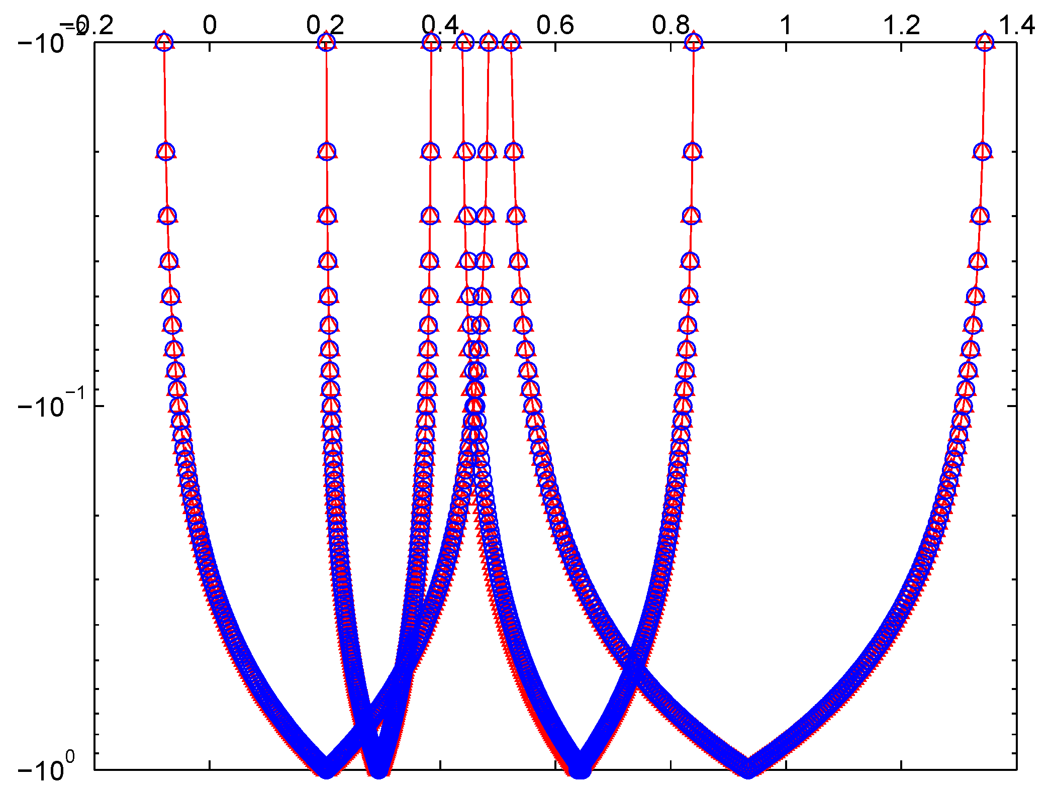
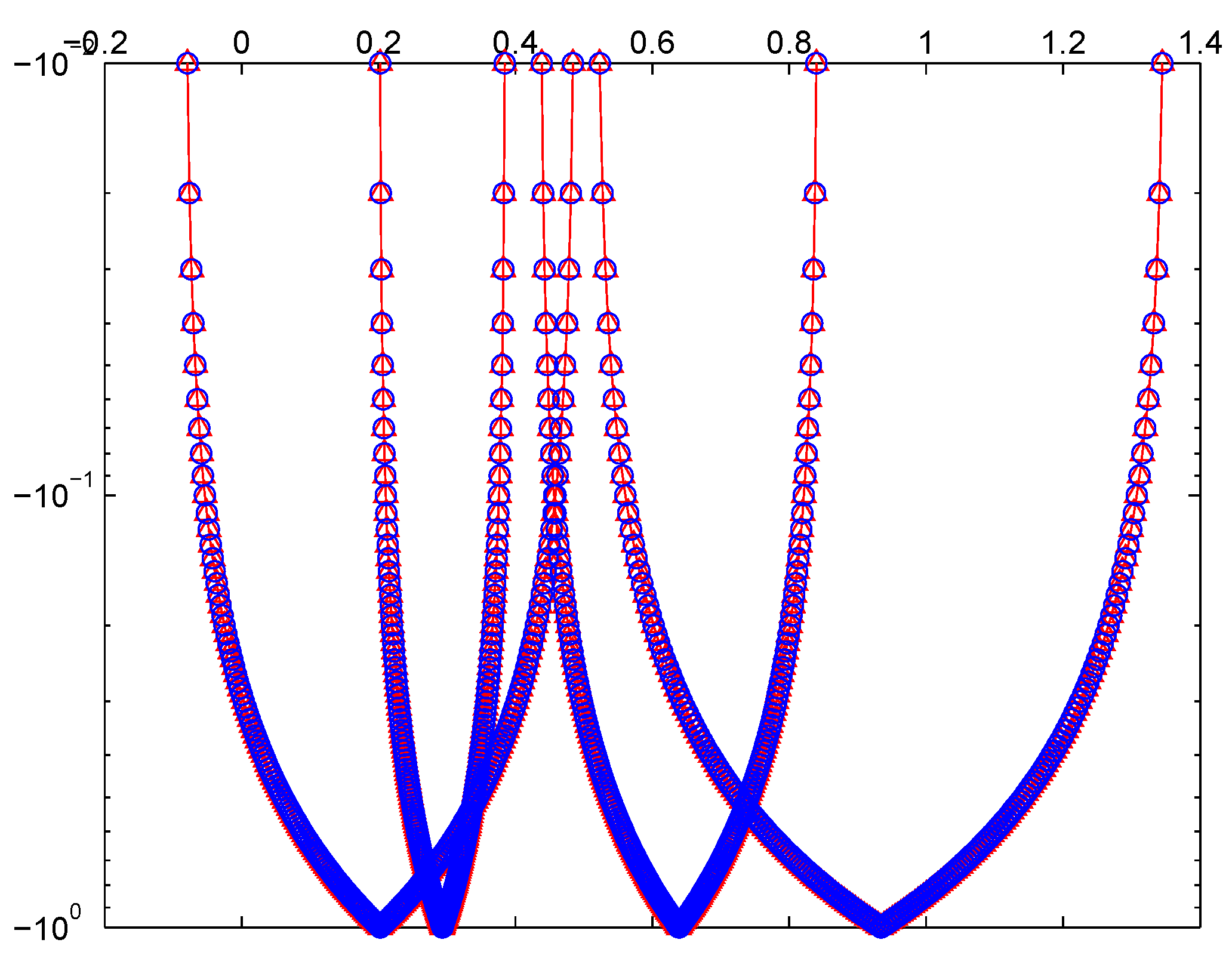
4. Numerical Computations

In Section 4, we discuss the accuracy and efficiency of our considered iterative methods. The following numerical example is considered which has an exact solution.

Example 1.

Consider $4\times 4$ non-symmetric bipolar fuzzy linear system

$$\begin{array}{cc}\hfill 8y_1+y_2-2y_3+y_4& =\langle \left[1+3r,8-4r],[-4s+4,4s+12\right]\rangle ,\hfill \\ \hfill y_1+9y_2+3y_3-y_4& =\langle \left[2+4r,10-4r],[-3s+4,3s+10\right]\rangle ,\hfill \\ \hfill 3y_1+4y_2+11y_3-2y_4& =\langle \left[3+4r,11-4r],[-5s+2,5s+12\right]\rangle ,\hfill \\ \hfill 4y_1-2y_2+3y_3+10y_4& =\langle \left[4+4r,12-4r],[-2s+4,2s+8\right]\rangle .\hfill \end{array}$$

(71)

The extended $16\times 16$ matrix is

$$\begin{array}{c}\hfill Q=\left[\begin{array}{llllllllllllllll}8& 1& 0& 1& 0& 0& 2& 0& 0& 0& 0& 0& 0& 0& 0& 0\\ 1& 9& 3& 0& 0& 0& 0& 1& 0& 0& 0& 0& 0& 0& 0& 0\\ 3& 4& 11& 0& 0& 0& 0& 2& 0& 0& 0& 0& 0& 0& 0& 0\\ 4& 0& 3& 10& 0& 2& 0& 0& 0& 0& 0& 0& 0& 0& 0& 0\\ 0& 0& 0& 0& 0& 0& 0& 0& 8& 1& 0& 1& 0& 0& 2& 0\\ 0& 0& 0& 0& 0& 0& 0& 0& 1& 9& 3& 0& 0& 0& 0& 1\\ 0& 0& 0& 0& 0& 0& 0& 0& 3& 4& 11& 0& 0& 0& 0& 2\\ 0& 0& 0& 0& 0& 0& 0& 0& 4& 0& 3& 10& 0& 2& 0& 0\\ 0& 0& 2& 0& 8& 1& 0& 1& 0& 0& 0& 0& 0& 0& 0& 0\\ 0& 0& 0& 1& 1& 9& 3& 0& 0& 0& 0& 0& 0& 0& 0& 0\\ 0& 0& 0& 2& 3& 4& 11& 0& 0& 0& 0& 0& 0& 0& 0& 0\\ 0& 2& 0& 0& 4& 0& 3& 10& 0& 0& 0& 0& 0& 0& 0& 0\\ 0& 0& 0& 0& 0& 0& 0& 0& 0& 0& 2& 0& 8& 1& 0& 1\\ 0& 0& 0& 0& 0& 0& 0& 0& 0& 0& 0& 1& 1& 9& 3& 0\\ 0& 0& 0& 0& 0& 0& 0& 0& 0& 0& 0& 2& 3& 4& 11& 0\\ 0& 0& 0& 0& 0& 0& 0& 0& 0& 2& 0& 0& 4& 0& 3& 10\end{array}\right],Y=\left[\begin{array}{l}{\underline{y}}_1\\ {\underline{y}}_2\\ {\underline{y}}_3\\ {\underline{y}}_4\\ {\underline{y}}_1^{{}^{\prime }}\\ {\underline{y}}_2^{{}^{\prime }}\\ {\underline{y}}_3^{{}^{\prime }}\\ {\underline{y}}_4^{{}^{\prime }}\\ {\overline{y}}_1\\ {\overline{y}}_2\\ {\overline{y}}_3\\ {\overline{y}}_4\\ {\overline{y}}_1^{{}^{\prime }}\\ {\overline{y}}_2^{{}^{\prime }}\\ {\overline{y}}_3^{{}^{\prime }}\\ {\overline{y}}_4^{{}^{\prime }}\end{array}\right],Z=\left[\begin{array}{l}1+3r\\ 2+4r\\ 3+4r\\ 4+4r\\ -4s+4\\ -3s+4\\ -5s+2\\ -2s+4\\ 8-4r\\ 10-4r\\ 11-4r\\ 12-4r\\ 4s+12\\ 3s+10\\ 5s+12\\ 2s+8\end{array}\right].\end{array}$$

(72)

The exact solution is

$$\begin{array}{cc}\hfill y_1=& ({\underline{y}}_1,{\overline{y}}_1),y_1^{{}^{\prime }}=({\underline{y}}_1^{{}^{\prime }},{\overline{y}}_1^{{}^{\prime }}),y_2=({\underline{y}}_2,{\overline{y}}_2),y_2^{{}^{\prime }}=({\underline{y}}_2^{{}^{\prime }},{\overline{y}}_2^{{}^{\prime }}),\hfill \\ \hfill y_3=& ({\underline{y}}_3,{\overline{y}}_3),y_3^{{}^{\prime }}=({\underline{y}}_3^{{}^{\prime }},{\overline{y}}_3^{{}^{\prime }}),y_4=({\underline{y}}_4,{\overline{y}}_4),y_4^{{}^{\prime }}=({\underline{y}}_4^{{}^{\prime }},{\overline{y}}_4^{{}^{\prime }}),\hfill \end{array}$$

(73)

where

$$\begin{array}{c}\left[\begin{array}{c}{\underline{y}}_1\\ {\underline{y}}_2\\ {\underline{y}}_3\\ {\underline{y}}_4\\ {\underline{y}}_1^{{}^{\prime }}\\ {\underline{y}}_2^{{}^{\prime }}\\ {\underline{y}}_3^{{}^{\prime }}\\ {\underline{y}}_4^{{}^{\prime }}\end{array}\right]=\left[\begin{array}{c}{\displaystyle \frac{205,281,797,262,506,111}{115,292,150,406,846,976}}+{\displaystyle \frac{41,106,967,245,497,243r}{144,115,188,075,855,872}}\\ {\displaystyle \frac{216,257,760,951,346,509}{1,152,921,504,606,846,976}}+{\displaystyle \frac{814,629,203,203,909,695r}{2,305,843,009,213,693,952}}\\ {\displaystyle \frac{333,881,070,289,899,549}{1,152,921,504,606,846,976}}+{\displaystyle \frac{152,372,533,207,200,369r}{1,152,921,504,606,846,976}}\\ {\displaystyle \frac{60,490,739,861,518,559}{144,115,188,075,855,872}}+{\displaystyle \frac{12,724,666,385,266,603r}{72,057,594,037,927,936}}\\ -{\displaystyle \frac{478,534,457,670,319,181s}{1,152,921,504,606,846,976}}+{\displaystyle \frac{299,195,306,676,559,167}{576,460,752,303,423,488}}\\ -{\displaystyle \frac{14,601,336,177,898,265s}{72,057,594,037,927,936}}+{\displaystyle \frac{251,586,656,301,268,601}{576,460,752,303,423,488}}\\ -{\displaystyle \frac{655,697,336,628,817,977s}{2,305,843,009,213,693,952}}-{\displaystyle \frac{94,298,652,911,735,839}{1,152,921,504,606,846,976}}\\ {\displaystyle \frac{52,954,179,205,177,697s}{576,460,752,303,423,488}}+{\displaystyle \frac{111,046,291,608,517,119}{288,230,376,151,711,744}}\end{array}\right],\end{array}$$

(74)

$$\begin{array}{c}\hfill \left[\begin{array}{c}{\overline{y}}_1\\ {\overline{y}}_2\\ {\overline{y}}_3\\ {\overline{y}}_4\\ {\overline{y}}_1^{{}^{\prime }}\\ {\overline{y}}_2^{{}^{\prime }}\\ {\overline{y}}_3^{{}^{\prime }}\\ {\overline{y}}_4^{{}^{\prime }}\end{array}\right]=\left[\begin{array}{c}{\displaystyle \frac{4,009,280,272,373,517,833}{4,611,686,018,427,387,904}}-{\displaystyle \frac{1,872,730,131,467,581,607r}{4,611,686,018,427,387,904}}\\ {\displaystyle \frac{16,402,748,563,310,565,837}{18,446,744,073,709,551,616}}-{\displaystyle \frac{6,425,590,762,457,744,143r}{18,446,744,073,709,551,616}}\\ {\displaystyle \frac{594,758,276,668,348,435}{1,152,921,504,606,846,976}}-{\displaystyle \frac{108,504,673,171,248,555r}{1,152,921,504,606,846,976}}\\ {\displaystyle \frac{105,925,230,935,078,673}{144,115,188,075,855,872}}-{\displaystyle \frac{39,970,316,606,053,779r}{288,230,376,151,711,744}}\\ {\displaystyle \frac{3,828,275,661,362,553,255s}{9,223,372,036,854,775,808}}+{\displaystyle \frac{622,183,811,4775,026,633}{4,611,686,018,427,387,904}}\\ {\displaystyle \frac{7,475,884,123,083,911,711s}{36,893,488,147,419,103,232}}+{\displaystyle \frac{7,763,328,562,362,253,455}{9,223,372,036,854,775,808}}\\ {\displaystyle \frac{655,697,336,628,817,957s}{2,305,843,009,213,693,952}}+{\displaystyle \frac{280,699,341,858,541,055}{576,460,752,303,423,488}}\\ -{\displaystyle \frac{13,238,544,801,294,421s}{144,115,188,075,855,872}}+{\displaystyle \frac{29,046,056,201,669,725}{144,115,188,075,855,872}}\end{array}\right].\end{array}$$

(75)

The graphically representation of exact solution is shown in Figure 1 and Figure 2, respectively.

Using MATLAB software (R2014a, MathWorks, Natick, MA, USA), we obtain the approximate solution by using Jacobi iterative method. After 20 iterations.

$$\begin{array}{c}{\left[\begin{array}{cc}{Y}^{20}& Y^{{}^{\prime }20}\end{array}\right]}^t={\left[\begin{array}{cccccccc}{y}_1& y_2& y_3& y_4& y_1^{{}^{\prime }}& y_2^{{}^{\prime }}& y_3^{{}^{\prime }}& y_4^{{}^{\prime }}\end{array}\right]}^t=\\ \left[\begin{array}{c}{\displaystyle {\displaystyle \frac{12,836,348,501,233,609}{72,057,594,037,927,936}}+{\displaystyle \frac{10,273,623,725,716,725r}{36,028,797,018,963,968}},{\displaystyle \frac{62,638,768,085,732,445}{72,057,594,037,927,936}}-{\displaystyle \frac{117,020,688,532,261,537r}{288,230,376,151,711,744}}}\\ {\displaystyle {\displaystyle \frac{15,213,351,076,053,697}{81,064,793,292,668,928}}+{\displaystyle \frac{114,526,322,656,429,345r}{324,259,173,170,675,712}},{\displaystyle \frac{72,074,663,884,070,117}{81,064,793,292,668,928}}-{\displaystyle \frac{28,229,732,143,909,081r}{81,064,793,292,668,928}}}\\ {\displaystyle {\displaystyle \frac{5,219,075,782,822,605}{18,014,398,509,481,984}}+{\displaystyle \frac{26,165,004,492,231,101r}{198,158,383,604,301,824}}{\displaystyle \frac{12,775,006,769,174,063}{24,769,797,950,537,728}}-{\displaystyle \frac{1,693,201,459,101,159r}{18,014,398,509,481,984}}}\\ {\displaystyle {\displaystyle \frac{75,637,304,041,309,041}{180,143,985,094,819,840}}+{\displaystyle \frac{31,787,786,747,500,183r}{180,143,985,094,819,840}},{\displaystyle \frac{16,547,832,431,431,383}{22,517,998,136,852,480}}-{\displaystyle \frac{12,478,784,331,320,917r}{90,071,992,547,409,920}}}\\ {\displaystyle {\displaystyle \frac{74,810,708,464,573,255}{144,115,188,075,855,872}}-{\displaystyle \frac{239,219,701,678,619,317s}{576,460,752,303,423,488}},{\displaystyle \frac{97,210,279,651,941,455}{72,057,594,037,927,936}}+{\displaystyle \frac{239,219,701,678,619,317s}{576,460,752,303,423,488}}}\\ {\displaystyle {\displaystyle \frac{283,093,879,214,121,889}{648,518,346,341,351,424}}-{\displaystyle \frac{131,353,134,683,459,941s}{648,518,346,341,351,424}},{\displaystyle \frac{682,250,185,726,302,190}{810,647,932,926,689,280}}+{\displaystyle \frac{131,353,134,683,459,941s}{648,518,346,341,351,424}}}\\ {\displaystyle {\displaystyle \frac{16,184,693,616,721,323}{198,158,383,604,301,824}}-{\displaystyle \frac{112,652,205,044,970,927s}{396,316,767,208,603,648}},{\displaystyle \frac{482,337,557,141,248,010}{990,791,918,021,509,120}}+{\displaystyle \frac{112,652,205,044,970,927s}{396,316,767,208,603,648}}}\\ {\displaystyle {\displaystyle \frac{277,706,723,605,062,227}{720,575,940,379,279,360}}+{\displaystyle \frac{16,570,929,654,614,219s}{180,143,985,094,819,840}},{\displaystyle \frac{7,256,964,318,407,423}{360,287,970,189,639,681}}-{\displaystyle \frac{16,570,929,654,614,219s}{180,143,985,094,819,840}}}\end{array}\right],\end{array}$$

(76)

where the bipolar fuzzy variables satisfied the Equation (73). The exact and approximate solutions (EASs) by using the Jacobi iterative scheme are shown in Figure 3 and Figure 4, respectively.

Using MATLAB software, we obtained the approximate solution by using JOR iterative scheme. After 10 iterations with $\alpha =0.80$, we get

$$\begin{array}{c}{\left[\begin{array}{cc}{Y}^{10}& Y^{{}^{\prime }10}\end{array}\right]}^t={\left[\begin{array}{cccccccc}{y}_1& y_2& y_3& y_4& y_1^{{}^{\prime }}& y_2^{{}^{\prime }}& y_3^{{}^{\prime }}& y_4^{{}^{\prime }}\end{array}\right]}^t=\\ \left[\begin{array}{c}{\displaystyle {\displaystyle \frac{64,183,538,040,639,217}{360,287,970,189,639,680}}+{\displaystyle \frac{205,470,694,833,247,005r}{72,057,594,037,927,936}},{\displaystyle \frac{782,986,996,752,688,007}{90,071,992,547,409,920}}-{\displaystyle \frac{73,137,956,621,906,247r}{180,143,985,094,819,840}}}\\ {\displaystyle {\displaystyle \frac{304,377,676,954,972,063}{162,129,586,585,337,856}}+{\displaystyle \frac{71,567,293,554,241,673r}{202,661,983,231,672,320}},{\displaystyle \frac{360,355,368,548,603,279}{405,323,966,463,344,640}}-{\displaystyle \frac{282,252,724,402,753,831r}{810,647,932,926,689,280}}}\\ {\displaystyle {\displaystyle \frac{143,345,510,986,740,351}{495,395,959,010,754,560}}+{\displaystyle \frac{4,768,569,534,855,033r}{36,028,797,018,963,968}},{\displaystyle \frac{116,191,998,055,430,670}{225,179,981,368,524,800}}-{\displaystyle \frac{373,672,429,047,603,413r}{396,316,767,208,603,648}}}\\ {\displaystyle {\displaystyle \frac{11,813,590,477,185,047}{281,474,976,710,656}}+{\displaystyle \frac{7,953,6798,356,010,267r}{450,359,962,737,049,600}},{\displaystyle \frac{165,505,486,411,360,901}{225,179,981,368,524,800}}-{\displaystyle \frac{124,913,453,663,501,531r}{900,719,925,474,099,200}}}\\ {\displaystyle -{\displaystyle \frac{299,074,581,675,723,373s}{720,575,940,379,279,360}}+{\displaystyle \frac{934,998,169,741,259,007}{1,801,439,850,948,198,400}},{\displaystyle \frac{60,759,276,952,996,901}{45,035,996,273,704,960}}+{\displaystyle \frac{299,074,581,675,723,373s}{720,575,940,379,279,360}}}\\ {\displaystyle -{\displaystyle \frac{657,032,887,796,021,003s}{324,259,173,170,675,712}}+{\displaystyle \frac{353,838,414,776,193,103}{810,647,932,926,689,280}},{\displaystyle \frac{341,177,429,337,101,801}{405,323,966,463,344,640}}+{\displaystyle \frac{657,032,887,796,021,003s}{324,259,173,170,675,712}}}\\ {\displaystyle -{\displaystyle \frac{140,868,228,790,242,821s}{495,395,959,010,754,560}}-{\displaystyle \frac{324,694,771,895,893,627}{396,316,767,208,603,648}},{\displaystyle \frac{482,299,222,186,997,837}{990,791,918,021,509,120}}+{\displaystyle \frac{140,868,228,790,242,821s}{495,395,959,010,754,560}}}\\ {\displaystyle {\displaystyle \frac{165,451,141,212,943,659s}{1,801,439,850,948,198,400}}+{\displaystyle \frac{346,972,928,656,974,293}{900,719,925,474,099,200}},{\displaystyle \frac{181,521,787,444,030,587}{900,719,925,474,099,200}}-{\displaystyle \frac{165,451,141,212,943,659s}{1,801,439,850,948,198,400}}}\end{array}\right],\end{array}$$

(77)

where the bipolar fuzzy variables satisfied the Equation (73). The EASs by using the JOR iterative scheme are shown in Figure 5 and Figure 6, respectively.

Using MATLAB software, we obtain the approximate solution by using GS iterative scheme. After 20 iterations.

$$\begin{array}{c}{\left[\begin{array}{cc}{Y}^{20}& Y^{{}^{\prime }20}\end{array}\right]}^t={\left[\begin{array}{cccccccc}{y}_1& y_2& y_3& y_4& y_1^{{}^{\prime }}& y_2^{{}^{\prime }}& y_3^{{}^{\prime }}& y_4^{{}^{\prime }}\end{array}\right]}^t=\\ \left[\begin{array}{c}{\displaystyle {\displaystyle \frac{51,320,449,316,232,361}{288,230,376,151,711,744}}+{\displaystyle \frac{41,106,967,245,505,807r}{144,115,188,075,855,872}},{\displaystyle \frac{31,322,502,127,996,295}{36,028,797,018,963,968}}-{\displaystyle \frac{29,261,408,304,181,595r}{72,057,594,037,927,936}}}\\ {\displaystyle {\displaystyle \frac{486,579,962,138,207,351}{259,407,338,536,540,569}}+{\displaystyle \frac{458,228,926,802,296,721r}{129,703,669,268,270,284}},{\displaystyle \frac{288,329,564,589,184,129}{324,259,173,170,675,712}}-{\displaystyle \frac{125,499,819,579,260,003r}{360,287,970,189,639,680}}}\\ {\displaystyle {\displaystyle \frac{8,263,556,489,616,166,609}{28,534,807,239,019,462,656}}+{\displaystyle \frac{1,885,610,098,436,760,775r}{142,674,036,195,097,313,280}},{\displaystyle \frac{167,275,765,312,253,605}{324,259,173,170,675,712}}-{\displaystyle \frac{745,969,628,052,397,007r}{792,633,534,417,207,296}}}\\ {\displaystyle {\displaystyle \frac{7,984,777,661,677,934,671}{19,023,204,826,012,975,104}}+{\displaystyle \frac{839,827,981,427,528,153r}{475,580,120,650,324,377}},{\displaystyle \frac{794,439,232,010,721,113}{108,086,391,056,891,904}}-{\displaystyle \frac{1,099,183,706,666,935,019r}{792,633,534,417,207,296}}}\\ {\displaystyle {\displaystyle \frac{584,365,833,354,731}{1,125,899,906,842,624}}-{\displaystyle \frac{239,267,228,835,244,237s}{576,460,752,303,423,488}},{\displaystyle \frac{388,864,882,174,055,383}{288,230,376,151,711,744}}+{\displaystyle \frac{239,267,228,835,244,237s}{576,460,752,303,423,488}}}\\ {\displaystyle {\displaystyle \frac{572,414,568,074,145,737}{1,297,036,692,682,702,848}}-{\displaystyle \frac{66,514,702,189,282,229s}{324,259,173,170,675,712}},{\displaystyle \frac{2,183,436,158,161,561,321}{259,407,338,536,540,569}}+{\displaystyle \frac{350,432,068,270,000,121s}{172,938,225,691,027,046}}}\\ {\displaystyle -{\displaystyle \frac{145,868,228,724,373,097}{1783,425,452,438,716,416}}-{\displaystyle \frac{491,773,002,471,150,725s}{172,938,225,691,027,046}},{\displaystyle \frac{13,894,617,421,958,003,759}{28,534,807,239,019,462,656}}+{\displaystyle \frac{491,773,002,471,150,725s}{172,938,225,691,027,046}}}\\ {\displaystyle {\displaystyle \frac{458,065,952,882,892,877}{1,188,950,301,625,810,944}}+{\displaystyle \frac{105,908,358,410,378,693s}{1,152,921,504,606,846,976}},{\displaystyle \frac{3,834,079,418,583,789,233}{190,232,048,260,129,751}}-{\displaystyle \frac{105,908,358,410,378,693s}{115,292,150,460,684,697}}}\end{array}\right],\end{array}$$

(78)

where the bipolar fuzzy variables satisfied the Equation (73). The EASs by using the GS iterative scheme are shown in Figure 7 and Figure 8, respectively.

Using MATLAB software, we obtain the approximate solution by using EGS iterative scheme. After 10 iterations with $\alpha =0.90$ gives

$$\begin{array}{c}{\left[\begin{array}{cc}{Y}^{10}& Y^{{}^{\prime }10}\end{array}\right]}^t={\left[\begin{array}{cccccccc}{y}_1& y_2& y_3& y_4& y_1^{{}^{\prime }}& y_2^{{}^{\prime }}& y_3^{{}^{\prime }}& y_4^{{}^{\prime }}\end{array}\right]}^t=\\ \left[\begin{array}{c}{\displaystyle {\displaystyle \frac{513,214,280,517,023,290}{288,230,376,151,711,744}}+{\displaystyle \frac{102,767,283,537,499,967r}{360,287,970,189,639,680}},{\displaystyle \frac{156,612,990,212,095,999}{180,143,985,094,819,840}}-{\displaystyle \frac{234,091,058,915,302,597r}{576,460,752,303,423,488}}}\\ {\displaystyle {\displaystyle \frac{270,322,998,174,536,579}{144,115,188,075,855,872}}+{\displaystyle \frac{63,642,787,775,584,381r}{180,143,985,094,819,840}},{\displaystyle \frac{800,914,578,339,196,93}{900,719,925,474,099,200}}-{\displaystyle \frac{1,003,996,049,927,006,947r}{288,230,376,151,711,744}}}\\ {\displaystyle {\displaystyle \frac{827,002,061,040,401,072,744,797,145,506,906,470}{285,576,327,219,415,519,569,177,298,107,105,280}}+{\displaystyle \frac{754,849,284,553,644,456,757,715,327,792,466r}{571,152,654,438,831,039,138,354,596,214,210,560}}},\\ {\displaystyle {\displaystyle \frac{736,596,232,171,698,680,055,576,906,871,720,099}{142,788,163,609,707,759,784,588,649,053,552,640}}-{\displaystyle \frac{335,957,201,282,717,580,827,543,168,533,989r}{356,970,409,024,269,399,461,471,622,633,881,060}}}\\ {\displaystyle {\displaystyle \frac{66,539,221,211,736,877,141}{158,526,706,883,441,459,200}}+{\displaystyle \frac{699,857,903,859,994,436r}{39,631,676,720,860,364,800}},{\displaystyle \frac{14,564,658,402,701,290,359}{19,815,838,360,430,182,400}}-{\displaystyle \frac{87,934,919,421,894,666,610r}{634,106,827,533,765,836,800}}}\\ {\displaystyle -{\displaystyle \frac{598,166,266,984,383,857s}{144,115,188,075,855,872}}+{\displaystyle \frac{116,874,220,233,318,017}{225,179,981,368,524,800}},{\displaystyle \frac{972,163,771,731,002,001}{720,575,940,379,279,360}}+{\displaystyle \frac{598,166,266,984,383,857s}{144,115,188,075,855,872}}}\\ {\displaystyle {\displaystyle \frac{157,242,095,178,192,669}{360,287,970,189,639,680}}-{\displaystyle \frac{58,404,495,278,051,387s}{2,882,303,761,517,117,404}}{\displaystyle \frac{606,506,666,7466,422,183}{720,575,940,379,279,360}}+{\displaystyle \frac{584,044,952,780,513,087s}{288,230,376,151,711,744}}}\\ {\displaystyle -{\displaystyle \frac{406,039,028,833,267,449,730,391,838,693,565,207s}{142,788,163,609,707,759,784,588,649,053,552,640}}-{\displaystyle \frac{583,968,217,167,055,772,899,295,380,199,581}{713,940,818,0485,387,989,229,432,452,677,632}}},\\ {\displaystyle {\displaystyle \frac{869,105,517,791,404,670,742,876,608,731,877}{178,485,204,512,134,699,730,735,811,316,940,800}}+{\displaystyle \frac{406,039,028,833,267,449,730,391,838,693,565,207s}{142,788,163,609,707,759,784,588,649,053,552,640}}}\\ {\displaystyle {\displaystyle \frac{763,432,587,573,703,351}{198,158,383,604,301,824}}+{\displaystyle \frac{145,620,989,572,932,492,407s}{158,526,706,883,441,459,200}},{\displaystyle \frac{15,975,204,545,654,884,073}{792,633,534,417,207,296}}-{\displaystyle \frac{145,620,989,572,932,492,407s}{158,526,706,883,441,459,200}}}\end{array}\right],\end{array}$$

(79)

where the bipolar fuzzy variables satisfied the Equation (73). The EASs by using the EGS iterative scheme are shown in Figure 9 and Figure 10, respectively.

Using MATLAB software, we obtain the approximate solution by using SOR iterative scheme. After 10 iterations with $\omega =1.25$ gives

$$\begin{array}{c}{\left[\begin{array}{cc}{Y}^{10}& Y^{{}^{\prime }10}\end{array}\right]}^t={\left[\begin{array}{cccccccc}{y}_1& y_2& y_3& y_4& y_1^{{}^{\prime }}& y_2^{{}^{\prime }}& y_3^{{}^{\prime }}& y_4^{{}^{\prime }}\end{array}\right]}^t=\\ \left[\begin{array}{c}{\displaystyle {\displaystyle \frac{256,587,866,905,801,003}{144,115,188,075,855,872}}+{\displaystyle \frac{164,428,183,756,680,425r}{576,460,752,303,423,488}},{\displaystyle \frac{626,443,024,737,125,507}{72,057,594,037,927,936}}-{\displaystyle \frac{468,182,178,541,392,089r}{1,115,292,150,460,684,697}}}\\ {\displaystyle {\displaystyle \frac{973,314,999,560,092,481}{5,188,146,770,730,811,392}}+{\displaystyle \frac{7,331,632,359,384,465,395r}{20,752,587,082,923,245,568}},{\displaystyle \frac{230,671,790,274,240,135}{2,594,073,385,365,405,696}}-{\displaystyle \frac{481,923,390,954,291,749r}{13,835,058,055,282,163,712}}}\\ {\displaystyle {\displaystyle \frac{8,026,367,316,189,065,662}{28,534,807,239,019,462,656}}+{\displaystyle \frac{15,084,841,908,753,476,377r}{114,139,228,956,077,850,624}},{\displaystyle \frac{7,360,191,262,212,243,823}{142,674,036,195,097,313,280}}-{\displaystyle \frac{716,133,036,092,123,217r}{76,092,819,304,051,900,416}}}\\ {\displaystyle {\displaystyle \frac{31,937,325,129,223,539,737}{76,092,819,304,051,900,416}}+{\displaystyle \frac{53,749,973,947,897,126,943r}{304,371,277,216,207,601,664}},{\displaystyle \frac{79,634,402,288,248,334,997}{38,464,096,520,259,502,008}}-{\displaystyle \frac{28,138,831,577,204,920,765r}{202,914,184,810,805,067,776}}}\\ {\displaystyle -{\displaystyle \frac{239,267,784,010,105,947s}{576,460,752,303,423,488}}+{\displaystyle \frac{149,591,412,441,401,513}{288,230,376,151,711,744}},{\displaystyle \frac{155,543,678,580,602,985}{1,152,921,504,606,846,976}}+{\displaystyle \frac{239,267,784,010,105,947s}{576,460,752,303,423,488}}}\\ {\displaystyle -{\displaystyle \frac{420,519,441,769,687,720s}{20,752,587,082,923,245,568}}+{\displaystyle \frac{4,529,386,962,991,141,867}{103,762,935,414,616,227,804}},{\displaystyle \frac{388,203,616,919,467,516,7}{4,461,168,601,842,738,794}}+{\displaystyle \frac{420,519,441,769,687,720s}{20,752,587,082,923,245,568}}}\\ {\displaystyle -{\displaystyle \frac{324,569,890,425,472,481,603s}{114,139,228,956,077,850,624}}-{\displaystyle \frac{4,466,705,784,611,433,495}{570,696,144,780,389,253,102}},{\displaystyle \frac{13,510,805,317,479,615,225}{25,642,731,013,506,334,472}}+{\displaystyle \frac{3,245,698,9042,547,248,163s}{114,139,228,956,077,850,624}}}\\ {\displaystyle {\displaystyle \frac{27,959,467,995,013,168,763s}{304,371,277,216,207,601,664}}+{\displaystyle \frac{58,621,246,560,010,170,595}{152,185,638,608,103,800,832}},{\displaystyle \frac{40,882,371,419,995,997,481}{202,914,184,810,805,067,776}}-{\displaystyle \frac{27,959,467,995,013,168,763s}{304,371,277,216,207,601,664}}}\end{array}\right],\end{array}$$

(80)

where the bipolar fuzzy variables satisfied the Equation (73). The EASs by using the forward SOR iterative scheme are shown in Figure 11 and Figure 12, respectively.

Comparison Analysis of Proposed Methods

Comparison results for Example 1 are shown in

Table 1. Comparison analysis.

Comparison Results for Example 1
Method	Parameter	Number of Iterations	Distance Based on Housdorff Metric
Jacobi		20	$1.3256\times {10}^{-4}$
JOR	$\alpha =0.80$	10	$2.4023\times {10}^{-4}$
GS		20	$2.2492\times {10}^{-6}$
EGS	$\alpha =0.90$	10	$5.1139\times {10}^{-6}$
SOR	$\omega =1.25$	10	$3.1374\times {10}^{-5}$

. It is easy to see that Jacobi method and GS method converge after 20 iterations, while the JOR method and EGS method converge after 10 iterations for $\alpha =0.8$ and $\alpha =0.9$, respectively. Also, the SOR method converges after 10 iterations for $\alpha$ = 1.25. Consequently, the SOR method is more accurate as compared to the other iterative methods.

5. Conclusions

Iterative methods such as Richardson, ER, Jacobi, JOR, GS, EGS and SOR have attracted our attention to those problems which have no analytical solution in the bipolar fuzzy environment. These iterative methods are used to find the approximate solution of bipolar fuzzy linear system of equations. Since it is more difficult to solve the BFLSEs analytically. To show the validity and accuracy of these iterative methods, an example of having an exact solution is illustrated. In the SOR scheme, for $\omega \in (0,1)$, the method can be used to find the convergence of the system that is not convergent by GS scheme. For $\omega >1$, this choice is used to accelerate the convergence of the system that is already convergent by GS scheme. The numerical example shows that by selecting a good SOR parameter, we can overcome GS method difficulty. We have already found in Table 1 that SOR method is useful for solving the system than the other ones. In the future, we plan to extend our research work to (i) bipolar fuzzy systems of linear equations with polynomial parametric form, and (ii) bipolar fuzzy differential equations.

References

1. Zadeh, L.A. Fuzzy sets. Inf. Control 1965, 8, 338–353. [Google Scholar] [CrossRef] [Green Version]
2. Dubois, D.; Prade, H. Operations on fuzzy numbers. Int. J. Syst. Sci. 1978, 9, 613–626. [Google Scholar] [CrossRef]
3. Dubois, D.; Prade, H. Fuzzy number: An overview. In The Analysis of fuzzy Information, 1: Mathematics; Bezdek, J.C., Ed.; CRC Press: Boca Raton, FL, USA, 1987; pp. 3–39. [Google Scholar]
4. Mizumoto, M.; Tanaka, K. The four operations of arithmetic on fuzzy numbers. Syst. Comput. Controls 1976, 7, 73–81. [Google Scholar]
5. Mizumoto, M.; Tanaka, K. Some properties of fuzzy numbers. In Advances in Fuzzy Set Theory and Applications; Gupta, M.M., Ragade, R.K., Yager, R.R., Eds.; North-Holland: Amsterdam, The Netherlands, 1979; pp. 156–164. [Google Scholar]
6. Nahmias, S. Fuzzy variables. Fuzzy Sets Syst. 1978, 1, 97–111. [Google Scholar] [CrossRef]
7. Goetschel, R.; Voxman, W. Elementary calculus. Fuzzy Sets Syst. 1986, 18, 31–43. [Google Scholar] [CrossRef]
8. Moghadam, K.G.; Ghanbari, R.; Amiri, N.M. Duality in bipolar triangular fuzzy number quadratic programming problems. In Proceedings of the International Conference on Intelligent Sustainable Systems, Palladam, Tirupur, India, 7–8 December 2017; pp. 1236–1238. [Google Scholar]
9. Congxin, W.; Ming, M. On embedding problem of fuzzy number spaces. Fuzzy Sets Syst. 1991, 44, 33–38. [Google Scholar] [CrossRef]
10. Puri, M.L.; Ralescu, D. Differential for fuzzy function. J. Math. Anal. Appl. 1983, 91, 552–558. [Google Scholar] [CrossRef]
11. Buckley, J.J. Fuzzy eigenvalues and input–output analysis. Fuzzy Sets Syst. 1990, 34, 187–195. [Google Scholar] [CrossRef]
12. Diamond, P. Fuzzy least squares. Inf. Sci. 1988, 46, 144–157. [Google Scholar] [CrossRef]
13. Friedman, M.; Ming, M.; Kandel, A. Fuzzy linear systems. Fuzzy Sets Syst. 1998, 96, 201–209. [Google Scholar] [CrossRef]
14. Allahviraloo, T. Numerical methods for fuzzy system of linear equations. Appl. Math. Comput. 2004, 155, 493–502. [Google Scholar]
15. Allahviranloo, T. Successive over relaxation iterative method for fuzzy system of linear equations. Appl. Math. Comput. 2005, 162, 189–196. [Google Scholar]
16. Dehghan, M.; Hashemi, B. Iterative solution of fuzzy linear systems. Appl. Math. Comput. 2006, 175, 645–674. [Google Scholar] [CrossRef]
17. Ezzati, R. Solving fuzzy linear systems. Soft Comput. 2011, 15, 193–197. [Google Scholar] [CrossRef]
18. Muzzioli, S.; Reynaerts, H. Fuzzy linear systems of the form A1x + b1 = A2x + b2. Fuzzy Sets Syst. 2006, 157, 939–951. [Google Scholar] [CrossRef]
19. Allahviranloo, T. A comment on fuzzy linear systems. Fuzzy Sets Syst. 2003, 140, 559. [Google Scholar] [CrossRef]
20. Allahviranloo, T.; Kermani, M.A. Solution of a fuzzy system of linear equation. Appl. Math. Comput. 2006, 175, 519–531. [Google Scholar] [CrossRef]
21. Allahviranloo, T.; Ahmady, E.; Ahmady, N.; Alketaby, K.S. Block Jacobi two-stage method with Gauss-Sidel inner iterations for fuzzy system of linear equations. Appl. Math. Comput. 2006, 175, 1217–1228. [Google Scholar] [CrossRef]
22. Abbasbandy, S.; Jafarian, A. Steepest descent method for system of fuzzy linear equations. Appl. Math. Comput. 2006, 175, 823–833. [Google Scholar] [CrossRef]
23. Ineirat, L. Numerical Methods for Solving Fuzzy System of Linear Equations. Master’s Thesis, An-Najah National University, Nablus, Palestine, 2017. [Google Scholar]
24. Asady, B.; Abbasbandy, S.; Alavi, M. Fuzzy general linear systems. Appl. Math. Comput. 2005, 169, 34–40. [Google Scholar] [CrossRef]
25. Dubois, D.; Prade, H. An introduction to bipolar representations of information and preference. Int. J. Intell. Syst. 2008, 23, 866–877. [Google Scholar] [CrossRef]
26. Zhang, W.R. Bipolar fuzzy sets. In Proceedings of the IEEE International Conference on Fuzzy Systems Proceedings, Anchorage, AK, USA, 4–9 May 1998; pp. 835–840. [Google Scholar]
27. Zhang, W.R. Bipolar fuzzy sets and relations: A computational framework forcognitive modeling and multiagent decision analysis. In Proceedings of the First International Joint Conference of The North American Fuzzy Information Processing Society Biannual Conference, San Antonio, TX, USA, 18–21 December 1994; pp. 305–309. [Google Scholar]
28. Akram, M. Bipolar fuzzy graphs. Inf. Sci. 2011, 181, 5548–5564. [Google Scholar] [CrossRef]
29. Ali, G.; Akram, M.; Koam, A.N.A.; Alcantud, J.C.R. Parameter reductions of bipolar fuzzy soft sets with their decision-making algorithms. Symmetry 2019, 11, 949. [Google Scholar] [CrossRef]
30. Akram, M.; Luqman, A. Certain concepts of bipolar fuzzy directed hypergraphs. Mathematics 2017, 5, 17. [Google Scholar] [CrossRef]
31. Akram, M.; Arshad, M. A novel trapezoidal bipolar fuzzy topsis method for group decision-making. Group Decis. Negot. 2019, 28, 565–584. [Google Scholar] [CrossRef]
32. Akram, M.; Muhammad, G.; Allahviranloo, T. Bipolar fuzzy linear system of equations. Appl. Math. Comput. 2019, 38, 69. [Google Scholar] [CrossRef]
33. Muhammad, G. Bipolar Fuzzy Linear Systems. M.Phil’s Thesis, Higher Education Commission, Islamabad, Pakistan, 2019. [Google Scholar]
34. Grzegorzewski, P. Distances between intuitionistic fuzzy sets and/or interval-valued fuzzy sets based on the Hausdorff metric. Fuzzy Sets Syst. 2004, 148, 319–328. [Google Scholar] [CrossRef]
35. Hageman, L.A.; Young, D.M. Applied Iterative Methods; Courier Corporation: North Chelmsford, MA, USA, 2012. [Google Scholar]
Figure 1. The exact solution of positive membership of the 4 × 4 bipolar fuzzy linear system of equations.
Mathematics 07 00728 g001
Figure 2. Exact solution of negative membership of 4 × 4 bipolar fuzzy linear system of equations.
Mathematics 07 00728 g002
Figure 3. Compare the exact and approximate solutions (EASs) of positive membership by using the Jacobi iterative technique after 20 iteration of 4 × 4 bipolar fuzzy linear system of equations.
Mathematics 07 00728 g003
Figure 4. Compare the EASs of negative membership by using the Jacobi iterative technique after 20 iteration of 4 × 4 bipolar fuzzy linear system of equations.
Mathematics 07 00728 g004
Figure 5. Compare the EASs of positive membership by using the JOR iterative technique after 10 iteration of 4 × 4 bipolar fuzzy linear system of equations.
Mathematics 07 00728 g005
Figure 6. Compare the EASs of negative membership by using the JOR iterative technique after 10 iteration of 4 × 4 bipolar fuzzy linear system of equations.
Mathematics 07 00728 g006
Figure 7. Compare the EASs of positive membership by using the GS iterative technique after 20 iteration of 4 × 4 bipolar fuzzy linear system of equations.
Mathematics 07 00728 g007
Figure 8. Compare the EASs of negative membership by using the GS iterative technique after 20 iteration of 4 × 4 bipolar fuzzy linear system of equations.
Mathematics 07 00728 g008
Figure 9. Compare the EASs of positive membership by using the EGS iterative technique after 10 iteration of 4 × 4 bipolar fuzzy linear system of equations.
Mathematics 07 00728 g009
Figure 10. Compare the EASs of negative membership by using the EGS iterative technique after 10 iteration of 4 × 4 bipolar fuzzy linear system of equations.
Mathematics 07 00728 g010
Figure 11. Compare the EASs of positive membership by using the SOR forward iterative technique after 10 iteration of 4 × 4 bipolar fuzzy linear system of equations.
Mathematics 07 00728 g011
Figure 12. Compare the EASs of negative membership by using the SOR forward iterative technique after 10 iteration of 4 × 4 bipolar fuzzy linear system of equations.
Mathematics 07 00728 g012