On New Solutions of Time-Fractional Wave Equations Arising in Shallow Water Wave Propagation

Abstract

The primary objective of this manuscript is to obtain the approximate analytical solution of Camassa–Holm (CH), modified Camassa–Holm (mCH), and Degasperis–Procesi (DP) equations with time-fractional derivatives labeled in the Caputo sense with the help of an iterative approach called fractional reduced differential transform method (FRDTM). The main benefits of using this technique are that linearization is not required for this method and therefore it reduces complex numerical computations significantly compared to the other existing methods such as the perturbation technique, differential transform method (DTM), and Adomian decomposition method (ADM). Small size computations over other techniques are the main advantages of the proposed method. Obtained results are compared with the solutions carried out by other technique which demonstrates that the proposed method is easy to implement and takes small size computation compared to other numerical techniques while dealing with complex physical problems of fractional order arising in science and engineering.

1. Introduction

Nonlinear phenomena are of significant importance in natural sciences and engineering. Most of our real-life problems are modeled through the use of nonlinear phenomena. In the present years, fractional calculus has become widespread because of its applications in mathematical biology, electrochemistry, and physics [1,2,3,4,5,6,7,8]. For example, the earthquake model [9] and traffic model [10] with fractional derivatives have been demonstrated. However, sometimes, it is challenging to find the exact and numerical solutions of these models. During the last few decades, several analytical and numerical approaches have been established for the solution of such types of models such as homotopy perturbation method (HPM) [10,11], homotopy perturbation transform method [12,13], homotopy analysis method (HAM) [14,15], Adomian decomposition method (ADM) [16,17], sine-cosine method [18] and transform method [19]. Recently, multi-dimensional diffusion equation of fractional order has been solved by Kumar et al. [20] by modified HPM (m-HPM). In this approach, parameter p has been presented to extend the solution in series form, whereas the nonlinear terms can be extended by using He’s polynomial [21]. It has been observed that the computation of He’s polynomial is complicated, and the main disadvantage of this approach is its complexity in that regard and enormous calculations.

Among all the listed method, FRDTM plays a vital role because it takes small size computation, easy to implement as compared to other techniques. It was first introduced and developed by Keskin and Oturanc [22]. It is a beneficial and powerful semi-analytical approach. By implementation of the FRDTM, many physical nonlinear problems can be solved easily. In this article, the nonlinear time-fractional Camassa–Holm (CH) equation is taken as [23,24]

$$\begin{array}{c}\frac{{\partial }^{\alpha }\psi }{\partial t^{\alpha }}+2c\frac{\partial \psi }{\partial x}-\frac{{\partial }^3\psi }{\partial x^2\partial t}+3\psi \frac{\partial \psi }{\partial x}=2\frac{\partial \psi }{\partial x}\frac{{\partial }^2\psi }{\partial x^2}+\psi \frac{{\partial }^3\psi }{\partial x^3},\\ \mathrm{for}t>0,\hspace{0.17em}x\in \Re ,\hspace{0.17em}0<\alpha \le 1,\end{array}$$

(1)

with initial condition (IC)

$$\psi \left(x,0\right)=g\left(x\right),$$

(1a)

The modified Camassa–Holm (mCH) and Degasperis–Procesi (DP) equations are derived from modified b-equation [25] which is

$$\frac{\partial \psi }{\partial t}-\frac{{\partial }^3\psi }{\partial x^2\partial t}+\left(b+1\right){\psi }^2\frac{\partial \psi }{\partial x}=b\frac{\partial \psi }{\partial x}\frac{{\partial }^2\psi }{\partial x^2}+\psi \frac{{\partial }^3\psi }{\partial x^3}$$

(1b)

where b is a positive integer.

The time-fractional mCH and time-fractional DP are derived from fractional modified b-equation which may be written as

$$\frac{{\partial }^{\alpha }\psi }{\partial t^{\alpha }}-\frac{{\partial }^3\psi }{\partial x^2\partial t}+\left(b+1\right){\psi }^2\frac{\partial \psi }{\partial x}=b\frac{\partial \psi }{\partial x}\frac{{\partial }^2\psi }{\partial x^2}+\psi \frac{{\partial }^3\psi }{\partial x^3}$$

(1c)

By substituting b = 2, b = 3 into Equation (1c), we obtain the time-fractional mCH equation and time-fractional DP equation, respectively. So, the nonlinear time-fractional mCH equation is written as [11,24,25]

$$\frac{{\partial }^{\alpha }\psi }{\partial t^{\alpha }}-\frac{{\partial }^3\psi }{\partial x^2\partial t}+3{\psi }^2\frac{\partial \psi }{\partial x}=2\frac{\partial \psi }{\partial x}\frac{{\partial }^2\psi }{\partial x^2}+\psi \frac{{\partial }^3\psi }{\partial x^3},\mathrm{for}t>0,\hspace{0.17em}x\in \Re ,\hspace{0.17em}0<\alpha \le 1$$

(2)

with IC

$$\psi \left(x,0\right)=p\left(x\right),$$

(2a)

and the nonlinear time-fractional DP equation is given as [11,24,25]

$$\frac{{\partial }^{\alpha }\psi }{\partial t^{\alpha }}-\frac{{\partial }^3\psi }{\partial x^2\partial t}+4{\psi }^2\frac{\partial \psi }{\partial x}=3\frac{\partial \psi }{\partial x}\frac{{\partial }^2\psi }{\partial x^2}+\psi \frac{{\partial }^3\psi }{\partial x^3},\mathrm{for}t>0,\hspace{0.17em}x\in \Re ,\hspace{0.17em}0<\alpha \le 1$$

(3)

with IC

$$\psi \left(x,0\right)=f\left(x\right),$$

(3a)

These three models are the unidirectional shallow water waves propagation over a flat bottom. Equation (1) is a shallow water wave equation and was initially determined as an estimation to the incompressible Euler equation and observed to be integrable with a Lax pair [26]. Equation (3) is the shallow-water dynamics model and found to be completely integrable. All the equations possess not only the peakon solutions but also the multi-peakon solutions [26]. Recently, Degasperis and Gaeta [27] have been examined the behavior of the DP equation with the help of the bifurcation theory of dynamical system. To the best of authors’ knowledge, for the first time, the fractional-order three relevant wave equations have been studied by the present authors analytically using FRDTM.

This article is prepared as follows: In Section 2, the essential features of fractional calculus related to the titled problem are included. Fundamental theories of FRDTM are described in Section 3. In Section 4, Section 5 and Section 6, implementations of FRDTM on CH, mCH, and DP equation are incorporated respectively. Numerical results and discussion are discussed in Section 7. Lastly, a conclusion is given in Section 8.

2. Preliminaries

Definition 1.

The operator$D_x^{\alpha }$of$u\left(x\right)$in Riemann-Liouville (R-L) sense is

$$\begin{array}{l}\mathrm{written} \mathrm{as}\\ D^{\alpha }u(x)=\{\begin{array}{l}\frac{d^m}{d{x}^m}u\left(x\right),\hspace{0.17em}\hspace{0.17em}\hspace{0.17em}\hspace{0.17em}\hspace{0.17em}\hspace{0.17em}\hspace{0.17em}\hspace{0.17em}\hspace{0.17em}\hspace{0.17em}\hspace{0.17em}\hspace{0.17em}\hspace{0.17em}\hspace{0.17em}\hspace{0.17em}\hspace{0.17em}\hspace{0.17em}\hspace{0.17em}\hspace{0.17em}\hspace{0.17em}\alpha =m\\ \frac{1}{\mathsf{\Gamma }(m-\alpha )}\frac{d^m}{d{x}^m}{\displaystyle \underset{0}{\overset{x}{\int }}\frac{u(t)}{{(x-t)}^{\alpha -m+1}}}dt,\hspace{0.17em}\hspace{0.17em}\hspace{0.17em}m-1<\alpha <m\end{array}\end{array}$$

(4)

where$m\in Z^{+},$$\alpha \in R^{+}$.

Definition 2.

The operator$J_x^{\alpha }$of$u\left(x\right)$in R-L sense is described as

$$J^{\alpha }u\left(x\right)=\frac{1}{\mathsf{\Gamma }\left(\alpha \right)}{\displaystyle \underset{0}{\overset{x}{\int }}{\left(x-t\right)}^{\alpha -1}u\left(t\right)}\hspace{0.17em}dt,t>0,\alpha >0.$$

(5)

Following Podlubny [1] we may have

$$J^{\alpha }{t}^n=\frac{\mathsf{\Gamma }\left(n+1\right)}{\mathsf{\Gamma }\left(n+\alpha +1\right)}{t}^{n+\alpha }.$$

(6)

$$D^{\alpha }{t}^n=\frac{\mathsf{\Gamma }\left(n+1\right)}{\mathsf{\Gamma }\left(n-\alpha +1\right)}{t}^{n-\alpha }$$

(7)

Definition 3.

The operator$D_x^{\alpha }$of$u\left(x\right)$in the Caputo sense is defined as

$$D^{\alpha }u(x)=\{\begin{array}{l}\frac{1}{\mathsf{\Gamma }(m-\alpha )}{\displaystyle \underset{0}{\overset{x}{\int }}\frac{u^m(t)}{{(x-t)}^{\alpha -m+1}}}dt,\hspace{0.17em}\hspace{0.17em}m-1<\alpha <m,\\ \frac{d^m}{d{t}^m}u\left(x\right),\hspace{0.17em}\hspace{0.17em}\hspace{0.17em}\hspace{0.17em}\hspace{0.17em}\hspace{0.17em}\hspace{0.17em}\hspace{0.17em}\hspace{0.17em}\hspace{0.17em}\hspace{0.17em}\hspace{0.17em}\hspace{0.17em}\hspace{0.17em}\hspace{0.17em}\hspace{0.17em}\hspace{0.17em}\alpha =m\end{array}$$

(8)

Definition 4.

$$\left(\mathrm{a}\right)D_t^{\alpha }{J}_t^{\alpha }f\left(t\right)=f\left(t\right),$$

(9)

$$\left(\mathrm{b}\right)J_t^{\alpha }{D}_t^{\alpha }f\left(t\right)\hspace{0.17em}=f\left(t\right)-{\displaystyle \sum _{k=0}^m{f}^{\left(k\right)}\left(0^{+}\right)}\frac{t^k}{k!},\mathrm{for}t>0\mathrm{and}m-1<\alpha \le m\hspace{0.17em},$$

(10)

3. FRDTM

Definition 5.

Fractional reduced differential transform of an analytic and continuously differentiable function$u\left(x,t\right)$is defined by

$$U_k\left(x\right)=\frac{1}{\mathsf{\Gamma }\left(\alpha \hspace{0.17em}k+1\right)}{\left[D_t^{\alpha \hspace{0.17em}k}u\left(x,t\right)\right]}_{t=t_0}\mathrm{for}k=0,\hspace{0.17em}1,\hspace{0.17em}2,\hspace{0.17em}\dots$$

(11)

Taking the inverse transform of$U_k\left(x\right)$is defined as

$$u\left(x,t\right)={\displaystyle \sum _{k=0}^{\infty }{U}_k\left(x\right){\left(t-t_0\right)}^{\alpha k}}$$

(12)

From Equations (11) and (12), we have

$$u\hspace{0.17em}\left(x,t\right)={\displaystyle \sum _{k=0}^{\infty }\frac{1}{\mathsf{\Gamma }\left(\alpha \hspace{0.17em}k+1\right)}}{\left[D_t^{\alpha k}u\left(x,t\right)\right]}_{t=t_0}{\left(t-t_0\right)}^{\alpha \hspace{0.17em}k}$$

(13)

In particular, at$t_0=0$, we get

$$u\left(x,t\right)={\displaystyle \sum _{k=0}^{\infty }{U}_k\left(x\right)t^{\alpha k}={\displaystyle \sum _{k=0}^{\infty }\left(\frac{1}{\mathsf{\Gamma }\left(\alpha k+1\right)}\right)}}{\left\{D_t^{\alpha k}u\left(x,t\right)\right\}}_{t=0}{t}^{\alpha k}$$

(14)

As such

Table 1. The major operation of fractional reduced differential transform method (FRDTM) [22].

Functional Form	Transformed Form
$g\left(x,t\right)$	$G_k\left(x\right)=\frac{1}{k!}\left[\frac{{\partial }^k}{\partial t^k}g\left(x,t\right)\right]$
$w\left(x,t\right)=g\hspace{0.17em}\left(x,t\right)+h\hspace{0.17em}(x,t)$	$W_k\left(x\right)=G_k\left(x\right)+H_k\left(x\right)$
$w\left(x,t\right)=\alpha \hspace{0.17em}g\left(x,t\right)$	$W_k\left(x\right)=\alpha \hspace{0.17em}\hspace{0.17em}{G}_k\left(x\right)$
$w\left(x,t\right)=g\left(x,t\right)h(x,t)$	$W_k\left(x\right)={\displaystyle \sum _{r=0}^k{G}_{k-r}\left(x\right)H_r\left(x\right)}$
$w\left(x,t\right)=\frac{{\partial }^r}{\partial t^r}g\left(x,t\right)$	$W_k\left(x\right)=\frac{\left(k+r\right)!}{k!}{G}_{k+r}\left(x\right)$
$w\left(x,t\right)=\frac{\partial }{\partial x}g\left(x,t\right)$	$W_k\left(x\right)=\frac{\partial }{\partial x}{G}_k\left(x\right)$
$w\left(x,t\right)=D_t^{p\alpha }\left(g\left(x,t\right)\right)$	$W_k\left(x\right)=\frac{\mathsf{\Gamma }\left(1+\left(k+p\right)\alpha \right)}{\mathsf{\Gamma }\left(1+k\alpha \right)}{G}_{k+p}$

incorporates fractional reduced differential transform of few standard functions.

In order to explain the concept of FRDTM, let us consider the following equation in the operator form as

$$L\psi \left(x,t\right)+R\psi \left(x,t\right)+N\psi \left(x,t\right)=h\left(x,t\right),$$

(15)

with IC

$$\psi \left(x,0\right)=g\left(x\right),$$

(16)

where $L=\frac{{\partial }^{\alpha }}{\partial t^{\alpha }}$, $R$, $N$ are linear, nonlinear operators and $h\left(x,t\right)$ is an inhomogeneous source term.

Using Table 1 and Equation (11), Equation (15) reduces to

$$\frac{\mathsf{\Gamma }\left(1+\alpha \hspace{0.17em}k+\alpha \right)}{\mathsf{\Gamma }\left(1+\alpha \hspace{0.17em}k\right)}{\psi }_{k+1}\left(x\right)=H_k\left(x\right)-R{\psi }_k\left(x\right)-N{\psi }_k\left(x\right),\mathrm{for}k=0,1,2\dots$$

(17)

where ${\psi }_k\left(x\right)$ and $H_k\left(x\right)$ are the transformed forms of $\psi \left(x,t\right)$ and $h\left(x,t\right)$, respectively.

Appling FRDTM on IC, we obtain

$${\psi }_0\left(x\right)=g\left(x\right),$$

(18)

Using Equations (17) and (18), ${\psi }_k(x)$ for $k=1,\hspace{0.17em}2,\hspace{0.17em}3,\hspace{0.17em}\dots$ can be determined.

Then by taking the inverse transformation of ${\left\{{\psi }_k\left(x\right)\right\}}_{k=0}^n$ gives n-term approximate solution as

$${\psi }_n\left(x,t\right)={\displaystyle \sum _{k=0}^n{\psi }_k\left(x\right)\hspace{0.17em}{t}^{\alpha k}},$$

(19)

So, the analytical result of Equation (15) is written as $\psi \left(x,t\right)=\underset{n\to \infty }{\lim }{\psi }_n\left(x,t\right)$.

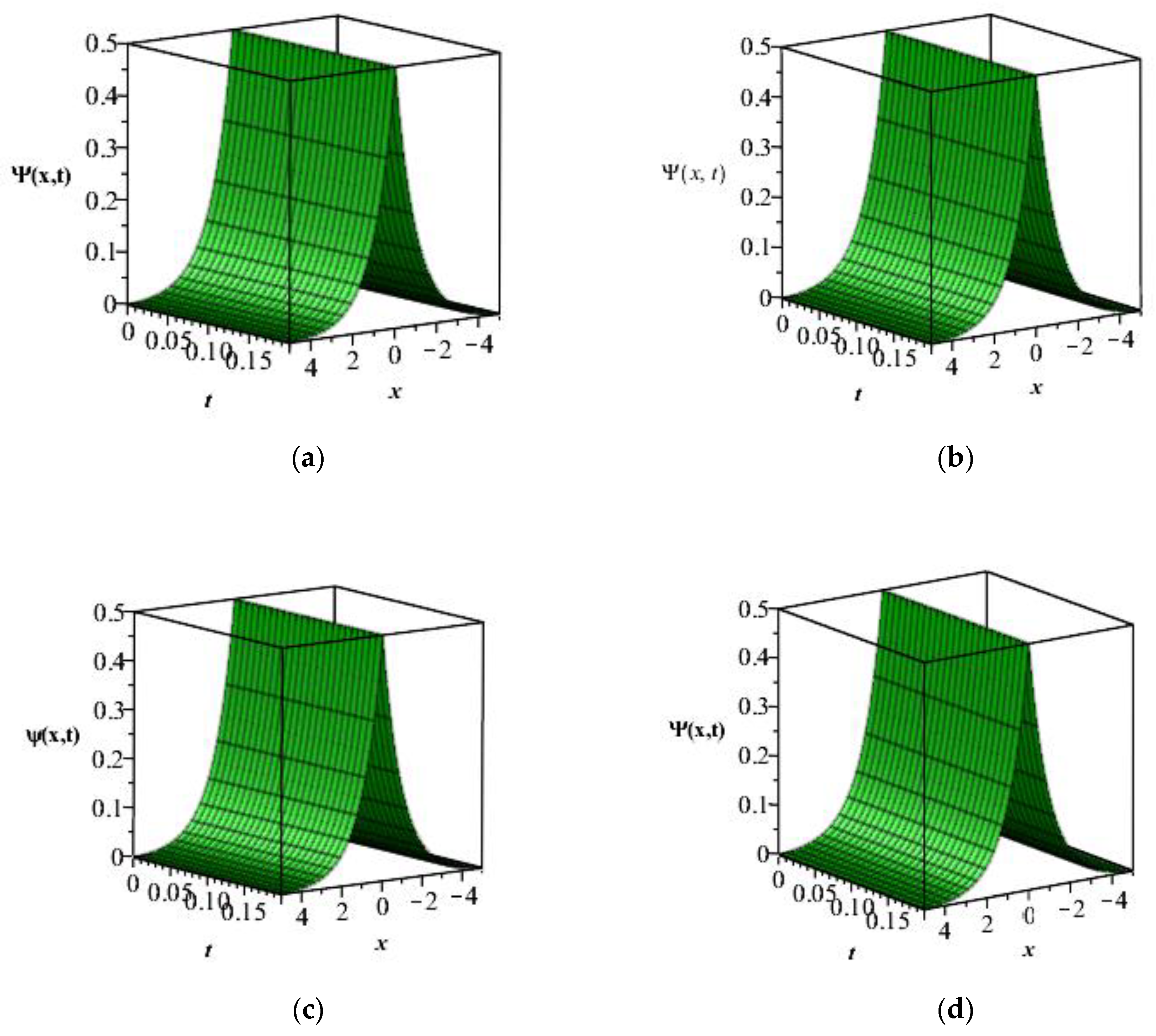
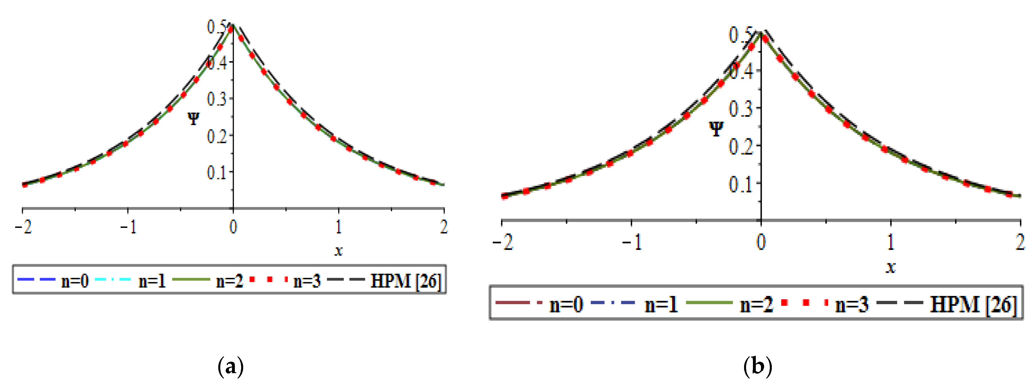
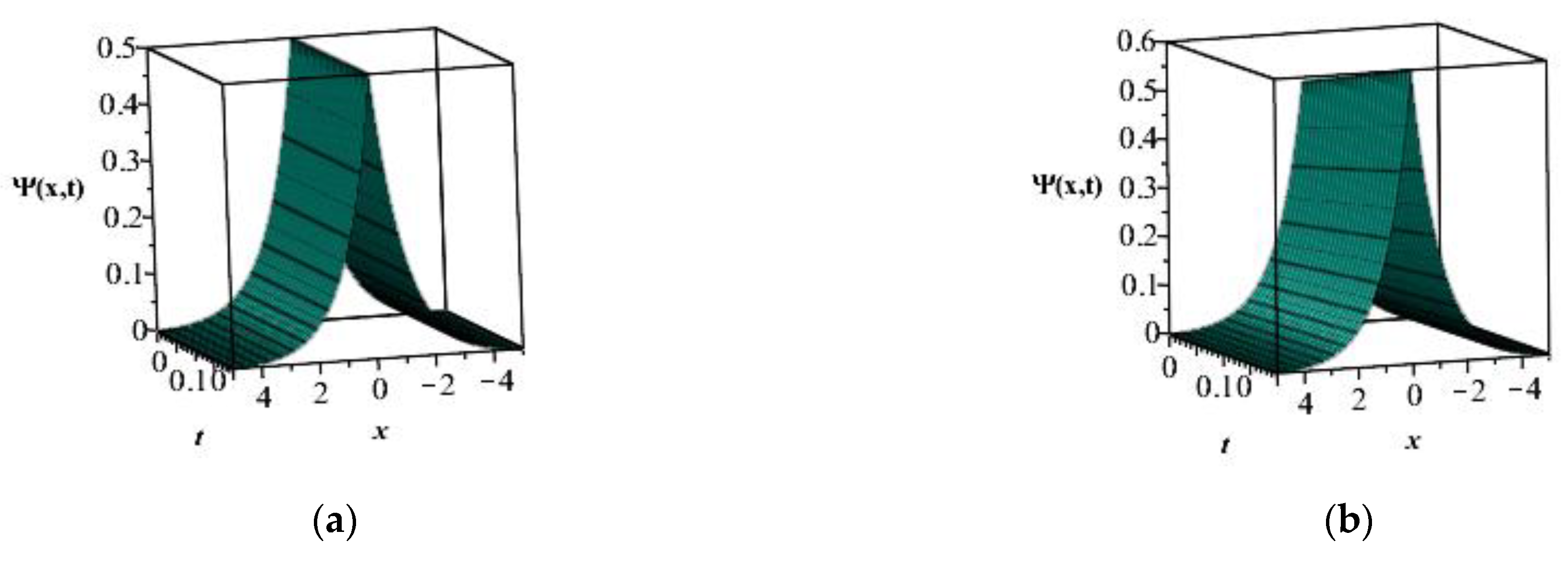
4. Implementation of FRDTM on the CH Equation

The time-fractional CH Equation (1) in an operator form as

$$D_t^{\alpha }\psi +2c\hspace{0.17em}{D}_x\psi -D_{xxt}\psi +3\psi \hspace{0.17em}{D}_x\psi =2D_x\psi \hspace{0.17em}{D}_{xx}\psi +\psi \hspace{0.17em}{D}_{xxx}\psi ,0<\alpha \le 1,$$

(20)

with IC

$$\psi \left(x,0\right)=g\left(x\right)$$

(21)

Applying FRDTM on Equations (20) and (21), the following recurrence relation is obtained as

$$\{\begin{array}{l}\frac{\mathsf{\Gamma }\left(1+\alpha k+\alpha \right)}{\mathsf{\Gamma }\left(1+\alpha k\right)}{\psi }_{k+1}\left(x\right)=2{\displaystyle \sum _{i=0}^k\left(\frac{\partial {\psi }_i\left(x\right)}{\partial x}\frac{{\partial }^2{\psi }_{k-i}\left(x\right)}{\partial x^2}\right)}+{\displaystyle \sum _{i=0}^k\left({\psi }_i\left(x\right)\frac{{\partial }^3{\psi }_{k-i}\left(x\right)}{\partial x^3}\right)-2c\frac{\partial {\psi }_k\left(x\right)}{\partial x}}+\frac{{\partial }^3{\psi }_k\left(x\right)}{\partial x^2\partial t}\\ -3{\displaystyle \sum _{i=0}^k\left({\psi }_i\left(x\right)\frac{\partial {\psi }_{k-i}\left(x\right)}{\partial x}\right)}\\ {\psi }_0\left(x\right)=g\left(x\right)\end{array}$$

(22)

Solving Equation (22) we obtain

$${\psi }_1\left(x\right)=\frac{1}{\mathsf{\Gamma }\left(1+\alpha \right)}\left(g\left(x\right)g^{\left(3\right)}\left(x\right)-2\left(c+\frac{3}{2}g\left(x\right)-g^{\left(2\right)}\left(x\right)\right)g^{\left(1\right)}\left(x\right)\right).$$

(23)

$${\psi }_2\left(x\right)=\frac{1}{\mathsf{\Gamma }\left(1+2\alpha \right)}\left[\begin{array}{l}{\left(g(x)\right)}^2{g}^{\left(6\right)}\left(x\right)+7g^{\left(1\right)}(x)g\left(x\right)g^{\left(5\right)}\left(x\right)+g^{\left(4\right)}\left(x\right)\\ \left(-4cg\left(x\right)-6g{\left(x\right)}^2+13g\left(x\right)g^{(2)}\left(x\right)+8{\left(g^{\left(1\right)}\left(x\right)\right)}^2\right)+8g\left(x\right){\left(g^{\left(3\right)}\left(x\right)\right)}^2\\ -12g^{\left(1\right)}\left(x\right){\left(g^{\left(3\right)}\left(x\right)\right)}^2\left(c+\frac{11}{4}g\left(x\right)-\frac{11}{6}{g}^{\left(2\right)}\left(x\right)\right)+4{\left(g^{\left(2\right)}\left(x\right)\right)}^3+\\ (-21g\left(x\right)-8c){\left(g^{\left(2\right)}(x)\right)}^2-30{\left(g^{\left(1\right)}\left(x\right)\right)}^2{g}^{\left(2\right)}\left(x\right)+4g^{\left(2\right)}\left(x\right){\left(c+\frac{3}{2}g\left(x\right)\right)}^2\\ +12{\left(g^{\left(1\right)}\left(x\right)\right)}^2\left(c+\frac{3}{2}g\left(x\right)\right)\end{array}\right].$$

(24)

Continuing the procedure, likewise, the rest of the components can be evaluated. So the approximate analytical solution of Equation (20) is

$$\psi \left(x,t\right)={\displaystyle \sum _{n=0}^{\infty }{\psi }_n\left(x\right)t^{n\alpha }}.$$

(25)

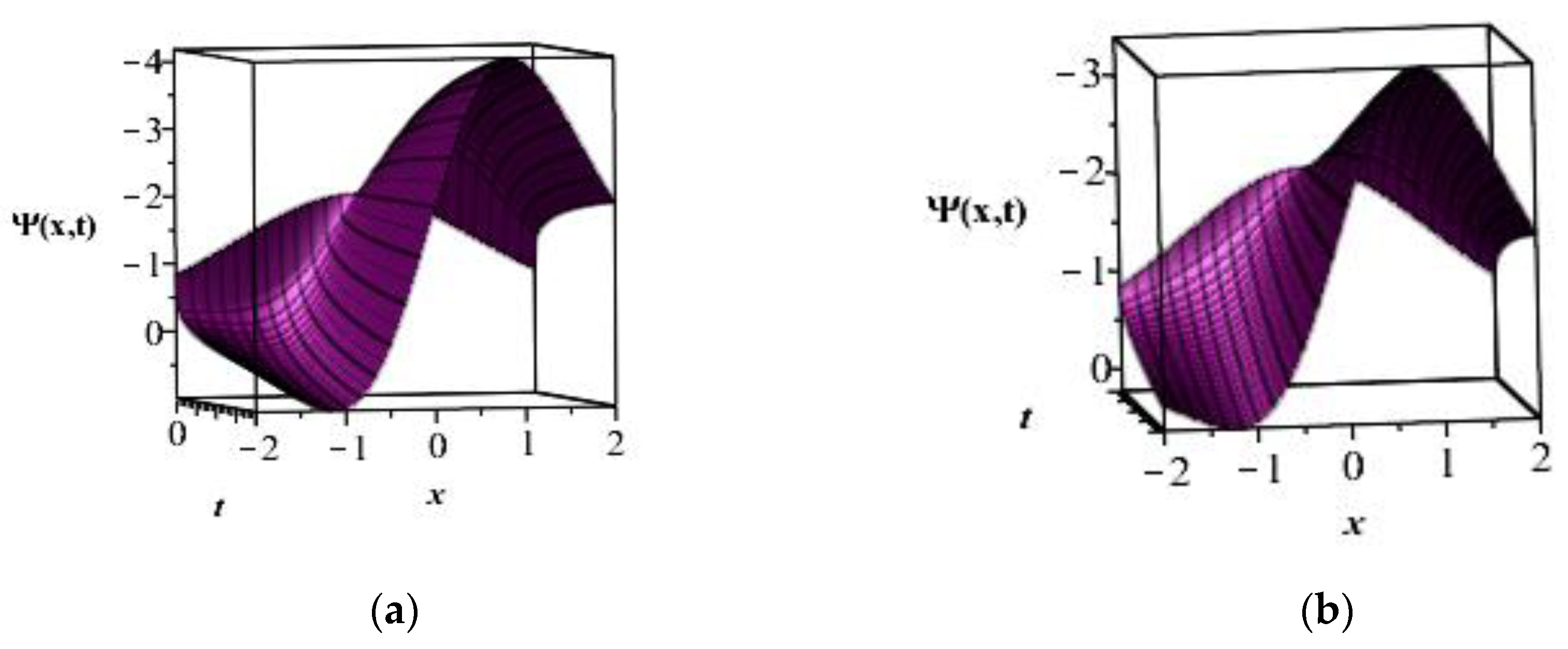
5. Implementation of FRDTM on the mCH Equation

Consider Equation (2) in an operator form as

$$D_t^{\alpha }\psi -D_{xxt}\psi +3{\psi }^2{D}_x\psi =2D_x\psi \hspace{0.17em}{D}_{xx}\psi +\psi \hspace{0.17em}{D}_{xxx}\psi$$

(26)

with IC

$$\psi \left(x,0\right)=p\left(x\right),$$

(27)

Using FRDTM on Equations (26) and (27), the following recurrence relation is obtained as

$$\{\begin{array}{l}\frac{\mathsf{\Gamma }\left(1+\alpha \hspace{0.17em}k+\alpha \right)}{\mathsf{\Gamma }\left(1+\alpha \hspace{0.17em}k\right)}{\psi }_{k+1}\left(x\right)=2{\displaystyle \sum _{i=0}^k\left(\frac{\partial {\psi }_i\left(x\right)}{\partial \hspace{0.17em}x}\frac{{\partial }^2{\psi }_{k-i}\left(x\right)}{\partial \hspace{0.17em}{x}^2}\right)}+{\displaystyle \sum _{i=0}^k\left({\psi }_i\frac{{\partial }^3{\psi }_{k-i}\left(x\right)}{\partial \hspace{0.17em}{x}^3}\right)+\frac{{\partial }^3{\psi }_k\left(x\right)}{\partial x^2\partial t}}\\ -3{\displaystyle \sum _{i=0}^k{\displaystyle \sum _{j=0}^i\left({\psi }_j{\psi }_{i-j}\frac{\partial {\psi }_{k-i}\left(x\right)}{\partial x}\right)}}\\ {\psi }_0\left(x\right)=p\left(x\right)\end{array}$$

(28)

Solving the recurrence relation Equation (28), we get

$${\psi }_1\left(x\right)=\frac{1}{\mathsf{\Gamma }\left(1+\alpha \right)}\left[p\left(x\right)p^{\left(3\right)}\left(x\right)-3{\left(p\left(x\right)\right)}^2{p}^{\left(1\right)}\left(x\right)+2p^{\left(2\right)}\left(x\right)p^{\left(1\right)}\left(x\right)\right].$$

(29)

$${\psi }_2\left(x\right)=\frac{1}{\mathsf{\Gamma }\left(1+2\alpha \right)}\left[\begin{array}{l}{\left(p(x)\right)}^2{p}^{\left(6\right)}\left(x\right)+7p^{\left(1\right)}(x)p\left(x\right)p^{\left(5\right)}\left(x\right)+p^{\left(4\right)}\left(x\right)\\ \left(-6{(p\left(x\right))}^3+13p\left(x\right)p^{(2)}\left(x\right)+8{\left(p^{\left(1\right)}\left(x\right)\right)}^2\right)+8p\left(x\right){\left(p^{\left(3\right)}\left(x\right)\right)}^2\\ -48p^{\left(1\right)}\left(x\right){\left(p^{\left(3\right)}\left(x\right)\right)}^2\left({\left(p\left(x\right)\right)}^2-\frac{11}{24}{p}^{\left(2\right)}\left(x\right)\right)+4{\left(p^{\left(2\right)}\left(x\right)\right)}^3+\\ (-30p\left(x\right)){\left(p^{\left(2\right)}(x)\right)}^2+9{\left(p\left(x\right)\right)}^2{p}^{\left(2\right)}\left(x\right)-96p\left(x\right){\left(p^{(1)}\left(x\right)\right)}^2{p}^{\left(2\right)}\left(x\right)\\ +36{\left(p\left(x\right)\right)}^3{\left(p^{\left(1\right)}\left(x\right)\right)}^2-12{\left(p^{\left(1\right)}\left(x\right)\right)}^4\end{array}\right]$$

(30)

Similarly, the rest of the components ${\psi }_3,{\psi }_4,\dots$ can be evaluated. So the approximate analytical solution of Equation (26) is

$$\psi \left(x,t\right)={\displaystyle \sum _{n=0}^{\infty }{\psi }_n\left(x\right)t^{n\alpha }},$$

(31)

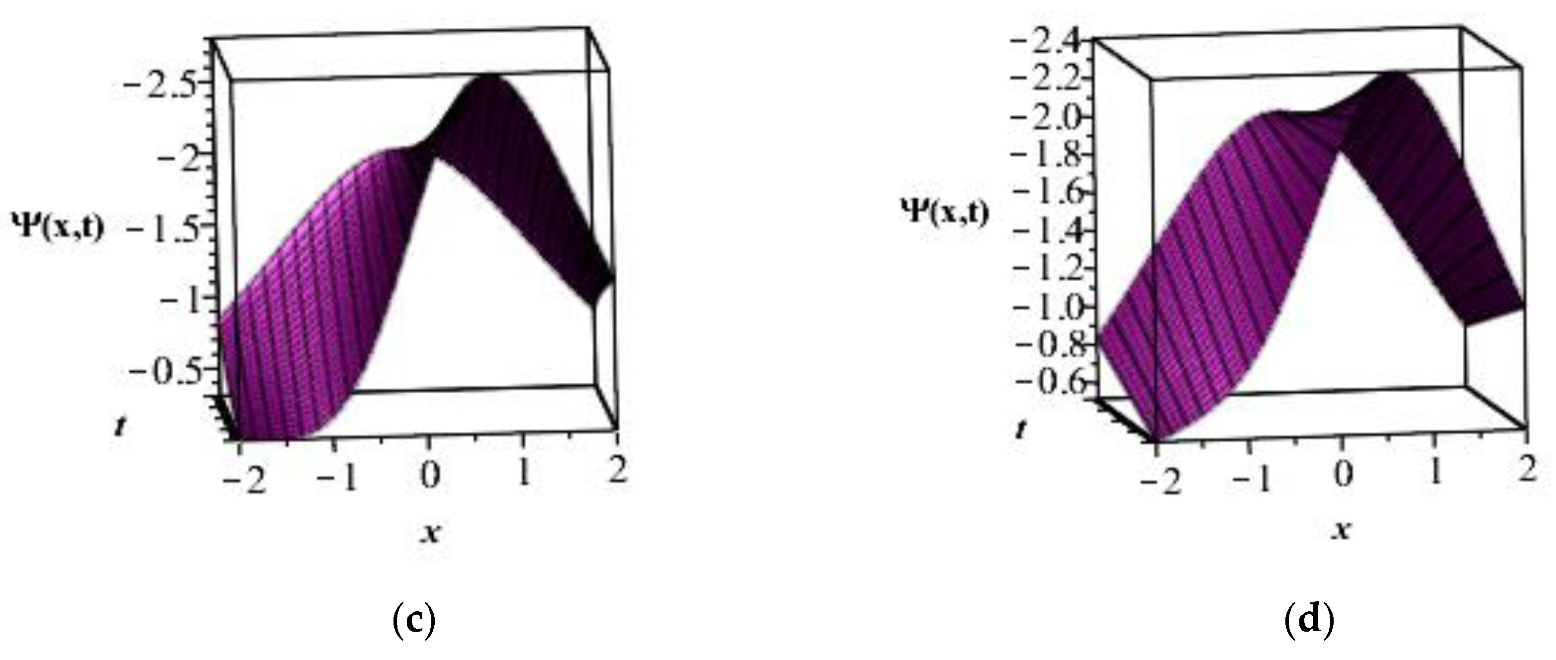
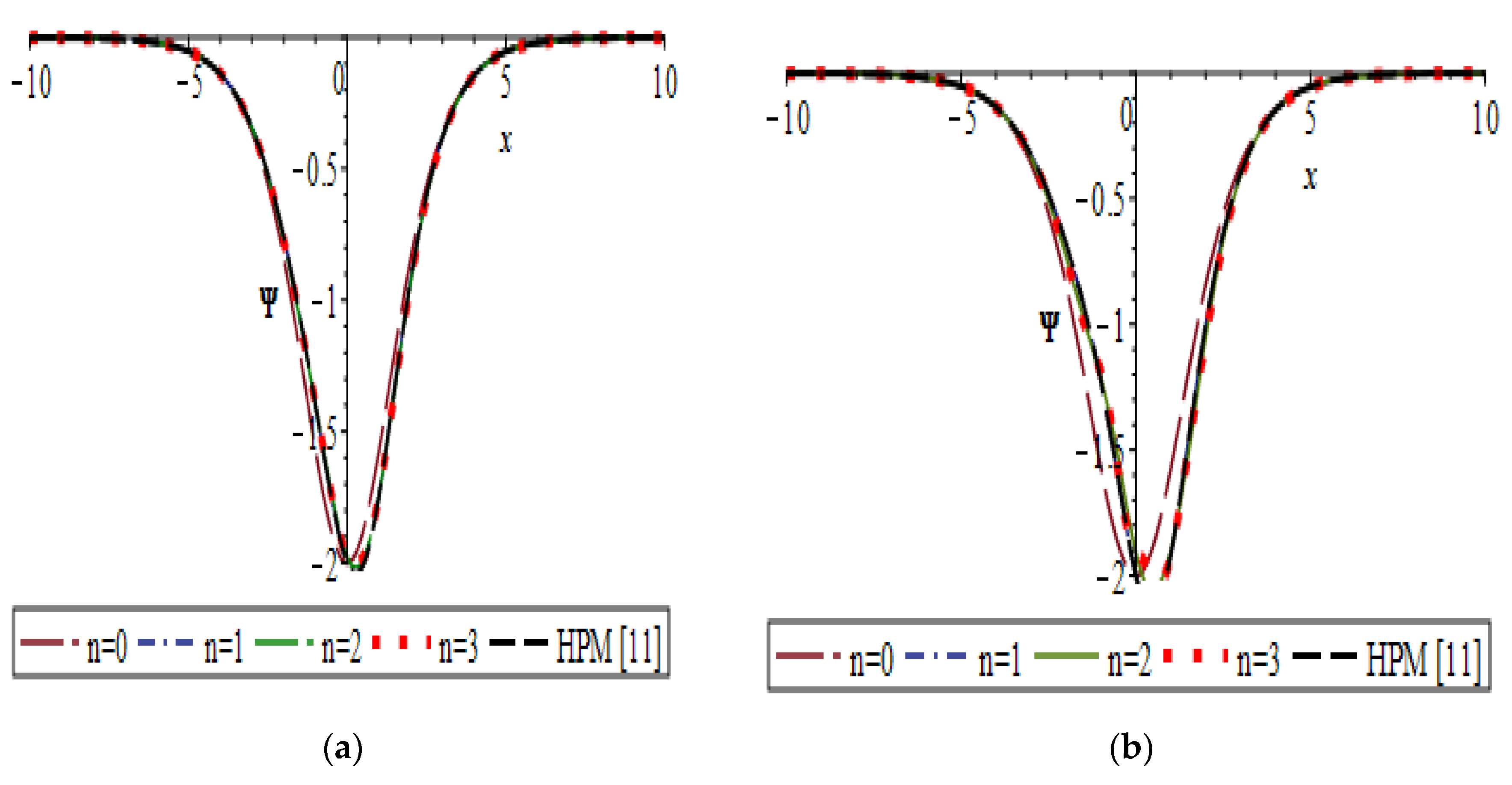
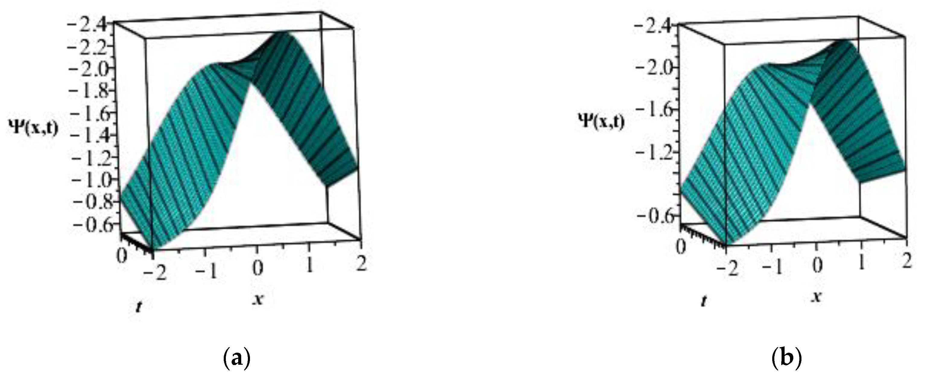
6. Implementation of FRDTM on the DP Equation

Considering Equation (3) in operator form, we get

$$D_t^{\alpha }\psi -D_{xxt}\psi +4{\psi }^2{D}_x\psi =3D_x\psi \hspace{0.17em}{D}_{xx}\psi +\psi \hspace{0.17em}{D}_{xxx}\psi ,$$

(32)

with IC

$$\psi \left(x,0\right)=f\left(x\right)$$

(33)

Applying FRDTM to Equation (32), we obtain

$$\{\begin{array}{l}\frac{\mathsf{\Gamma }\left(1+\alpha \hspace{0.17em}k+\alpha \right)}{\mathsf{\Gamma }\left(1+\alpha \hspace{0.17em}k\right)}{\psi }_{k+1}\left(x\right)=3{\displaystyle \sum _{i=0}^k\left(\frac{\partial {\psi }_i\left(x\right)}{\partial \hspace{0.17em}x}\frac{{\partial }^2{\psi }_{k-i}\left(x\right)}{\partial \hspace{0.17em}{x}^2}\right)}+{\displaystyle \sum _{i=0}^k\left({\psi }_i\frac{{\partial }^3{\psi }_{k-i}\left(x\right)}{\partial \hspace{0.17em}{x}^3}\right)+\frac{{\partial }^3{\psi }_k\left(x\right)}{\partial \hspace{0.17em}{x}^2\partial \hspace{0.17em}t}}\\ -4{\displaystyle \sum _{i=0}^k{\displaystyle \sum _{j=0}^i\left({\psi }_j{\psi }_{i-j}\frac{\partial {\psi }_{k-i}\left(x\right)}{\partial \hspace{0.17em}x}\right)}}\end{array}$$

(34)

Applying FRDTM to Equation (33), we get

$${\psi }_0\left(x\right)=f\left(x\right).$$

(35)

Substituting Equation (35) in Equation (34), the following recursive values of ${\left({\psi }_n\right)}_{n=1}^{\infty }$ are obtained

$${\psi }_1\left(x\right)=\frac{1}{\mathsf{\Gamma }\left(1+\alpha \right)}\left[f\left(x\right)f^{\left(3\right)}\left(x\right)-4{\left(p\left(x\right)\right)}^2{p}^{\left(1\right)}\left(x\right)+3p^{\left(2\right)}\left(x\right)p^{\left(1\right)}\left(x\right)\right].$$

(36)

$${\psi }_2\left(x\right)=\frac{1}{\mathsf{\Gamma }\left(1+2\alpha \right)}\left[\begin{array}{l}{\left(f(x)\right)}^2{f}^{\left(6\right)}\left(x\right)+9f^{\left(1\right)}(x)f\left(x\right)f^{\left(5\right)}\left(x\right)+f^{\left(4\right)}\left(x\right)\\ \left(-8{(f\left(x\right))}^3+18f\left(x\right)f^{(2)}\left(x\right)+15{\left(f^{\left(1\right)}\left(x\right)\right)}^2\right)+11f\left(x\right){\left(f^{\left(3\right)}\left(x\right)\right)}^2\\ -72f^{\left(1\right)}\left(x\right)\left(f^{\left(3\right)}\left(x\right)\right)\left({\left(f\left(x\right)\right)}^2-\frac{5}{8}{f}^{\left(2\right)}\left(x\right)\right)+9{\left(f^{\left(2\right)}\left(x\right)\right)}^3\\ -48{\left(f\left(x\right)\right)}^2{\left(f^{\left(2\right)}(x)\right)}^2+16{\left(f\left(x\right)\right)}^4{f}^{\left(2\right)}\left(x\right)-168f\left(x\right){\left(f^{(1)}\left(x\right)\right)}^2{f}^{\left(2\right)}\left(x\right)\\ +64{\left(f\left(x\right)\right)}^3{\left(f^{\left(1\right)}\left(x\right)\right)}^2-24{\left(f^{\left(1\right)}\left(x\right)\right)}^4\end{array}\right].$$

(37)

Continuing in this manner ${\psi }_3,{\psi }_4,\dots$ can be evaluated. So the approximate analytical solution of Equation (32) is

$$\psi \left(x,t\right)={\displaystyle \sum _{n=0}^{\infty }{\psi }_n\left(x\right)t^{n\alpha }}$$

(38)

7. Results and Discussion

In this section, approximate solutions of displacement $\psi \left(x,t\right)\hspace{0.17em}$ for different values of $\alpha$ are calculated for different values of $t$ and $x$ at fixed $c=0.005$ and $k=0.5$. In Section 4, IC [24,28] is considered as $\psi \left(x,0\right)=g\left(x\right)=\left(k+c\right)e^{-\left|x\right|}-c$ for showing the nature of the displacements of CH Equation (1). The solutions $\psi \left(x,t\right)\hspace{0.17em}$ for different values of $t$, $x$ and $\alpha$ are depicted in Figure 1a–d for the CH equation. In Section 5, we considered the IC [11] as $\psi \left(x,0\right)=p\left(x\right)=-2{\mathrm{sech}}^2\left(\frac{x}{2}\right)$, a particular case for viewing the behavior of the displacements. The numerical results of $\psi \left(x,t\right)\hspace{0.17em}$ for various values of $t$, $x$ and $\alpha$ are portrayed in Figure 2a–d for the mCH Equation (2). Similarly, in Section 6, the IC [11] is assumed as $\psi \left(x,0\right)=f\left(x\right)=-\frac{15}{8}{\mathrm{sech}}^2\left(\frac{x}{2}\right)$ for presenting the nature of the displacements. The numerical solutions $\psi \left(x,t\right)\hspace{0.17em}$ for various values of $t$, $x$ and $\alpha$ are illustrated in Figure 3a–d for the DP Equation (3). Also, comparison tests have been included among the existing solution and the results of Zhang et al. [11] and Zhang et al. [28] in Figure 4, Figure 5, Figure 6, Figure 7, Figure 8 and Figure 9. One may see from

Table 2. The two term FRDTM approximation results of CH equation with HPM [28] for $\alpha =1$.

$\left(\mathit{x},\mathit{t}\right)$	${\mathit{\psi }}_{\mathit{H}\mathit{P}\mathit{M}}$ [28]	FRDTM (n = 0)	FRDTM (n = 1)	FRDTM (n = 2)	FRDTM (n = 3)
(0.1, 0.05)	0.47479025	0.45194289	0.45194289	0.45194289	0.45194289
(0.2, 0.05)	0.42913217	0.40845903	0.40845903	0.40845903	0.40845903
(0.4, 0.05)	0.35043736	0.33351162	0.33351162	0.33351162	0.33351162
(0.8, 0.05)	0.23325678	0.22191112	0.22191112	0.22191112	0.22191112
(−0.2, 0.05)	0.42913217	0.40845903	0.40845903	0.40845903	0.40845903
(−0.4, 0.05)	0.35043736	0.33351162	0.33351162	0.33351162	0.33351162
CPU time		0.053s	0.063s	0.078s	0.124s

,

Table 3. The two term FRDTM approximation results of mCH equation with HPM [11] for $\alpha =1$

$\left(\mathit{x},\mathit{t}\right)$	${\mathit{\psi }}_{\mathit{H}\mathit{P}\mathit{M}}$ [11]	FRDTM (n = 0)	FRDTM (n = 1)	FRDTM (n = 2)	FRDTM (n = 3)
(8, 0.05)	−0.00268298	−0.00268190	−0.00268297	−0.00268298	−0.00268298
(9, 0.05)	−0.00098718	−0.00098703	−0.00098718	−0.00098718	−0.00098718
(10, 0.05)	−0.00036318	−0.00036316	−0.00036318	−0.00036318	−0.00036318
(8, 0.1)	−0.00268406	−0.00268105	−0.00268405	−0.00268406	−0.00268406
(9, 0.1)	−0.00098732	−0.00098703	−0.00098732	−0.00098732	−0.00098732
(10, 0.1)	−0.00036320	−0.00036316	−0.00036320	−0.00036320	−0.00036320
CPU time		0.063 s	0.093 s	0.078 s	0.094 s

and

Table 4. The two term FRDTM approximation results of DP equation with HPM [11] for $\alpha =1$

$\left(\mathit{x},\mathit{t}\right)$	${\mathit{\psi }}_{\mathit{H}\mathit{P}\mathit{M}}$ [11]	FRDTM (n = 0)	FRDTM (n = 1)	FRDTM (n = 2)	FRDTM (n = 3)
(0, 0)	−1.875	−1.8750	−1.875	−1.875	−1.875
(0.2, 0.2)	−2.1311490	−1.8563742	−2.1311490	−2.1311490	−2.1311490
(0.4, 0.4)	−2.8273737	−1.8019555	−2.8273737	−2.8273737	−2.8273737
(0.8, 0.8)	−4.7337056	−4.7337056	−4.7337056	−4.7337056	−4.7337056
(−0.2, 0.2)	−1.5815995	−1.8563742	−1.5815995	−1.5815995	−1.5815995
(−0.4, 0.4)	−0.7765374	−1.8019555	−0.7765374	−0.7765374	−0.7765374
CPU time		0.01 s	0.016 s	0.062 s	0.078 s

that approximate solutions solved by FRDTM are quite close to the solutions solved by Zhang et al. [11,28].

8. Conclusions

In this article, FRDTM is successfully implemented for solving time-fractional CH, mCH, and DP equations with suitable initial conditions. Solutions are obtained without any transformation and perturbation. Three test problems were performed to validate the precision and efficacy of the current method. Also, it was seen that the obtained results are a good agreement with the solution obtained by Zhang et al. [11,28]. The main benefit of this approach is that linearization is not required for this method and therefore it reduces complex numerical computations significantly compared to the other existing methods such as the perturbation technique, DTM, and ADM. Small size computations over other techniques are the main advantages of the proposed method.

References

1. Podlubny, I. Fractional Differential Equations; Academic Press: San Diego, CA, USA, 1999. [Google Scholar]
2. Miller, K.S.; Ross, B. An Introduction to the Fractional Calculus and Fractional Differential Equations; Wiley: New York, NY, USA, 1993. [Google Scholar]
3. Caputo, M.; Mainardi, F. Linear models of dissipation in an elastic solids. Riv. Nuovo Cim. 1971, 1, 161–198. [Google Scholar] [CrossRef]
4. Carpinteri, A.; Mainardi, F. Fractals and Fractional Calculus in Continuum Mechanics; Springer: New York, NY, USA, 1997. [Google Scholar]
5. Jena, R.M.; Chakraverty, S. A new iterative method based solution for fractional Black–Scholes option pricing equations (BSOPE). SN Appl. Sci. 2019, 1, 95. [Google Scholar] [CrossRef]
6. Baleanu, D.; Diethelm, K.; Scalas, E.; Trujillo, J.J. Fractional Calculus: Models and Numerical Methods; World Scientific Publishing Company: Boston, MA, USA, 2012. [Google Scholar]
7. Baleanu, D.; Machado, J.A.T.; Luo, A.C. Fractional Dynamics and Control; Springer: Berlin, Germany, 2012. [Google Scholar]
8. Jena, R.M.; Chakraverty, S. Residual power series method for solving time-fractional model of vibration equation of large membranes. J. Appl. Comput. Mech. 2019, 5, 603–615. [Google Scholar]
9. He, J.H. Nonlinear oscillation with fractional derivative and its applications. Int. Conf. Vib. Eng. 1998, 98, 288–291. [Google Scholar]
10. Javeed, S.; Baleanu, D.; Waheed, A.; Khan, M.S.; Affan, H. Analysis of Homotopy Perturbation Method for Solving Fractional Order Differential Equations. Mathematics 2019, 7, 40. [Google Scholar] [CrossRef]
11. Zhang, B.G.; Li, S.Y.; Liu, Z.R. Homotopy perturbation method for modified Camassa-Holm and Degasperis-Procesi equations. Phys. Lett. A 2008, 372, 1867–1872. [Google Scholar] [CrossRef]
12. Jena, R.M.; Chakraverty, S. Solving time-fractional Navier–Stokes equations using homotopy perturbation Elzaki transform. SN Appl. Sci 2019, 1, 16. [Google Scholar] [CrossRef]
13. Singh, J.; Kumar, D.; Kilicman, A. Numerical solutions of nonlinear fractional partial differential equations arising in spatial diffusion of biological populations. Abstr. Appl. Anal. 2014, 535793. [Google Scholar] [CrossRef]
14. Jena, R.M.; Chakraverty, S.; Jena, S.K. Dynamic Response Analysis of Fractionally Damped Beams Subjected to External Loads using Homotopy Analysis Method. J. Appl. Comput. Mech. 2019, 5, 355–366. [Google Scholar]
15. Ganji, Z.Z.; Ganji, D.D.; Ganji, A.D.; Rostamian, M. Analytical solution of time-fractional Navier–Stokes equation in polar coordinate by homotopy perturbation method. Numer. Methods Part Differ. Equ. 2010, 26, 117–124. [Google Scholar] [CrossRef]
16. Yavuz, M.; Ozdemir, N. A Quantitative Approach to Fractional Option Pricing Problems with Decomposition Series. Konuralp J. Math. 2018, 6, 102–109. [Google Scholar]
17. Edeki, S.O.; Motsepa, T.; Khalique, C.M.; Akinlabi, G.O. The Greek parameters of a continuous arithmetic Asian option pricing model via Laplace Adomian decomposition method. Open Phys. 2018, 16, 780–785. [Google Scholar] [CrossRef]
18. Wazwaz, A.M. Solitary wave solutions for modified forms of Degasperis-Procesi and Camassa-Holm equations. Phys. Lett. A 2006, 352, 500–504. [Google Scholar] [CrossRef]
19. Jena, R.M.; Chakraverty, S. Analytical solution of Bagley-Torvik equations using Sumudu transformation method. SN Appl. Sci. 2019, 1, 246. [Google Scholar] [CrossRef] [Green Version]
20. Kumar, D.; Singh, J.; Kumar, S. Numerical computation of fractional multi-dimensional diffusion equations by using a modified homotopy perturbation method. J. Assoc. Arab Univ. Basic Appl. Sci 2014, 17, 20–26. [Google Scholar] [CrossRef]
21. Odibat, Z.; Momani, S. Modified homotopy perturbation method application to quadratic Riccati differential equation of fractional order. Chaos Solitons Fractals 2008, 36, 167–174. [Google Scholar] [CrossRef]
22. Keskin, Y.; Oturanc, G. Reduced differential transform method: a new approach to fractional partial differential equations. Nonlinear Sci. Lett. A 2010, 1, 61–72. [Google Scholar]
23. Camassa, R.; Holm, D.D. An integrable shallow water equation with peaked solitons. Phys. Rev. Lett. 1993, 71, 1661–1664. [Google Scholar] [CrossRef] [Green Version]
24. Gupta, P.K.; Singh, M.; Yildirim, A. Approximate analytical solution of the time fractional Camassa-Holm, modified Camassa-Holm, and Degasperis-Procesi equations by homotopy perturbation method. Sci. Iran. A 2016, 23, 155–165. [Google Scholar]
25. Ganji, D.D.; Sadeghi, E.M.M.; Rahmat, M.G. Modified Camassa–Holm and Degasperis–Procesi Equations Solved by Adomian’s Decomposition Method and Comparison with HPM and Exact Solutions. Acta Appl. Math. 2008, 104, 303–311. [Google Scholar] [CrossRef]
26. Lundmark, H.; Szmigielski, J. Multi-peakon solutions of the Degasperis–Procesi equation. Inverse Probl. 2003, 19, 1241–1245. [Google Scholar] [CrossRef]
27. Degasperis, A.; Procesi, M. Asymptotic Integrability Symmetry and Perturbation Theory; World Scientific: Singapore, 2002; pp. 23–27. [Google Scholar]
28. Zhang, B.G.; Li, S.Y.; Mao, J.F. Approximate explicit solution of Camassa-Holm equation by He’s homotopy perturbation method. J. Appl. Math. Comput. 2009, 31, 239–246. [Google Scholar] [CrossRef]
Figure 1. The solution plots of ψ ( x , t ) at (a) α = 0.5 (b) α = 0.25 (c) α = 0.75 (d) α = 1 with c = 0.005 and k = 0.5 for Equation (25).
Mathematics 07 00722 g001
Figure 2. Plots of ψ ( x , t ) with respect to x and t at (a) α = 0.5 (b) α = 0.25 (c) α = 0.75 (d) α = 1 for Equation (31).
Mathematics 07 00722 g002aMathematics 07 00722 g002b
Figure 3. Plots of ψ ( x , t ) with respect to x and t at (a) α = 0.5 (b) α = 0.25 (c) α = 0.75 (d) α = 1 for Equation (38).
Mathematics 07 00722 g003
Figure 4. Comparison plots of ψ F R D T M and ψ H P M of Camassa–Holm (CH) equation for 2 x 2 . (a) c = 0.005 , k = 0.5 , t = 0.05 , α = 1 ; (b) c = 0.005 , k = 0.5 , t = 0.1 , α = 1 .
Mathematics 07 00722 g004
Figure 5. The solution plots of CH equation at α = 1 (a) two-terms FRDTM solution (b) homotopy perturbation method (HPM) solution [28].
Mathematics 07 00722 g005
Figure 6. Comparison plots of ψ F R D T M and ψ H P M of modified Camassa–Holm (mCH) equation for 10 x 10 . (a) t = 0.05 , α = 1 ; (b) t = 0.1 , α = 1 .
Mathematics 07 00722 g006
Figure 7. The solution plots of mCH equation at α = 1 (a) two-terms FRDTM solution (b) HPM solution [11].
Mathematics 07 00722 g007
Figure 8. Comparison plots of ψ F R D T M and ψ H P M [11] of Degasperis–Procesi (DP) equation for 10 x 10 . (a) t = 0.05 , α = 1 ; (b) t = 0.1 , α = 1 .
Mathematics 07 00722 g008
Figure 9. The solution plots of DP equation at α = 1 . (a) two-terms FRDTM solution (b) HPM solution [11].
Mathematics 07 00722 g009