The Regularity of Some Families of Circulant Graphs

Abstract

We compute the Castelnuovo–Mumford regularity of the edge ideals of two families of circulant graphs, which includes all cubic circulant graphs. A feature of our approach is to combine bounds on the regularity, the projective dimension, and the reduced Euler characteristic to derive an exact value for the regularity.

1. Introduction

Let G be any finite simple graph with vertex set $V(G)=\{x_1,\dots ,x_n\}$ and edge set $E(G)$, where simple means no loops or multiple edges. The edge ideal of G is the ideal $I(G)=〈x_i{x}_j\mid \{x_i,x_j\}\in E(G)〉$ in $R=k[x_1,\dots ,x_n]$, a standard graded polynomial ring over a field k (k is any field). Describing the dictionary between the graph theoretic properties of G and the algebraic properties of $I(G)$ or $R/I(G)$ is an active area of research; e.g., see [1,2].

Relating the homological invariants of $I(G)$ and the graph theoretic invariants of G has proven to be a fruitful approach to building this dictionary. Recall that the minimal graded free resolution of $I(G)\subseteq R$ is a long exact sequence of the form:

$$0\to \underset{j}{⨁}R{(-j)}^{{\beta }_{l,j}(I(G))}\to \underset{j}{⨁}R{(-j)}^{{\beta }_{l-1,j}(I(G))}\to \cdots \to \underset{j}{⨁}R{(-j)}^{{\beta }_{0,j}(I(G))}\to I(G)\to 0$$

where $l\le n$. Here, $R(-j)$ denotes the free R-module obtained by shifting the degrees of R by j, that is $R{(-j)}_a=R_{a-j}$. We denote by ${\beta }_{i,j}(I(G))$ the $i,j^{\mathrm{th}}$ graded Betti number of $I(G)$; this number equals the number of minimal generators of degree j in the $i^{\mathrm{th}}$ syzygy module of $I(G)$. Two invariants that measure the “size” of the resolution are the (Castelnuovo–Mumford) regularity and the projective dimension, defined as:

$$\begin{array}{ccc}\hfill \mathrm{reg}(I(G))& =& max\{j-i\mid {\beta }_{i,j}(I(G))\ne 0\},\mathrm{and}\hfill \\ \hfill \mathrm{pd}(I(G))& =& max\{i\mid {\beta }_{i,j}(I(G))\ne 0\mathrm{for}\mathrm{some}j\}.\hfill \end{array}$$

One wishes to relate the numbers ${\beta }_{i,j}(I(G))$ to the invariants of G; e.g., see the survey of Hà [3], which focuses on describing $\mathrm{reg}(I(G))$ in terms of the invariants of G.

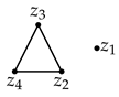
In this note, we give explicit formulas for $\mathrm{reg}(I(G))$ for the edge ideals of two infinite families of circulant graphs. Our results complement previous work on the algebraic and combinatorial topological properties of circulant graphs (e.g, [4,5,6,7,8,9,10,11]). Fix an integer $n\ge 2$ and a subset $S\subseteq \{1,\dots ,\lfloor \frac{n}{2}\rfloor \}$. The circulant graph $C_n(S)$ is the graph on the vertex set $\{x_1,\dots ,x_n\}$ such that $\{x_i,x_j\}\in E(C_n(S))$ if and only if $|i-j|$ or $n-|i-j|\in S$. To simplify notation, $C_n(a_1,\dots ,a_t)$ is sometimes written for $C_n(\{a_1,\dots ,a_t\})$. 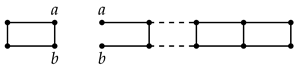As an example, the graph $C_{10}(1,3)$ is drawn in Figure 1.

When $S=\{1,\dots ,\lfloor \frac{n}{2}\rfloor \}$, then $C_n(S)\cong K_n$, the clique on n vertices. On the other hand, if $S=\left\{1\right\}$, then $C_n(1)\cong C_n$, the cycle on n vertices. For both of these families, the regularity of their edge ideals is known. Specifically, the ideal $I(K_n)$ has a linear resolution by Fröberg’s theorem [12], so $\mathrm{reg}(I(K_n))=2$. The value of $\mathrm{reg}(I(C_n))$ can be deduced from the work of Jacques ([13], Theorem 7.6.28). One can view these circulant graphs as “extremal” cases in the sense that $\left|S\right|$ is either as large or as small as possible.

Our motivation is to understand the next open cases. In particular, generalizing the case of $K_n$, we compute $\mathrm{reg}(I(C_n(S))$ when $S=\{1,\dots ,\widehat{j},\dots ,\lfloor \frac{n}{2}\rfloor \}$ for any $1\le j\le \lfloor \frac{n}{2}\rfloor$ (Theorem 5). For most j, the regularity follows from Fröberg’s theorem and a result of Nevo [14]. To generalize the case of $C_n$ (a circulant graph where every vertex has degree two), we compute the regularity of the edge ideal of any cubic (every vertex has degree three) circulant graph, that is $G=C_{2n}(a,n)$ with $1\le a\le n$ (Theorem 8). Our proof of Theorem 8 requires a new technique to compute $\mathrm{reg}(I)$ for a square-free monomial ideal. Specifically, we show how to use partial information about $\mathrm{reg}(I)$, $\mathrm{pd}(I)$, and the reduced Euler characteristic of the simplicial complex associated with I to determine $\mathrm{reg}(I)$ exactly (see Theorem 4). We believe this result to be of independent interest.

We use the following outline. We first recall the relevant background regarding graph theory and commutative algebra, along with our new result on the regularity of square-free monomial ideals. In Section 3, we compute the regularity of $I(G)$ for the family of graphs $G=C_n(1,\dots ,\widehat{j},\dots ,\lfloor \frac{n}{2}\rfloor )$. In Section 4, we give an explicit formula for the regularity of edge ideals of cubic circulant graphs.

2. Background

We review the relevant background from graph theory and commutative algebra. In addition, we give a new result on the regularity of square-free monomial ideals.

2.1. Graph Theory Preliminaries

Let $G=(V(G),E(G))$ denote a finite simple graph. We abuse notation and write $xy$ for the edge $\{x,y\}\in E(G)$. The complement of G, denoted $G^c$, is the graph $(V(G^c),E(G^c))$ where $V(G^c)=V(G)$ and $E(G^c)=\left\{xy\right|xy\notin E(G)\}$. The neighbours of $x\in V(G)$ are the set $N(x)=\{y\in V(G)|xy\in E(G)\}$. The closed neighbourhood of x is $N\left[x\right]=N(x)\cup \left\{x\right\}$. The degree of x is $deg(x)=|N(x)|$. If we need to highlight the graph, we write $N_G\left[x\right]$ or $N_G(x)$.

A graph $H=(V(H),E(H))$ is a subgraph of G if $V(H)\subseteq V(G)$ and $E(H)\subseteq E(G)$. Given a subset $W\subseteq V(G)$, the induced subgraph of G on W is the graph $G_W=(W,E(G_W))$ where $E(G_W)=\{xy\in E(G)|\{x,y\}\subseteq W\}$. Notice that an induced subgraph is a subgraph of G, but not every subgraph of G is an induced subgraph.

An n-cycle, denoted $C_n$, is the graph with $V(C_n)=\{x_1,\dots ,x_n\}$ and edges $E(C_n)=\{x_1{x}_2,x_2{x}_3,\dots ,x_{n-1}{x}_n,x_n{x}_1\}$. A graph G has a cycle of length n if G has a subgraph of the form $C_n$. A graph is a chordal graph if G has no induced graph of the form $C_n$ with $n\ge 4$. A graph G is co-chordal if $G^c$ is chordal. The co-chordal number of G, denoted $\mathrm{co}\text{-}\mathrm{chord}(G)$, is the smallest number of subgraphs of G such that $G=G_1\cup \cdots \cup G_s$, and each $G_i^c$ is a chordal graph.

A claw is the graph with $V(G)=\{x_1,x_2,x_3,x_4\}$ with edges $E(G)=\{x_1{x}_2,x_1{x}_3,x_1{x}_4\}$. A graph is claw-free if no induced subgraph of the graph is a claw. A graph G is gap-free if no induced subgraph of $G^c$ is a $C_4$. Finally, the complete graph $K_n$ is the graph with $V(K_n)=\{x_1,\dots ,x_n\}$ and $E(K_n)=\left\{x_i{x}_j\right|1\le i<j\le n\}$.

2.2. Algebraic Preliminaries

We recall some facts about the regularity of $I(G)$. Note that for any homogeneous ideal, $\mathrm{reg}(I)=\mathrm{reg}(R/I)+1$.

We collect together a number of useful results on the regularity of edge ideals.

Theorem 1.

Let G be a finite simple graph. Then:

(i)

if $G=H\cup K$, with H and K disjoint, then:

$$\mathrm{reg}(R/I(G))=\mathrm{reg}(R/I(H))+\mathrm{reg}(R/I(K)).$$

(ii)

$\mathrm{reg}(I(G))=2$ if and only if $G^c$ is a chordal graph.

(iii)

$\mathrm{reg}(I(G))\le \mathrm{co}\text{-}\mathrm{chord}(G)+1$.

(iv)

if G is gap-free and claw-free, then $\mathrm{reg}(I(G))\le 3$.

(v)

if $x\in V(G)$, then $\mathrm{reg}(I(G))\in \{\mathrm{reg}(I(G\setminus N_G\left[x\right]))+1,\mathrm{reg}(I(G\setminus x))\}.$

Proof. 

For $(i)$, see Woodroofe ([15], Lemma 8). Statement $(ii)$ is Fröberg’s Theorem ([12], Theorem 1). Woodroofe ([15], Theorem 1) first proved $(iii)$. Nevo first proved $(iv)$ in [14] (Theorem 5.1). For $(v)$, see Dao, Huneke, and Schweig ([16], Lemma 3.1). ☐

We require a result of Kalai and Meshulam [17] that has been specialized to edge ideals.

Theorem 2. 

([17], Theorems 1.4 and 1.5) Let G be a finite simple graph, and suppose H and K are subgraphs such that $G=H\cup K$. Then,

(i)

$\mathrm{reg}(R/I(G))\le \mathrm{reg}(R/I(H))+\mathrm{reg}(R/I(K))$, and

(ii)

$\mathrm{pd}(I(G))\le \mathrm{pd}(I(H))+\mathrm{pd}(I(K))+1$.

We now introduce a new result on the regularity of edge ideals. In fact, because our result holds for all square-free monomial ideals, we present the more general case.

We review some facts about simplicial complexes. Given a vertex set $V=\{x_1,\dots ,x_n\}$, a simplicial complex $\Delta$ on V is a set of subsets of V that satisfies the properties: $(i)$ if $F\in \Delta$ and $G\subseteq F$, then $G\in \Delta$, and $(ii)$ $\left\{x_i\right\}\in \Delta$ for $i=1,\dots ,n$. Note that $\varnothing \in \Delta$ by $(i)$ since $\left\{x_1\right\}\in \Delta$ by $(ii)$ (if $\Delta$ is not the empty complex). An element of $\Delta$ is called a face. For any $W\subseteq V$, the restriction of $\Delta$ to W is the simplicial complex ${\Delta }_W=\{F\in \Delta \mid F\subseteq W\}$.

The dimension of $F\in \Delta$ is $\dim (F)=\left|F\right|-1$. The dimension of a complex $\Delta$, denoted $\dim (\Delta )$, is $max\{dim(F)|F\in \Delta \}$. Let $f_i$ equal the number of faces of $\Delta$ of dimension i; we adopt the convention that $f_{-1}=1$. If $\dim (\Delta )=D$, then the f-vector of $\Delta$ is the $(D+2)$-tuple $f(\Delta )=(f_{-1},f_0,\dots ,f_D)$.

We can associate with any simplicial complex $\Delta$ on V a monomial ideal $I_{\Delta }$ in the polynomial ring $R=k[x_1,\dots ,x_n]$ (with k a field) as follows:

$$I_{\Delta }=〈x_{j_1}{x}_{j_2}\cdots x_{j_r}\mid \{x_{j_1},x_{j_2},\dots ,x_{j_r}\}\notin \Delta 〉.$$

The ideal $I_{\Delta }$ is the Stanley–Reisner ideal of $\Delta$. This construction can be reversed. Given a square-free monomial ideal I of R, the simplicial complex associated with I is:

$$\Delta (I)=\left\{\{x_{i_1},\dots ,x_{i_r}\}|\mathrm{the}\mathrm{square}\text{-}\mathrm{free}\mathrm{monomial}{x}_{i_1}\cdots x_{i_r}\notin I\right\}.$$

Given a square-free monomial ideal I, Hochster’s formula relates the Betti numbers of I to the reduced simplicial homology of $\Delta (I)$. See [2] (Section 6.2) for more background on ${\tilde{H}}_j(\Gamma ;k)$, the $j^{\mathrm{th}}$ reduced simplicial homology group of a simplicial complex $\Gamma$.

Theorem 3. 

(Hochster’s formula) Let $I\subseteq R=k[x_1,\dots ,x_n]$ be a square-free monomial ideal, and set $\Delta =\Delta (I)$. Then, for all $i,j\ge 0$,

$${\beta }_{i,j}(I)=\sum _{\left|W\right|=j,W\subseteq V}{dim}_k{\tilde{H}}_{j-i-2}({\Delta }_W;k).$$

Given a simplicial complex $\Delta$ of dimension D, the dimensions of the homology groups ${\tilde{H}}_i(\Delta ;k)$ are related to the f-vector $f(\Delta )$ via the reduced Euler characteristic:

$$\tilde{\chi }(\Delta )=\sum _{i=-1}^D{(-1)}^i{dim}_k{\tilde{H}}_i(\Delta ;k)=\sum _{i=-1}^D{(-1)}^i{f}_i.$$

(1)

Note that the reduced Euler characteristic is normally defined to be equal to one of the two sums, and then, one proves the two sums are equal (e.g., see [2], Section 6.2).

Our new result on the regularity of square-free monomial ideals allows us to determine $\mathrm{reg}(I)$ exactly if we have enough partial information on the regularity, projective dimension, and the reduced Euler characteristic.

Theorem 4.

Let I be a square-free monomial ideal of $R=k[x_1,\dots ,x_n]$ with associated simplicial complex $\Delta =\Delta (I)$.

(i)

Suppose that $\mathrm{reg}(I)\le r$ and $\mathrm{pd}(I)\le n-r+1$.

(a)

If r is even and $\tilde{\chi }(\Delta )>0$, then $\mathrm{reg}(I)=r$.

(b)

If r is odd and $\tilde{\chi }(\Delta )<0$, then $\mathrm{reg}(I)=r$.

(ii)

Suppose that $\mathrm{reg}(I)\le r$ and $\mathrm{pd}(I)\le n-r$. If $\tilde{\chi }(\Delta )\ne 0$, then $\mathrm{reg}(I)=r$.

Proof. 

By Hochster’s formula (Theorem 3), note that ${\beta }_{a,n}(I)={dim}_k{\tilde{H}}_{n-a-2}(\Delta ;k)$ for all $a\ge 0$ since the only subset $W\subseteq V$ with $\left|W\right|=n$ is V.

(i)

If $\mathrm{reg}(I)\le r$ and $\mathrm{pd}(I)\le n-r+1$, we have ${\beta }_{a,n}(I)=0$ for all $a\le n-r-1$ and ${\beta }_{a,n}(I)=0$ for all $a\ge n-r+2$. Consequently, among all the graded Betti numbers of the form ${\beta }_{a,n}(I)$ as a varies, only ${\beta }_{n-r,n}(I)={dim}_k{\tilde{H}}_{r-2}(\Delta ;k)$ and ${\beta }_{n-r+1,n}(I)={dim}_k{\tilde{H}}_{r-3}(\Delta ;k)$ may be non-zero. Thus, by (1):

$$\begin{array}{ccc}\hfill \tilde{\chi }(\Delta )& =& {(-1)}^{r-2}{dim}_k{\tilde{H}}_{r-2}(\Delta ;k)+{(-1)}^{r-3}{dim}_k{\tilde{H}}_{r-3}(\Delta ;k).\hfill \end{array}$$

If we now suppose that r is even and $\tilde{\chi }(\Delta )>0$, the above expression implies:

$${dim}_k{\tilde{H}}_{r-2}(\Delta ;k)-{dim}_k{\tilde{H}}_{r-3}(\Delta ;k)>0,$$

and thus, ${\beta }_{n-r,n}(I)={dim}_k{\tilde{H}}_{r-2}(\Delta ;k)\ne 0$. As a consequence, $\mathrm{reg}(I)=r$, thus proving $(a)$. Similarly, if r is odd and $\tilde{\chi }(\Delta )<0$, this again forces ${\beta }_{n-r,n}(I)={dim}_k{\tilde{H}}_{r-2}(\Delta ;k)\ne 0$, thus proving $(b)$.

(ii)

Similar to Part $(i)$, the hypotheses on the regularity and projective dimension imply that $\tilde{\chi }(\Delta )={(-1)}^{r-2}{dim}_k{\tilde{H}}_{r-2}(\Delta ;k)={(-1)}^{r-2}{\beta }_{n-r,n}(I)$. Therefore, if $\tilde{\chi }(\Delta )\ne 0$, then ${\beta }_{n-r,n}(I)\ne 0$, which implies $\mathrm{reg}(I)=r$.

 ☐

Remark 1.

There is a similar result to Theorem 4 for the projective dimension of I. In particular, under the assumptions of $(i)$ and if r is even and $\tilde{\chi }(\Delta )<0$, or if r is odd and $\tilde{\chi }(\Delta )>0$, then the proof of Theorem 4 shows that $\mathrm{pd}(I)=n-r+1.$ Under the assumptions of $(ii)$, then $\mathrm{pd}(I)=n-r$.

We will apply Theorem 4 to compute the regularity of cubic circulant graphs (see Theorem 8). We will also require the following terminology and results that relate the reduced Euler characteristic to the independence polynomial of a graph.

A subset $W\subseteq V(G)$ is an independent set if for all $e\in E(G)$, $e⊈W$. The set of independent sets forms a simplicial complex called the independence complex of G, that is,

$$\mathrm{Ind}(G)=\{W\mid W\mathrm{is} \mathrm{an} \mathrm{independent} \mathrm{set} \mathrm{of} V(G)\}.$$

Note that $\mathrm{Ind}(G)={\Delta }_{I(G)}$, the simplicial complex associated with the edge ideal $I(G)$.

The independence polynomial of a graph G is defined as:

$$I(G,x)=\sum _{r=0}^{\alpha }{i}_r{x}^r,$$

where $i_r$ is the number of independent sets of cardinality r. Note that $(i_0,i_1,\dots ,i_{\alpha })=(f_{-1},f_0,\dots ,f_{\alpha -1})$ is the f-vector of $\mathrm{Ind}(G)$. Since $\tilde{\chi }(\mathrm{Ind}(G))={\sum }_{i=-1}^{\alpha -1}{(-1)}^i{f}_i$, we get:

$$\tilde{\chi }(\mathrm{Ind}(G))=-I(G,-1).$$

(2)

Thus, the value of $\tilde{\chi }(\mathrm{Ind}(G))$ can be extracted from the independence polynomial $I(G,x)$.

3. The Regularity of the Edge Ideals of ${\mathit{C}}_{\mathit{n}}(\mathbf{1},\dots ,\widehat{\mathit{j}},\dots ,\lfloor \frac{\mathit{n}}{\mathbf{2}}\rfloor )$

In this section, we compute the regularity of the edge ideal of the circulant graph $G=C_n(S)$ with $S=\{1,\dots ,\widehat{j},\dots ,\lfloor \frac{n}{2}\rfloor \}$ for any $j\in \{1,\dots ,\lfloor \frac{n}{2}\rfloor \}$.

We begin with the observation that the complement of G is also a circulant graph, and in particular, $G^c=C_n(j)$. Furthermore, we have the following structure result.

Lemma 1.

Let $H=C_n(j)$ with $1\le j\le ⌊\frac{n}{2}⌋$, and set $d=\gcd (j,n)$. Then, H is the union of d disjoint cycles of length $\frac{n}{d}$. Furthermore, H is a chordal graph if and only if $n=2j$ or $n=3j$.

Proof. 

Label the vertices of H as $\{0,1,\dots ,n-1\}$, and set $d=\gcd (j,n)$. For each $0\le i<d$, the induced graph on the vertices $\{i,j+i,2j+i,\dots ,(\frac{n}{d}-1)j+i\}$ is a cycle of length $\frac{n}{d}$, thus proving the first statement (if $\frac{n}{d}=2$, then H consists of d disjoint edges). For the second statement, if $n=3j$, then $d=\gcd (j,n)=3$, so H is the disjoint union of three cycles, and thus chordal. If $n=2j$, then H consists of j disjoint edges and, consequently, is chordal. Otherwise, $\frac{n}{d}\ge 4$, and so, H is not chordal. ☐

Lemma 2.

Let $G=C_n(1,\dots ,\widehat{j},\dots ,\lfloor \frac{n}{2}\rfloor )$, and $d=\gcd (j,n)$.

(i)

If $\frac{n}{d}\ge 4$, then G is claw-free.

(ii)

If $\frac{n}{d}\ge 5$, then G is gap free.

Proof. 

For the first statement, suppose that G has an induced subgraph H on $\{z_1,z_2,z_3,z_4\}\subseteq V(G)$ that is a claw. Then, $H^c$ is an induced subgraph of $G^c$ of the form:

However, by Lemma 1, the induced cycles of $G^c$ have length $\frac{n}{d}\ge 4$. Thus, G is claw-free.

The second statement also follows from Lemma 1 and the fact that a graph G is gap-free if and only if $G^c$ has no induced four cycles. ☐

The main result of this section is given below.

Theorem 5.

If $G=C_n(1,\dots ,\widehat{j},\dots ,\lfloor \frac{n}{2}\rfloor )$, then:

$$\mathrm{reg}(I(G))=\left\{\begin{array}{cc}2\hfill & n=2j or n=3j\hfill \\ 3\hfill & otherwise.\hfill \end{array}\right.$$

Proof. 

Consider $G^c=C_n(j)$, and let $d=\gcd (j,n)$. By Lemma 1, $G^c$ consists of induced cycles of length $k=\frac{n}{d}$. Because $1\le j\le \lfloor \frac{n}{2}\rfloor$, we have $d<n$, and thus, $2\le k\le n$. If $k=2$ or 3, i.e., if $n=2j$ or $n=3j$, Lemma 1 and Theorem 1 $(ii)$ combine to give $\mathrm{reg}(I(G))=2$. If $k\ge 5$, then Lemmas 1 and 2 imply that G is gap-free and claw-free (but not chordal), and so, Theorem 1 $(ii)$ and $(iv)$ implies $\mathrm{reg}(I(G))=3$.

To compete the proof, we need to consider the case $k=4$. In this case, $n=4d$, and so, $G=C_{4d}(1,\dots ,\widehat{j},\dots ,2d)$. However, because $d=\gcd (j,4d)$ and $1\le j\le 2d$, we have $d=j$. Therefore, the graph G has the form $G=C_{4j}(1,\dots ,\widehat{j},\dots ,2j)$. By Lemma 1, $G^c$ is j disjoint copies of $C_4$, and thus, Theorem 1 $(ii)$ gives $\mathrm{reg}(I(G))\ge 3$. To prove that $\mathrm{reg}(I(G))=3$, we show $\mathrm{co}\text{-}\mathrm{chord}(G)=2$ and apply Theorem 1 $(iii)$.

Label the vertices of G as $0,1,\dots ,4j-1$, and let:

$$\begin{array}{ccc}\hfill V_1& =& \{0,1,2,\dots ,j-1,2j,2j+1,\dots ,3j-1\}\mathrm{and}\hfill \\ \hfill V_2& =& \{j,j+1,\dots ,2j-1,3j,3j+1,\dots ,4j-1\}.\hfill \end{array}$$

Observe that the induced subgraph of G on $V_1$ (and $V_2)$ is the complete graph $K_{2j}$.

Let $G_1$ be the graph with $V(G_1)=V(G)$ and edge set $E(G_1)=(E(C_{4j}(1,\dots ,j-1))\cup E(G_{V_1}))\setminus E(G_{V_2})$. Similarly, we let $G_2$ be the graph with $V(G_2)=V(G)$ and edge set $E(G_2)=(E(C_{4j}(j+1,\dots ,2j))\cup E(G_{V_2}))\setminus E(G_{V_1})$.

We now claim that $G=G_1\cup G_2$, and furthermore, both $G_1^c$ and $G_2^c$ are chordal and, consequently, $\mathrm{co}\text{-}\mathrm{chord}(G)=2$. The equality $G=G_1\cup G_2$ follows from the fact that:

$$\begin{array}{ccc}\hfill E(G_1)\cup E(G_2)& =& E(C_{4j}(1,\dots ,j-1))\cup E(C_{4j}(j+1,\dots ,2j))\hfill \\ & =& E(G_{4j}(1,\dots ,\widehat{j},\dots ,2j)).\hfill \end{array}$$

To show that $G_1^c$ is chordal, first note that the induced graph on $V_1$, that is ${(G_1)}_{V_1}$, is the complete graph $K_{2j}$. In addition, the vertices $V_2$ form an independent set of $G_1$. To see why, note that if $a,b\in V_2$ are such that $ab\in E(G)$, then $ab\in E(G_{V_2})$. However, by the construction of $E(G_1)$, none of the edges of $E(G_{V_2})$ belong to $E(G_1)$. Therefore, $ab\notin E(G_1)$, and thus, $V_2$ is an independent set in $G_1$.

The above observations therefore imply that in $G_1^c$, the vertices of $V_1$ form an independent set, and ${(G_1^c)}_{V_2}$ is the clique $K_{2j}$. To show that $G_1^c$ is chordal, suppose that $G_1^c$ has an induced cycle of length $t\ge 4$ on $\{v_1,v_2,v_3,\dots ,v_t\}$. Since the induced graph on ${(G_1^c)}_{V_2}$ is a clique, at most two of the vertices of $\{v_1,v_2,\dots ,v_t\}$ can belong to $V_2$. Indeed, if there were at least three $v_i,v_j,v_k\in \{v_1,v_2,\dots ,v_t\}\cap V_2$, then the induced graph on these vertices is a three cycle, contradicting the fact that $\{v_1,v_2,\dots ,v_t\}$ is the minimal induced cycle of length $t\ge 4$. However, then at least $t-2\ge 2$ vertices of $\{v_1,v_2,\dots ,v_t\}$ must belong to $V_1$, and in particular, at least two of them are adjacent. However, this cannot happen since the vertices of $V_1$ are independent in $G_1^c$. Thus, $G_1^c$ must be a chordal graph.

The proof that $G_2^c$ is chordal is similar. Note that the vertices of $V_2$ are an independent set, and ${(G_2^c)}_{V_1}$ is the clique $K_{2j}$. The proof now proceeds as above. ☐

4. Cubic Circulant Graphs

We now compute the regularity of the edge ideals of cubic circulant graphs, that is a circulant graph where every vertex has degree three. In general, a circulant graph $C_n(a_1,\dots ,a_t)$ is $2t$-regular (every vertex has degree $2t$), except if $2a_t=n$, in which case, it is $(2t-1)$-regular. Consequently, cubic circulant graphs have the form $G=C_{2n}(a,n)$ with integers $1\le a\le n$. The main result of this section can also be viewed as an application of Theorem 4 to compute the regularity of a square-free monomial ideal.

We begin with a structural result for cubic circulants due to Davis and Domke.

Theorem 6.

[18] Let $1\le a<n$ and $t=\gcd (2n,a)$.

(a)

If $\frac{2n}{t}$ is even, then $C_{2n}(a,n)$ is isomorphic to t copies of $C_{\frac{2n}{t}}(1,\frac{n}{t})$.

(b)

If $\frac{2n}{t}$ is odd, then $C_{2n}(a,n)$ is isomorphic to $\frac{t}{2}$ copies of $C_{\frac{4n}{t}}(2,\frac{2n}{t})$.

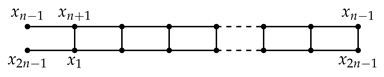
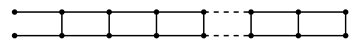
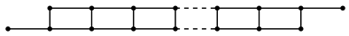
Theorem 6 implies that a cubic circulant graph is the disjoint union of one or more connected cubic circulant graphs. Furthermore, the only connected cubic circulant graphs are those circulant graphs that are isomorphic to either the circulant $C_{2n}(1,n)$ for any $n\ge 2$ or the circulant $C_{2n}(2,n)$ with $n>1$ odd (for the second circulant, if n is not odd, then Theorem 6 implies that this circulant is not connected). Recall from Theorem 1 $(i)$ that, to compute the regularity of a graph, it is enough to compute the regularity of each connected component. 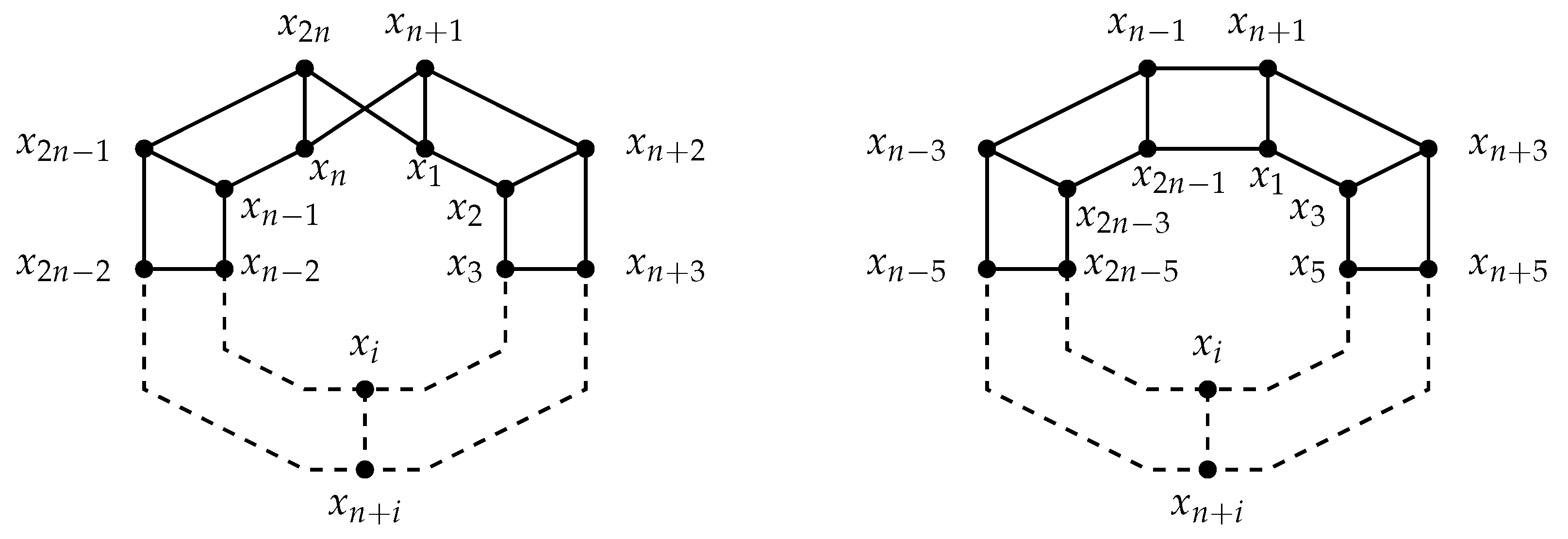Therefore, it suffices to compute the regularity of the edge ideals of $C_{2n}(1,n)$ and $C_{2n}(2,n)$ with n odd. Moving forward, unless stated otherwise, we will restrict to connected cubic circulant graphs. Note it will be convenient to use the representation and labelling of these two graphs as in Figure 2.

Our strategy is to use Theorem 4 to compute the regularity of these two graphs. Thus, we need bounds on $\mathrm{reg}(I(G))$ and $\mathrm{pd}(I(G))$ and information about the reduced Euler characteristic of $\mathrm{Ind}(G)$ when $G=C_{2n}(1,n)$ or $C_{2n}(2,n)$.

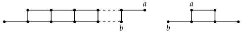
We first bound the regularity and the projective dimension. We introduce the following three families of graphs, where the $t\ge 1$ denotes the number of “squares”:

(i)

The family $A_t$:

(ii)

The family $B_t$:

(iii)

The family $D_t$:

Lemma 3. 

With the notation as above, we have:

(i)

If $G=A_t$, then:

$$\mathrm{reg}(I(G))\le \left\{\begin{array}{cc}\frac{t+4}{2}\hfill & if t even\hfill \\ \frac{t+3}{2}\hfill & if t odd\hfill \end{array}\right.and\mathrm{pd}(I(G))\le \left\{\begin{array}{cc}\frac{3t}{2}+1\hfill & if t even\hfill \\ \frac{3(t-1)}{2}+2\hfill & if t odd.\hfill \end{array}\right.$$

(ii)

If $G=B_t$, then

$$\mathrm{reg}(I(G))\le \left\{\begin{array}{cc}\frac{t+4}{2}\hfill & if t even\hfill \\ \frac{t+3}{2}\hfill & if t odd.\hfill \end{array}\right.$$

(iii)

If $G=D_t$ and $t=2l+1$ with l an odd number, then $\mathrm{reg}(I(G))\le \frac{t+3}{2}$.

Proof. 

$(i)$ The proof is by induction on t. Via a direct computation (for example, using Macaulay2 [19]), one finds $\mathrm{reg}(I(A_1))=2$, $\mathrm{reg}(I(A_2))=3$, $\mathrm{pd}(I(A_1))=2$, and $\mathrm{pd}(I(A_2))=4$. Our values agree with the upper bounds given in the statement, so the base cases hold.

Now, suppose that $t\ge 3$. The graph $A_t$ can be decomposed into the subgraphs $A_1$ and $A_{t-2}$, i.e.,

Suppose that t is even. By Theorem 2 and by induction (and the fact that $\mathrm{reg}(R/I)=\mathrm{reg}(I)-1)$, we get:

$$\mathrm{reg}(R/I(A_t))\le \mathrm{reg}(R/I(A_1))+\mathrm{reg}(R/I(A_{t-2}))\le 1+\frac{(t-2)+4}{2}-1=\frac{t+4}{2}-1$$

and:

$$\mathrm{pd}(I(A_t))\le \mathrm{pd}(I(A_1))+\mathrm{pd}(I(A_{t-2})+1\le 2+\frac{3(t-2)}{2}+1+1=\frac{3t}{2}+1.$$

Because the proof for when t is odd is similar, we omit it.

$(ii)$ A direct computation shows $\mathrm{reg}(I(B_1))=2$ and $\mathrm{reg}(I(B_2))=3$. If $t\ge 3$, we decompose $B_t$ into the subgraphs $B_1$ and $A_{t-2}$, i.e.,

Suppose that t is even. Since $\mathrm{reg}(I(B_1))=2$, Theorem 2 and Part (i) above give us:

$$\mathrm{reg}(R/I(B_t))\le \mathrm{reg}(R/I(B_1))+\mathrm{reg}(R/I(A_{t-2}))\le \frac{(t-2)+4}{2}=\frac{t+2}{2}.$$

Therefore, $\mathrm{reg}(I(B_t))\le \frac{t+2}{2}+1=\frac{t+4}{2}$. When t is odd, the proof is similar.

$(iii)$ Because $t=2l+1$ with l odd, the graph $D_t$ can be decomposed into $l+1$ subgraphs of the form $A_1$, i.e.,

Since $\mathrm{reg}(I(A_1))=2$, by Theorem 2, we get $\mathrm{reg}(R/I(D_t))\le (l+1)\mathrm{reg}(R/I(A_1))=l+1$. Thus, $\mathrm{reg}(I(D_t))\le l+2=\frac{t+3}{2}$. ☐

Remark 2. 

In the above proof, we relied on computer computations for our base case. In general, the graded Betti numbers of an ideal may depend on the characteristic of the ground field. However, as shown by Katzman [20], the Betti numbers of edge ideals of graphs on 11 or less vertices are independent of the characteristic. Since the graphs in our induction steps have 11 or less vertices, the values found for our base cases hold in all characteristics.

We now bound the projective dimensions of the edge ideals of $C_{2n}(1,n)$ and $C_{2n}(2,n)$. In the next two lemmas, we assume that $n\ge 4$. However, as we show in Theorem 8, the bounds (in fact, they are equalities) given in these lemmas also hold if $n=2$ or 3, i.e., if $G=C_4(1,2),C_6(1,3)$ or $C_6(2,3)$.

Lemma 4. 

Let $n\ge 4$.

(i)

If $G=C_{2n}(1,n)$, then:

$$\mathrm{pd}(I(G))\le \left\{\begin{array}{cc}3k-1\hfill & if n=2k\hfill \\ 3k+1\hfill & if n=2k+1.\hfill \end{array}\right.$$

(ii)

If $G=C_{2n}(2,n)$, then $\mathrm{pd}(I(G))\le 3k+1$ where $n=2k+1$.

Proof. 

$(i)$ Let $G=C_{2n}(1,n)$, and suppose that $n=2k+1$. The graph $C_{2n}(1,n)$ can be decomposed into the subgraphs $A_1$ and $A_{2k-2}$, i.e.,

Note that since $n\ge 4$ and n is odd, $2k-2\ge 2$. Combining Theorem 2 and Lemma 3, we get:

$$\mathrm{pd}(I(C_{2n}(1,n)))\le \mathrm{pd}(I(A_{2k-2}))+\mathrm{pd}(I(A_1))+1\le \left(\frac{3(2k-2)}{2}+1\right)+3=3k+1.$$

If $n=2k$, $C_{2n}(1,n)$ can be decomposed as in the previous case with the only difference being that $C_{2n}(1,n)$ can be decomposed into the union of the subgraphs $A_1$ and $A_{2k-3}$. By Theorem 2 and Lemma 3:

$$\mathrm{pd}(I(C_{2n}(1,n)))\le \mathrm{pd}(I(A_{2k-3}))+\mathrm{pd}(I(A_1))+1\le \left(\frac{3(2k-4)}{2}+2\right)+3=3k-1.$$

$(ii)$ Let $G=C_{2n}(2,n)$ with $n=2k+1$. We can draw G as:

The previous representation of G contains 2k squares. Then, the graph G can be decomposed into the subgraphs A₁ and $A_{2k-2}$, and the proof runs as in (i). ☐

We now determine bounds on the regularity.

Lemma 5. 

Let $n\ge 4$.

(i)

If $G=C_{2n}(1,n)$, then:

$$\mathrm{reg}(I(G))\le \left\{\begin{array}{cc}k+1\hfill & if n=2k, or if n=2k+1 and k odd\hfill \\ k+2\hfill & if n=2k+1 and k even.\hfill \end{array}\right.$$

(ii)

If $G=C_{2n}(2,n)$, then

$$\mathrm{reg}(I(G))\le \left\{\begin{array}{cc}k+1\hfill & if n=2k+1 and k even\hfill \\ k+2\hfill & if n=2k+1 and k odd.\hfill \end{array}\right.$$

Proof. 

$(i)$ Let $G=C_{2n}(1,n)$. We consider three cases.

Case 1. 

$n=2k$.

In Lemma 4 $(i)$, we saw that G can be decomposed into the subgraphs $A_1$ and $A_{2k-3}$. By Theorem 2 and Lemma 3, we get:

$$\mathrm{reg}(R/I(G))\le \mathrm{reg}(R/I(A_1))+\mathrm{reg}(R/I(A_{2k-3}))\le k.$$

Case 2. 

$n=2k+1$ with k an odd number.

Using Theorem 1 $(v)$, we have:

$$\mathrm{reg}(I(G))\in \{\mathrm{reg}(I(G\setminus x_1),\mathrm{reg}(I(G\setminus N_G\left[x_1\right])+1\}.$$

If we set $W=G\setminus x_1$, then by applying Theorem 1 $(v)$ again, we have:

$$\mathrm{reg}(I(G))\in \{\mathrm{reg}(I(W\setminus x_{n+1}),\mathrm{reg}(I(W\setminus N_W\left[x_{n+1}\right])+1,\mathrm{reg}(I(G\setminus N_G\left[x_1\right])+1\}.$$

We have $G\setminus N_G\left[x_1\right]\cong W\setminus N_W\left[x_{n+1}\right]\cong D_{2k-3}$. Moreover, $2k-3=2(k-2)+1$, and since k is an odd number, $k-2$ is also odd. Thus, by Lemma 3 $(iii)$, we obtain $\mathrm{reg}(I(D_{2k-3}))\le \frac{2k-3+3}{2}=k$. On the other hand, the graph $W\setminus x_{n+1}=(G\setminus x_1)\setminus x_{n+1}\cong B_{2k-1}$, so by Lemma 3 $(ii)$, we have $\mathrm{reg}(I(W\setminus x_{n+1}))\le \frac{2k-1+3}{2}\le k+1$. Thus, $\mathrm{reg}(I(G))\le k+1$.

Case 3. 

$n=2k+1$ with k an even number.

In Lemma 4 $(i)$, we saw that G can be decomposed into the subgraphs $A_1$ and $A_{2k-2}$, and the proof runs as in Case 1.

$(ii)$ Let $G=C_{2n}(2,n)$. We consider two cases.

Case 1. 

$n=2k+1$ with k an even number.

As in the second case of $(i)$, by Theorem 1 $(v)$, we have:

$$\mathrm{reg}(I(G))\in \{\mathrm{reg}(I(W\setminus x_{n+1}),\mathrm{reg}(I(W\setminus N_W\left[x_{n+1}\right])+1,\mathrm{reg}(I(G\setminus N_G\left[x_1\right])+1\}.$$

where $W=G\setminus x_1$. In particular, $W\setminus N_W\left[x_{n+1}\right]\cong G\setminus N_G\left[x_1\right]$. The graph $G\setminus N_G\left[x_1\right]$ can be represented as:

The previous representation of $G\setminus N_G\left[x_1\right]$ contains 2k − 3 squares. It follows that $G\setminus N_G\left[x_1\right]$ can be decomposed into the subgraphs $D_{2k-5}$ and A₁, i.e.,

Note that 2k − 5 = 2(k − 3) + 1, and because k is even, then k − 3 is odd. Using Theorem 2 and Lemma 3, we get:

$$\mathrm{reg}(R/I(G\setminus N_G\left[x_1\right]))\le \mathrm{reg}(R/I(D_{2k-5}))+\mathrm{reg}(R/I(A_1))\le \frac{2k-2}{2}=k-1.$$

The graph $W\setminus x_{n+1}\cong B_{2k-1}$. Therefore, by Lemma 3 $(ii)$, we have $\mathrm{reg}(I(W\setminus x_{n+1}))\le \frac{2k-1+3}{2}=k+1$. Consequently, $\mathrm{reg}(I(G))\le k+1$, as desired.

Case 2. 

$n=2k+1$ with k an odd number.

The result follows from the fact that the graphs $C_{2n}(2,n)$ can be decomposed into the subgraphs $A_1$ and $A_{2k-2}$ as seen in Lemma 4, and so, $\mathrm{reg}(I(G))\le \mathrm{reg}(I(A_1))+\mathrm{reg}(I(A_{2k-2}))-1$. ☐

Our final ingredient is a result of Hoshino ([21], Theorem 2.26) (also see Brown–Hoshino ([22]), Theorems 3.2 and 3.5), which describes the independence polynomial for cubic circulant graphs.

Theorem 7 

([21,22]). For each $n\ge 3$, set:

$$I_n(x)=1+\sum _{\ell =0}^{\lfloor \frac{n-2}{4}\rfloor }\frac{2n}{2\ell +1}\left(\genfrac{}{}{0pt}{}{n-2\ell -2}{2\ell }\right)x^{2\ell +1}{(1+x)}^{n-4\ell -2}.$$

(i)

If $G=C_{2n}(1,n)$ with n even, or if $G=C_{2n}(2,n)$ with n odd, then $I(G,x)=I_n(x)$.

(ii)

If $G=C_{2n}(1,n)$ and n is odd, then $I(G,x)=I_n(x)+2x^n$.

We now come to the main result of this section.

Theorem 8. 

Let $1\le a<n$ and $t=\gcd (2n,a)$.

(a)

If $\frac{2n}{t}$ is even, then:

$$\mathrm{reg}(I(C_{2n}(a,n)))=\left\{\begin{array}{cc}kt+1\hfill & if \frac{n}{t}=2k, or \frac{n}{t}=2k+1 with k an odd number\hfill \\ (k+1)t+1\hfill & if \frac{n}{t}=2k+1 with k an even number.\hfill \end{array}\right.$$

(b)

If $\frac{2n}{t}$ is odd, then:

$$\mathrm{reg}(I(C_{2n}(a,n)))=\left\{\begin{array}{cc}\frac{kt}{2}+1\hfill & if \frac{2n}{t}=2k+1 with k an even number\hfill \\ \frac{(k+1)t}{2}+1\hfill & if \frac{2n}{t}=2k+1 with k an odd number.\hfill \end{array}\right.$$

Proof. 

The formulas can be verified directly for the special cases that $n=2$ (i.e., $G=C_4(1,2)$) or $n=3$ (i.e., $G=C_6(1,3)$ and $C_6(2,3)$). We can therefore assume $n\ge 4$. In light of Theorem 6 and Theorem 1 $(i)$, it will suffice to prove that the inequalities of Lemma 5 are actually equalities. We will make use of Theorem 4. We consider five cases, where the proof of each case is similar.

Case 1. 

$G=C_{2n}(1,n)$ with $n=2k$.

In this case, Lemma 4 gives $\mathrm{pd}(I(G))\le 3k-1$, and Lemma 5 gives $\mathrm{reg}(I(G))\le k+1$. Furthermore, since $\tilde{\chi }(\mathrm{Ind}(G))=-I(G,-1)$ by Equation (2), Theorem 7 gives $\tilde{\chi }(\mathrm{Ind}(G))=-1$ if $n\ne 4m+2$, and $\tilde{\chi }(\mathrm{Ind}(G))=3$ if $n=4m+2$. Because G has $4k=(k+1)+(3k-1)$ vertices and since $\tilde{\chi }(\mathrm{Ind}(G))\ne 0$, Theorem 4 $(ii)$ implies $\mathrm{reg}(I(G))=k+1$.

Case 2. 

$G=C_{2n}(1,n)$ with $n=2k+1$ and k even.

We have $\mathrm{reg}(I(G))\le k+2$ and $\mathrm{pd}(I(G))\le 3k+1=(4k+2)-(k+2)+1=n-(k+2)+1$ by Lemmas 4 and 5, respectively. Because n is odd, $\tilde{\chi }(\mathrm{Ind}(G))=-[I_n(-1)+2{(-1)}^n]=-[1-2]=1>0$. Therefore, $\mathrm{reg}(I(G))=k+2$ by Theorem 4 $(i)$ $(a)$ because $k+2$ is even and $\tilde{\chi }(\mathrm{Ind}(G))=1>0$.

Case 3. 

$G=C_{2n}(1,n)$ with $n=2k+1$ and k odd.

We have $\mathrm{reg}(I(G))=k+1$ by Theorem 4 $(ii)$ because $\mathrm{reg}(I(G))\le k+1$ (Lemma 5), $\mathrm{pd}(I(G))\le 3k+1$ (Lemma 4), $2n=4k+2$ is the number of variables, and $\tilde{\chi }(\mathrm{Ind}(G))=-1\ne 0$.

Case 4. 

$G=C_{2n}(2,n)$ with $n=2k+1$ and k even.

We have $\mathrm{reg}(I(G))=k+1$ from Theorem 4 $(ii)$ since $\mathrm{reg}(I(G))\le k+1$ (Lemma 5), $\mathrm{pd}(I(G))\le 3k+1$ (Lemma 4), and $\tilde{\chi }(\mathrm{Ind}(G))=-I(G,-1)=-1\ne 0$ (Theorem 7).

Case 5. 

$G=C_{2n}(2,n)$ with $n=2k+1$ and k odd.

In our final case, $\mathrm{reg}(I(G))\le k+2$ by Lemma 5, $\mathrm{pd}(I(G))\le 3k+1$ by Lemma 4. Since n is odd, $\tilde{\chi }(\mathrm{Ind}(G))=-I(G,-1)=-1<0$ by Theorem 7. Since k is odd, $k+2$ is odd. Because $2n=4k+2$ is the number of variables, we have $\mathrm{reg}(I(G))=k+2$ by Theorem 4 $(i)$ $(b)$.

These five cases now complete the proof. ☐