A Seventh-Order Scheme for Computing the Generalized Drazin Inverse

Abstract

One of the most important generalized inverses is the Drazin inverse, which is defined for square matrices having an index. The objective of this work is to investigate and present a computational tool in the form of an iterative method for computing this task. This scheme reaches the seventh rate of convergence as long as a suitable initial matrix is chosen and by employing only five matrix products per cycle. After some analytical discussions, several tests are provided to show the efficiency of the presented formulation.

1. Introduction

Drazin, in the pioneering work in [1], proposed and generalized a different type of outer inverse in associative rings and semigroups that does not possess the reflexivity feature but commutes with the element. The significance of this type of inverse and its calculation was then discussed wholly in [2]. Accordingly, several authors attempted to propose procedures for the calculation of generalized inverses. See, e.g., [3,4,5].

It is recalled that the smallest non-negative integer k such that [6]

$$\mathrm{rank}\left(A^k\right)=\mathrm{rank}\left(A^{k+1}\right),$$

(1)

is named as the matrix A’s index and is shown by $\mathrm{ind}\left(A\right)$. Furthermore, assume that A is an $N\times N$ matrix with complex entries. The Drazin inverse of A, shown by $A^D$, is the unique matrix X reading the following identities [7]:

• $A^{k}XA=A^k$,
• $XAX=X$,
• $AX=XA$.

Throughout the paper, with $A^{*}$, $\mathcal{R}\left(A\right)$, $\mathcal{N}\left(A\right)$, and $\mathrm{rank}\left(A\right)$, we show the conjugate transpose, the range, the null space, and the rank of $A\in {\mathbb{C}}^{N\times N}$, respectively [8]. It is remarked that if $\mathrm{ind}\left(A\right)=1$, X is named as the g-inverse or group inverse of A. In addition, if A is nonsingular, then it is easily seen that

$$indA=0,\mathrm{and}{A}^D=A^{-1}.$$

(2)

For the square system $Ax=b$, the general solution can be represented using the concept of the Drazin inverse as follows [7]:

$$x=A^{D}b+(I-A{A}^D)z,$$

(3)

wherein $z\in \mathcal{R}\left(A^{k-1}\right)+\mathcal{N}\left(A\right)$.

Methods in the category of iteration schemes for computing generalized inverses like the Drazin inverse are quite sensitive to the choice of the initial approximation. In fact, the convergence of the Schulz-type method can only be observed if the initial value is chosen correctly [9,10]. This selection can be done under special care on some criteria, as already discussed, and given in the literature for different types of outer inverses. For some in-depth discussions about this, one may refer to [11].

Authors in [12] showed that iterative Schulz-type schemes can be used for finding the Drazin inverse of square matrices both possessing real or complex spectra. Actually, the authors investigated the initial matrix below:

$$X_0=\alpha A^l,l\ge \mathrm{ind}\left(A\right)=k,$$

(4)

wherein the parameter $\alpha$ should be selected such that the criterion $\parallel I-A{X}_0\parallel <1$ is read. Employing the starting value (4) yields an iterative scheme for computing the famous Drazin inverse with second-order convergence.

It is in fact necessary to apply an appropriate initial matrix when calculating the Drazin inverse. One way is as follows [12,13]:

$$X_0=\frac{2}{\mathrm{Tr}\left(A^{k+1}\right)}{A}^k,$$

(5)

wherein $\mathrm{Tr}(·)$ stands for the trace of an arbitrary square matrix. Another fruitful initial matrix which could lead in converging sequence of matrices for computing the generalized Drazin inverse can be written as

$$X_0=\frac{1}{{2\parallel A\parallel }_2^{k+1}}{A}^k.$$

(6)

The Schulz method of the quadratic convergence rate for doing this task can be defined by [14]

$$X_{n+1}=X_n(2I-A{X}_n),n=0,1,2,\cdots ,$$

(7)

where I is the identity matrix and requires only two matrix products to achieve this rate per cycle.

Authors in [15] re-studied Chebyshev’s method for calculating $A_{MN}^{†}$ using a suitable initial value as follows:

$$X_{n+1}=X_n(3I-A{X}_n(3I-A{X}_n)),n=0,1,2,\cdots ,$$

(8)

with a third-order of convergence having three matrix products per cycle. Another scheme, having a cubic rate of convergence and a greater number of matrix products, was given by the same authors as follows:

$$X_{n+1}=X_n\left[I+\frac{1}{2}(I-A{X}_n)(I+{(2I-A{X}_n)}^2)\right],n=0,1,2,\cdots .$$

(9)

A general procedure for having p-order methods with a p number of matrix–matrix products was given in [16] (Chapter 5). For instance, the authors presented the following fourth-order scheme:

$$X_{n+1}=X_n(I+B_n(I+B_n(I+B_n))),n=0,1,2,\cdots ,$$

(10)

in which $B_n=I-A{X}_n$.

The main goal and motivation for investigating novel or useful matrix schemes for computing the Drazin inverse is not only because of the applications of such solvers in different kinds of mathematical problems [17,18] but also to improve the computational efficiency index. In fact, the hyperpower structure as given for a sample case in (10) requires a p number of matrix–matrix products to achieve a p rate of convergence. This leads to more and more inefficient methods from this class of methods, particularly when the order increases.

As such, motivated by extending efficient methods of higher orders for calculating generalized inverses, here we focus on a seventh-order scheme and discuss how we can reach this higher rate by employing only five matrix by matrix products. This will reveal a higher efficiency index for the discussed scheme in computing the Drazin inverse. For more studies and investigations in this field and related issues of generalized matrix inverses, interested readers are guided to [19,20,21,22].

The organization of this paper is as follows. In Section 1, we quickly review the definition, literature, and the need for development of higher order schemes. Section 2 is devoted to extending and proposing an efficient iterative expression for the Drazin inverse. It is derived that the scheme requires only five matrix–matrix products to achieve this rate.

Theoretical discussions with some concrete proofs are provided in Section 3, while Section 4 is oriented on the application of this scheme for computing the Drazin inverses. Results will reveal the effectiveness of this scheme for calculating the Drazin inverse. Lastly, some concluding comments are given in Section 5.

2. Derivation of an Efficient Formulation

Here, the aim is to present a competitive formulation for a member of the hyperpower family of iterations, so as to not only gain a high rate of convergence but also improve the computational efficiency index. In fact, we must factorize the formulation so as to gain the same high convergence rate but a lower number of matrix products.

Toward this objective, let us take into account the following seventh-order method from the family of hyperpower iteration schemes [23]:

$$\begin{array}{ccc}\hfill X_{n+1}& =& X_n(I+B_n+B_n^2+B_n^3+B_n^4+B_n^5+B_n^6).\hfill \end{array}$$

(11)

It is necessary to emphasize that we are looking for a seventh-order scheme and not a higher-order one, since we wish to hit several targets at the same time. First, the derived scheme for the Drazin inverse must be efficient, viz., it must improve the computational efficiency index of the existing solvers, as will be shown at the end of this section. Second, very high-order schemes might occasionally become hard for coding purposes, and this limits their application, so we aim to have this order be high but not so high. Besides, higher-order schemes mean that fewer stopping criteria (the computation of matrix norms) should be calculated per cycle, which is useful in terms of the elapsed time.

Now, to improve the performance of (11), we factorize (11) in what follows:

$$X_{n+1}=X_n\left(I+B_n(I+B_n)(I-B_n+B_n^2)(I+B_n+B_n^2)\right).$$

(12)

However, the formulation (12) needs six matrix–matrix multiplications, which is still not that useful for improving the computational index of efficiency theoretically. As such, doing more factorization would yield the following scheme:

$$X_{n+1}=X_n\left(I+(B_n+B_n^2)(I-B_n+B_n^2)(I+B_n+B_n^2)\right).$$

(13)

The scheme (13) requires five matrix products per cycle to achieve the seventh order of convergence. Noting that one reason for the need to propose and have an efficient higher scheme in the category of matrix Schulz-type methods is also in the fact that Schulz-type schemes of lower orders are quite slow at the initial stage of iterates, and this could yield a greater computational burden for finding the Drazin inverse [24]. In fact, it sometimes takes several iterates for the scheme to arrive at its convergence phase, and due to imposing some stopping termination based on matrix norms, this might add some more elapsed time for the application of lower-order schemes.

It is recalled that the definition of index of efficiency is given by [25]:

$$EI={\rho }^{\frac{1}{\kappa }},$$

(14)

wherein $\rho$ and $\kappa$ are the convergence rate and the total cost per cycle, respectively.

Hence, the efficiency indexes of different methods are reported by

$$EI\left(7\right)=2^{\frac{1}{2}}\simeq 1.41421,EI\left(8\right)=3^{\frac{1}{3}}\simeq 1.44225,$$

(15)

$$EI\left(9\right)=4^{\frac{1}{4}}\simeq 1.41421,EI\left(12\right)=7^{\frac{1}{6}}\simeq 1.38309,EI\left(13\right)=7^{\frac{1}{5}}\simeq 1.47577.$$

(16)

This shows that we have achieved our motivation by improving the efficiency index for calculating the Drazin inverse via a competitive formulation.

3. Seventh Rate of Convergence

Let us now recall some of the well-known lemmas we need in the rest of this section.

Proposition 1 

([26]). Assume that $M\in {\mathbb{C}}^{n\times n}$ and $\epsilon >0$ are given. There is at least one matrix norm $\parallel ·\parallel$ such that

$$\rho \left(M\right)\le \parallel M\parallel \le \rho \left(M\right)+ϵ,$$

(17)

wherein $\rho \left(M\right)$ shows the collection of all of M’s eigenvalues (in the maximum of absolute value sense).

Proposition 2 

([26]). If $P_{L,M}$ shows the projector on a space L on space M, then

(i) 

$P_{L,M}Q=Q$ if and only if $\mathcal{R}\left(Q\right)\subseteq L$,

(ii) 

$Q{P}_{L,M}=Q$ if and only if $\mathcal{N}\left(Q\right)\supseteq M$.

The proof of the main theorem concerning the convergence as well as its rate of (13) for calculating the generalized Drazin inverse is now addressed as follows.

Theorem 1.

Consider that $A\in {\mathbb{C}}^{N\times N}$ is a square singular matrix. In addition, let the initial value $X_0$ be selected via (4) or (5). Thence, the matrices ${\left\{X_n\right\}}_{n=0}^{n=\infty }$ generated via (13) satisfy the following error estimate for calculating the Drazin inverse:

$$\parallel A^D-X_n\parallel \le \parallel A^D\parallel \parallel I-A{X}_0{\parallel }^{7^n}.$$

(18)

In addition, the convergence order is seven.

Proof. 

To prove that the sequence is converging, we first take into consideration that

$$\begin{array}{cc}\hfill R_{n+1}& =I-A{X}_{n+1}\hfill \\ & =I-A\left(X_n\left(I+(B_n+B_n^2)(I-B_n+B_n^2)(I+B_n+B_n^2)\right)\right)\hfill \\ & =I-A\left(X_n\left(I+B_n(I+B_n)(I-B_n+B_n^2)(I+B_n+B_n^2)\right)\right)\hfill \\ & =I-A\left(X_n\left(I+B_n+B_n^2+B_n^3+B_n^4+B_n^5+B_n^6\right)\right)\hfill \\ & ={(I-A{X}_n)}^7\hfill \\ & =R_n^7,\hfill \end{array}$$

(19)

wherein $R_n=I-A{X}_n$. Employing a matrix norm on (19), we obtain that

$$\parallel R_{n+1}\parallel \le \parallel R_n{\parallel }^7.$$

(20)

Since $X_0$ is selected as in (4) or (5), we have

$$\mathcal{R}\left(X_0\right)\subseteq \mathcal{R}\left(A^k\right).$$

(21)

This could now be stated as

$$\mathcal{R}\left(X_n\right)\subseteq \mathcal{R}\left(X_{n-1}\right).$$

(22)

Thus, we can conclude that

$$\mathcal{R}\left(X_n\right)\subseteq \mathcal{R}\left(A^k\right),n\ge 0.$$

(23)

In a similar way, by defining the scheme by the left-multiplying of $X_n$, we can state that

$$\mathcal{N}\left(X_n\right)\supseteq \mathcal{N}\left(A^k\right),n\ge 0.$$

(24)

Now, an application of the definition of the Drazin inverse yields

$$A{A}^D=A^{D}A=P_{\mathcal{R}\left(A^k\right),\mathcal{N}\left(A^k\right)}.$$

(25)

Proposition 2, along with (23), (24), and (25) could lead to

$$X_{n}A{A}^D=X_n=A^{D}A{X}_n,n\ge 0.$$

(26)

To complete the proof, we proceed in what follows. The error matrix ${\delta }_n=A^D-X_n$ satisfies

$$\begin{array}{cc}\hfill {\delta }_n& =A^D-X_n\hfill \\ & =A^D-A^{D}A{X}_n\hfill \\ & =A^D\left(I-A{X}_n\right)\hfill \\ & =A^D{R}_n.\hfill \end{array}$$

(27)

Using (20), we obtain the following inequality

$$\parallel {\delta }_n\parallel =\parallel A^D\parallel \parallel R_n\parallel \le \parallel A^D\parallel \parallel R_0{\parallel }^{7^n},$$

(28)

which is an affirmation of (18). Employing (28) and Proposition 2, one gets that

$$\begin{array}{cc}\hfill A{\delta }_{n+1}& =A{A}^D-A{X}_{n+1}\hfill \\ & =A{A}^D-I+I-A{X}_{n+1}\hfill \\ & =A{A}^D-I+R_{n+1}.\hfill \end{array}$$

(29)

Note that the idempotent matrix $A{A}^D$ is the projector on $\mathcal{R}\left(A^k\right)$ along $\mathcal{N}\left(A^k\right)$, where $\mathcal{R}\left(A^k\right)$ denotes the range of $A^k$, and $\mathcal{N}\left(A^k\right)$ is the null space of $A^k$. Considering (19) and applying several simplifications, one obtains

$$A{\delta }_{n+1}=A{A}^D-I+R_n^7.$$

(30)

Now, by taking into account the following feature,

$${(I-A{A}^D)}^t=(I-A{A}^D),t\ge 1,$$

(31)

we can get that

$$\begin{array}{cc}\hfill (I-A{A}^D)A{\delta }_n& =(I-A{A}^D)A(A^D-X_n)\hfill \\ & =X_n-A{A}^D{V}_n\hfill \\ & =0.\hfill \end{array}$$

(32)

We obtain, for each $t\ge 1$, that (here we use (32) in simplifications)

$$\begin{array}{cc}\hfill {\left(R_n\right)}^t+A{A}^D-I& ={(I-A{V}_n)}^t+A{A}^D-I\hfill \\ & ={(I-A{A}^D+A{A}^D-A{V}_n)}^t+A{A}^D-I\hfill \\ & ={\left((I-A{A}^D)+A{\delta }_n\right)}^t+A{A}^D-I\hfill \\ & =I-A{A}^D+{\left(A{\delta }_n\right)}^t+A{A}^D-I\hfill \\ & ={\left(A{\delta }_n\right)}^t.\hfill \end{array}$$

(33)

From (33) and (30), we have

$$A{\delta }_{n+1}={\left(A{\delta }_n\right)}^7.$$

(34)

Taking matrix norms from both sides yields

$$\parallel A{\delta }_{n+1}\parallel \le \parallel A{\delta }_n{\parallel }^7.$$

(35)

Considering (35) and the second criterion of (1), we obtain that

$$\begin{array}{cc}\hfill \parallel {\delta }_{n+1}\parallel & =\parallel X_{n+1}-A^D\parallel \hfill \\ & =\parallel A^{D}A{V}_{n+1}-A^{D}A{A}^D\parallel \hfill \\ & =\parallel A^D(A{V}_{n+1}-A{A}^D)\parallel \hfill \\ & \le \parallel A^D\parallel \parallel A{\delta }_{n+1}\parallel \hfill \\ & \le \parallel A^D\parallel \parallel {\delta }_n{\parallel }^7.\hfill \end{array}$$

(36)

The relations in (36) yield the point that $X_n\to A^D$ as $n\to +\infty$ with the seventh order of convergence. The proof is complete.  □

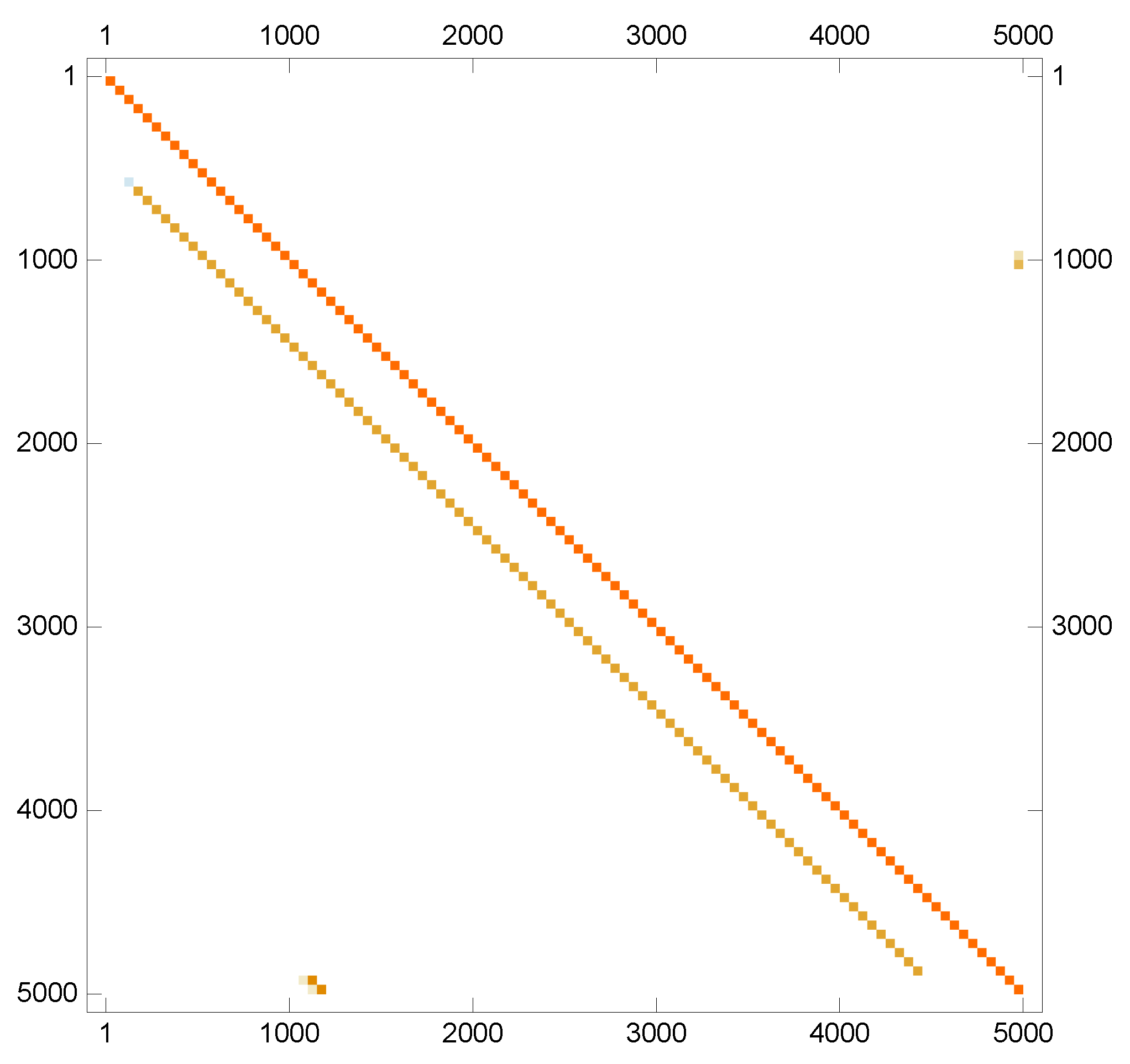
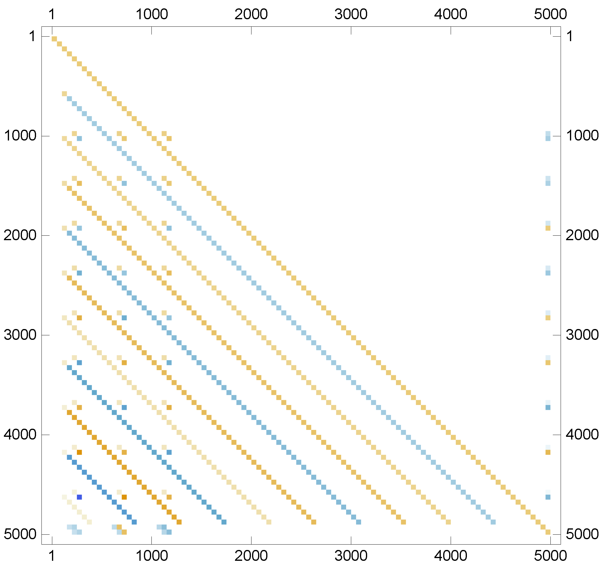
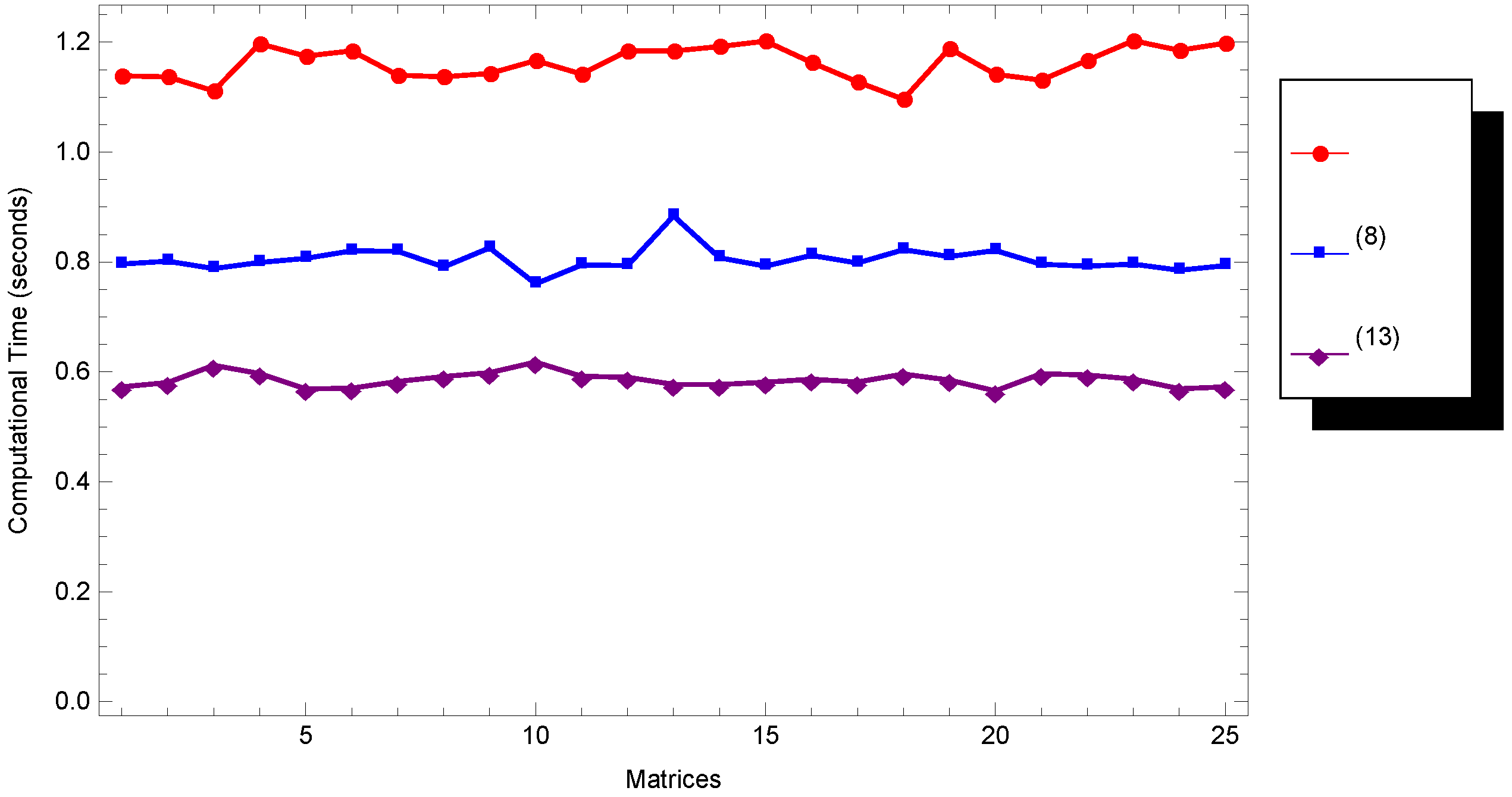
4. Computational Tests

The purpose of this section is to investigate the efficiency of our competitive formulation for computing the Drazin inverse, both theoretically and numerically. For such a task, we employ the challenging schemes (7), (8), and (13).

Here, we have simulated the tests in Mathematica 11.0, [27,28] and the time shown is in seconds. Noting that the compared methods are programmed in the same environment using the hardware CPU Intel Core i5 2430–M, 16 GB RAM in Windows 7 Ultimate with an SSD hard disk.

Test Problem 1.

The aim of this test is to testify the computation of the Drazin inverse for the following input [12]:

$$A=\left[\begin{array}{cccccccccccc}2& 0.4& 0& 0& 0& 0& 0& 0& 0& 0& 0& 0\\ -2& 0.4& 0& 0& 0& 0& 0& 0& 0& 0& 0& 0\\ -1& -1& 1& -1& 0& 0& 0& 0& -1& 0& 0& 0\\ -1& -1& -1& 1& 0& 0& 0& 0& 0& 0& 0& 0\\ 0& 0& 0& 0& 1& 1& -1& -1& 0& 0& -1& 0\\ 0& 0& 0& 0& 1& 1& -1& -1& 0& 0& 0& 0\\ 0& 0& 0& -1& -2& 0.4& 0& 0& 0& 0& 0& 0\\ 0& 0& 0& 0& 2& 0.4& 0& 0& 0& 0& 0& 0\\ 0& -1& 0& 0& 0& 0& 0& 0& 1& -1& -1& -1\\ 0& 0& 0& 0& 0& 0& 0& 0& -1& 1& -1& -1\\ 0& 0& 0& 0& 0& 0& 0& 0& 0& 0& 0.4& -2\\ 0& 0& 0& 0& 0& 0& 0& 0& 0& 0& 0.4& 2\end{array}\right],$$

at which $k=\mathrm{ind}\left(A\right)=3$. Here, the Drazin inverse is expressed by

$$A^D=\left[\begin{array}{cccccccccccc}0.25& -0.25& 0.& 0.& 0.& 0.& 0.& 0.& 0.& 0.& 0.& 0.\\ 1.25& 1.25& 0.& 0.& 0.& 0.& 0.& 0.& 0.& 0.& 0.& 0.\\ -1.66406& -0.992187& 0.25& -0.25& 0.& 0.& 0.& 0.& -0.0625& -0.0625& 0.& 0.15625\\ -1.19531& -0.679687& -0.25& 0.25& 0.& 0.& 0.& 0.& -0.0625& 0.1875& 0.6875& 1.34375\\ -2.76367& -1.04492& -1.875& -1.25& -1.25& 1.25& 1.25& 1.25& 1.48438& 2.57813& 3.32031& 6.64063\\ -2.76367& -1.04492& -1.875& -1.25& -1.25& 1.25& 1.25& 1.25& 1.48438& 2.57813& 4.57031& 8.51563\\ 14.1094& 6.30078& 6.625& 3.375& 5.& -3.& -5.& -5.& -4.1875& -8.5& -10.5078& -22.4609\\ -19.3242& -8.50781& -9.75& -5.25& -7.5& 4.5& 7.5& 7.5& 6.375& 12.5625& 15.9766& 33.7891\\ -0.625& -0.3125& 0.& 0.& 0.& 0.& 0.& 0.& 0.25& -0.25& -0.875& -1.625\\ -1.25& -0.9375& 0.& 0.& 0.& 0.& 0.& 0.& -0.25& 0.25& -0.875& -1.625\\ 0.& 0.& 0.& 0.& 0.& 0.& 0.& 0.& 0.& 0.& 1.25& 1.25\\ 0.& 0.& 0.& 0.& 0.& 0.& 0.& 0.& 0.& 0.& -0.25& 0.25\end{array}\right].$$

The results are obtained by applying the stop termination

$$\left|\right|X_{n+1}-X_n{\left|\right|}_1\le {10}^{-6},$$

(37)

and now by employing the definition in Section 1, we have for (13),

$$\begin{array}{l}\parallel A^{k+1}{X}_{n+1}-A^k{\parallel }_{\infty }\simeq 3.69638\times {10}^{-12},\\ \parallel X_{n+1}A{X}_{n+1}-X_{n+1}{\parallel }_{\infty }\simeq 8.43992\times {10}^{-10},\\ {\parallel A{X}_{n+1}-X_{n+1}A\parallel }_{\infty }\simeq 3.75205\times {10}^{-10}.\end{array}$$

(38)

It is also necessary to mention that the domain of validity for the proposed formulation (13) is not only limited to the Drazin inverse, and if a suitable initial approximation is used, under some assumptions we can construct a converging sequence of matrix iterates for other types of generalized inverses.

Test Problem 2.

In this test, we compare the results of various schemes for computing the regular inverse using the initial matrix

$$X_0=\frac{1}{{\parallel A\parallel }_F}{A}^{*},$$

(39)

the stopping condition (37), and the following complex matrices constructed in Mathematica:

N = 5000; no = 25;
ParallelTable[
  A[j] = SparseArray[
    {Band[{-100, 1100}] -> RandomReal[20], Band[{1, 1}] -> 2.,
     Band[{1000, -50}, {N - 20, N - 25}] -> {2.8, RandomReal[] + I},
     Band[{600, 150}, {N - 100, N - 400}] -> {-RandomReal[3], 3. + 3 I}
     },
    {N, N}, 0.],
  {j, no}
  ];
      

The plot of the large sparse matrices in Test Problem 2 is plotted in Figure 1, showing the sparsity pattern of these matrices, while the pattern of sparsity for the inverse matrix is provided in Figure 2. Figure 3 shows the clear superiority of the proposed formulation in computing the inverse of large sparse matrices.

Here, we give a simple Mathematica implementation of (13) in solving Test Problem 2:

For[j = 1, j <= number, j++,
  {
   X = A[j]/(Norm[A[j], "Frobenius"]^2);
   k = 1;
   X1 = 20 X;
   Time[j] = Part[
     While[k <= 75 && N[Norm[X - X1, 1]] >= 10^(-6),
        X1 = SparseArray[X];
        XX = Id - A[j].X1;
        X2 = XX.XX;
        X =
         Chop@
          SparseArray[
           X1.(Id + (XX + X2).(Id - XX + X2).(Id + XX + X2))];
        k++]; // AbsoluteTiming,
     1];
   }];
      

To apply our scheme in modern applications of numerical linear algebra getting involved with sparse large matrices, one may use some commands such as $\mathtt{SparseArray}\left[\right]$ for tackling matrices in sparse forms and subsequently reduce the computational effort and time for preserving the sparsity pattern and finding an approximate inverse. Such applications may occur in various types of problems like the ones in [29,30].

5. Conclusions

Following the motivation of proposing and extending efficient iteration schemes for computing generalized inverses, and particularly for Drazin inverses, in this work we have extended and discussed theoretically how we could achieve a seventh rate in a hyperpower structure for an iterative method. The scheme is a matrix product method and employs only five products to reach this rate. Clearly, the efficiency index will hit the bound $7^{1/5}\simeq 1.47577$.

Several computational tests for calculating the Drazin inverses of several randomly generated matrices were provided to show the superiority and stability of the scheme in doing this task. Other computational problems of different sizes for different matrices were also done and showed similar behavior and the superiority of (13) for the Drazin inverse.

References

1. Drazin, M.P. Pseudoinverses in associative rings and semigroups. Am. Math. Mon. 1958, 65, 506–514. [Google Scholar] [CrossRef]
2. Wilkinson, J.H. Note on the Practical Significance of the Drazin Inverse; Campbell, S.L., Ed.; Recent Applications of Generalized Inverses, Pitman Advanced Publishing Program, Research Notes in Mathematics, No. 66, Boston; NASA: Washington, DC, USA, 1982; pp. 82–99.
3. Kyrchei, I. Explicit formulas for determinantal representations of the Drazin inverse solutions of some matrix and differential matrix equations. Appl. Math. Comput. 2013, 219, 7632–7644. [Google Scholar] [CrossRef] [Green Version]
4. Liu, X.; Zhu, G.; Zhou, G.; Yu, Y. An analog of the adjugate matrix for the outer inverse A T , S ( 2 ) . Math. Prob. Eng. 2012, 2012, 591256. [Google Scholar]
5. Moghani, Z.N.; Khanehgir, M.; Karizaki, M.M. Explicit solution to the operator equation AD + FX*B = C over Hilbert C*-modules. J. Math. Anal. 2019, 10, 52–64. [Google Scholar]
6. Ben-Israel, A.; Greville, T.N.E. Generalized Inverses: Theory and Applications, 2nd ed.; Springer: New York, NY, USA, 2003. [Google Scholar]
7. Wei, Y. Index splitting for the Drazin inverse and the singular linear system. Appl. Math. Comput. 1998, 95, 115–124. [Google Scholar] [CrossRef]
8. Ma, H.; Li, N.; Stanimirović, P.S.; Katsikis, V.N. Perturbation theory for Moore–Penrose inverse of tensor via Einstein product. Comput. Appl. Math. 2019, 38, 111. [Google Scholar] [CrossRef]
9. Soleimani, F.; Soleymani, F.; Shateyi, S. Some iterative methods free from derivatives and their basins of attraction. Discret. Dyn. Nat. Soc. 2013, 2013, 301718. [Google Scholar] [CrossRef]
10. Soleymani, F. Efficient optimal eighth-order derivative-free methods for nonlinear equations. Jpn. J. Ind. Appl. Math. 2013, 30, 287–306. [Google Scholar] [CrossRef]
11. Pan, V.Y. Structured Matrices and Polynomials: Unified Superfast Algorithms; BirkhWauser: Boston, MA, USA; Springer: New York, NY, USA, 2001. [Google Scholar]
12. Li, X.; Wei, Y. Iterative methods for the Drazin inverse of a matrix with a complex spectrum. Appl. Math. Comput. 2004, 147, 855–862. [Google Scholar] [CrossRef]
13. Stanimirović, P.S.; Ciric, M.; Stojanović, I.; Gerontitis, D. Conditions for existence, representations, and computation of matrix generalized inverses. Complexity 2017, 2017, 6429725. [Google Scholar] [CrossRef]
14. Schulz, G. Iterative Berechnung der Reziproken matrix. Z. Angew. Math. Mech. 1933, 13, 57–59. [Google Scholar] [CrossRef]
15. Li, H.-B.; Huang, T.-Z.; Zhang, Y.; Liu, X.-P.; Gu, T.-X. Chebyshev-type methods and preconditioning techniques. Appl. Math. Comput. 2011, 218, 260–270. [Google Scholar] [CrossRef]
16. Krishnamurthy, E.V.; Sen, S.K. Numerical Algorithms: Computations in Science and Engineering; Affiliated East-West Press: New Delhi, India, 1986. [Google Scholar]
17. Ma, J.; Gao, F.; Li, Y. An efficient method to compute different types of generalized inverses based on linear transformation. Appl. Math. Comput. 2019, 349, 367–380. [Google Scholar] [CrossRef]
18. Soleymani, F.; Stanimirović, P.S.; Khaksar Haghani, F. On Hyperpower family of iterations for computing outer inverses possessing high efficiencies. Linear Algebra Appl. 2015, 484, 477–495. [Google Scholar] [CrossRef]
19. Qin, Y.; Liu, X.; Benítez, J. Some results on the symmetric representation of the generalized Drazin inverse in a Banach algebra. Symmetry 2019, 11, 105. [Google Scholar] [CrossRef]
20. Wang, G.; Wei, Y.; Qiao, S. Generalized Inverses: Theory and Computations; Science Press: Beijing, China; New York, NY, USA, 2004. [Google Scholar]
21. Xiong, Z.; Liu, Z. The forward order law for least Squareg-inverse of multiple matrix products. Mathematics 2019, 7, 277. [Google Scholar] [CrossRef]
22. Zhao, L. The expression of the Drazin Inverse with rank constraints. J. Appl. Math. 2012, 2012, 390592. [Google Scholar] [CrossRef]
23. Sen, S.K.; Prabhu, S.S. Optimal iterative schemes for computing Moore-Penrose matrix inverse. Int. J. Syst. Sci. 1976, 8, 748–753. [Google Scholar] [CrossRef]
24. Soleymani, F. An efficient and stable Newton–type iterative method for computing generalized inverse A T , S ( 2 ) . Numer. Algorithms 2015, 69, 569–578. [Google Scholar] [CrossRef]
25. Ostrowski, A.M. Sur quelques transformations de la serie de LiouvilleNewman. C.R. Acad. Sci. Paris 1938, 206, 1345–1347. [Google Scholar]
26. Jebreen, H.B.; Chalco-Cano, Y. An improved computationally efficient method for finding the Drazin inverse. Discret. Dyn. Nat. Soc. 2018, 2018, 6758302. [Google Scholar] [CrossRef]
27. Sánchez León, J.G. Mathematica Beyond Mathematics: The Wolfram Language in the Real World; Taylor & Francis Group: Boca Raton, FL, USA, 2017. [Google Scholar]
28. Wagon, S. Mathematica in Action, 3rd ed.; Springer: Berlin, Germany, 2010. [Google Scholar]
29. Soleymani, F. Efficient semi-discretization techniques for pricing European and American basket options. Comput. Econ. 2019, 53, 1487–1508. [Google Scholar] [CrossRef]
30. Soleymani, F.; Barfeie, M. Pricing options under stochastic volatility jump model: A stable adaptive scheme. Appl. Numer. Math. 2019, 145, 69–89. [Google Scholar] [CrossRef]
Figure 1. The sparsity pattern of matrices in Test Problem 2.
Mathematics 07 00622 g001
Figure 2. The sparsity pattern of the inverse matrix X = A 25 1 in Test Problem 2.
Mathematics 07 00622 g002
Figure 3. The CPU time required for different matrices in Test Problem 2.
Mathematics 07 00622 g003