A Mixed Finite Volume Element Method for Time-Fractional Reaction-Diffusion Equations on Triangular Grids

Abstract

In this article, the time-fractional reaction-diffusion equations are solved by using a mixed finite volume element (MFVE) method and the $L1$-formula of approximating the Caputo fractional derivative. The existence, uniqueness and unconditional stability analysis for the fully discrete MFVE scheme are given. A priori error estimates for the scalar unknown variable (in $L^2(\Omega )$-norm) and the vector-valued auxiliary variable (in ${\left(L^2(\Omega )\right)}^2$-norm and $\mathit{H}(\mathrm{div},\Omega )$-norm) are derived. Finally, two numerical examples in one-dimensional and two-dimensional spatial regions are given to examine the feasibility and effectiveness.

1. Introduction

Fractional partial differential equations (FPDEs) have received more and more attention from scholars in the fields of science and engineering because of their various practical applications [1,2,3,4,5,6]. Therefore, theoretical research and some problems of the solutions of FPDEs have been closely studied by many scholars [7,8,9,10,11]. However, there are still many FPDEs for which it is difficult to obtain analytic solutions. Thus, a lot of numerical techniques have been constructed and studied to solve FPDEs [12,13,14,15,16,17,18,19,20,21,22], including finite difference (FD) methods, finite element (FE) methods, mixed finite element (MFE) methods, spectral methods, (local) discontinuous Galerkin (L)DG methods and so on.

In recent years, finite volume (FV) and finite volume element (FVE) methods have been used to solve FPDEs by many scholars. Wang and Du [23] constructed a fast locally conservative FV method to solve steady-state space-fractional diffusion equations with Riesz fractional derivatives. Hejazi et al. [24,25] provided an FV method for the time-space two-sided fractional advection-dispersion equation and space fractional advection-dispersion equation, respectively. Zhuang et al. [26] proposed FV and FE methods for the space-fractional Boussinesq equation with Riemann-Liouville derivatives on a one-dimensional domain. Yang et al. [27] constructed an FV scheme with pretreatment Lanczos method to solve two-dimensional space fractional reaction-diffusion equations. Cheng et al. [28] provided an Eulerian-Lagrangian control volume method to solve the space-fractional advection-diffusion equations with Caputo fractional derivatives. Feng et al. [29] proposed an FV scheme to treat the two-sided space-fractional diffusion equation with Riemann-Liouville fractional derivatives. Jia and Wang [30,31] constructed fast FV schemes for two kinds of space-fractional differential equations, respectively. Simmons et al. [32] proposed an FV method to solve two-sided fractional diffusion equations with Riemann-Liouville derivatives. Jiang and Xu [33] constructed a monotone FV scheme to solve the time-fractional Fokker-Planck equation. Karaa et al. [34] proposed an FVE method to solve two-dimensional fractional subdiffusion problems with the Riemann-Liouville derivative. Karaa and Pani [35] applied an FVE method to solve the time-fractional diffusion equations with nonsmooth initial data.

In this article, we will develop a mixed finite volume element (MFVE) method to solve the time-fractional reaction-diffusion equations as follows

$$\begin{array}{c}\hfill \left\{\begin{array}{cc}{\displaystyle \frac{{\partial }^{\alpha }u(X,t)}{\partial t^{\alpha }}}-\epsilon \Delta u(X,t)+p\left(X\right)u(X,t)=f(X,t),\hfill & (X,t)\in \Omega \times J,\hfill \\ u(X,t)=0,\hfill & (X,t)\in \partial \Omega \times \overline{J},\hfill \\ u(X,0)=u_0\left(X\right),\hfill & X\in \overline{\Omega },\hfill \end{array}\right.\end{array}$$

(1)

where $\Omega \subset R^2$ is a bounded convex polygonal domain with boundary $\partial \Omega$, $J=(0,T]$ with $0<T<\infty$. The functions $u_0\left(X\right)$, $p\left(X\right)$ and $f(X,t)$ are smooth enough, the diffusion coefficient $\epsilon >0$. And there exist constants $p_0>0$ and $p_1>0$ such that $0<p_0\le p\left(X\right)\le p_1,\forall X\in \overline{\Omega }$. $\frac{{\partial }^{\alpha }u(X,t)}{\partial t^{\alpha }}$ is the Caputo fractional derivative defined by

$$\begin{array}{cc}\hfill {\displaystyle \frac{{\partial }^{\alpha }u(X,t)}{\partial t^{\alpha }}}={\displaystyle \frac{1}{\Gamma (1-\alpha )}}{\int }_0^t{\displaystyle \frac{\partial u(X,s)}{\partial s}}{\displaystyle \frac{\mathrm{d}s}{{(t-s)}^{\alpha }}},& 0<\alpha <1.\hfill \end{array}$$

(2)

Our aim is to construct an MFVE scheme [36,37,38,39,40,41] by combining the MFE method [42,43,44,45] with the FVE method [46,47,48,49,50,51] to treat the time Caputo fractional reaction-diffusion equation. The MFVE method can not only simultaneously compute several different quantities but also maintain the local conservativity, which is very important in computational fluid dynamics. In this article, we apply the $L1$-formula [52,53] to approximate the Caputo fractional derivative, introduce a vector-valued auxiliary variable to rewrite the model equation as the first-order coupled system, and approximate this coupled system by the MFVE method. We use the lowest order Raviart-Thomas ($R{T}_0$) space and the piecewise constant function space as the trial function spaces of the vector-valued auxiliary variable and scalar unknown variable, respectively. In terms of theoretical analysis, we give the existence, uniqueness and stability analysis, and obtain a priori error estimates for the scalar unknown variable (in $L^2(\Omega )$-norm) and the vector-valued auxiliary variable (in ${\left(L^2(\Omega )\right)}^2$-norm and $\mathit{H}(\mathrm{div},\Omega )$-norm). Further, we give two numerical examples in one-dimensional and two-dimensional spatial regions to verify the feasibility and effectiveness of the proposed scheme.

The remaining structure of the article is as follows. In Section 2, we present a fully discrete MFVE scheme for the time-fractional reaction-diffusion equation by introducing transfer operator ${\gamma }_h$ and the $L1$-formula of approximating the Caputo fractional derivative. In Section 3, the properties of transfer operator and truncation errors of $L1$-formula are given, and the generalized MFVE projection and its estimates are introduced. The existence, uniqueness, stability and convergence analysis for the MFVE scheme are analyzed in Section 4 and Section 5, respectively. Two numerical examples are given to verify the feasibility and effectiveness in Section 6. Throughout the article, we use the standard notations and definitions of the Sobolev spaces as in Reference [54]. The mark C will denote a generic positive constant which is independent of the spatial mesh parameter h and time discretization parameter $\tau$.

2. Fully Discrete MFVE Scheme

In order to formulate the MFVE approximate scheme, we introduce an auxiliary variable $\mathbf{\sigma }(X,t)=-\nabla u(X,t)$, and rewrite the problem (1) as

$$\left\{\begin{array}{cc}\left(a\right)\hfill & \mathbf{\sigma }(X,t)+\nabla u(X,t)=0,\hfill \\ \left(b\right)\hfill & {\displaystyle \frac{{\partial }^{\alpha }u(X,t)}{\partial t^{\alpha }}}+\epsilon \mathrm{div}\mathbf{\sigma }(X,t)+p\left(X\right)u(X,t)=f(X,t).\hfill \end{array}\right.$$

(3)

The associated mixed variational formulation of (3) is to find {u, $\mathbf{\sigma }$}: $[0,T]\to L^2(\Omega )\times \mathit{H}(\mathrm{div},\Omega )$ such that

$$\begin{array}{c}\hfill \left\{\begin{array}{ccc}\left(a\right)\hfill & (\mathbf{\sigma },\mathit{w})-(u,\mathrm{div}\mathit{w})=0,\hfill & \forall \mathit{w}\in \mathit{H}(\mathrm{div},\Omega ),\hfill \\ \left(b\right)\hfill & ({\displaystyle \frac{{\partial }^{\alpha }u}{\partial t^{\alpha }}},v)+\epsilon (\mathrm{div}\mathbf{\sigma },v)+(pu,v)=(f,v),\hfill & \forall v\in L^2(\Omega ),\hfill \\ \left(c\right)\hfill & u(X,0)=u_0\left(X\right),\mathbf{\sigma }(X,0)=-\nabla u_0\left(X\right),\hfill & \forall X\in \overline{\Omega },\hfill \end{array}\right.\end{array}$$

(4)

where $\mathit{H}(\mathrm{div},\Omega )=\{\mathit{w}\in {\left(L^2(\Omega )\right)}^2:\mathrm{div}\mathit{w}\in L^2(\Omega )\}$.

Now, we choose a quasi-uniform triangulation mesh ${\mathcal{T}}_h=\left\{K_B\right\}$ of the region $\Omega$, where $K_B$ represents a triangular element with B as the centre of gravity, referring to Figure 1. Let $h_{K_B}$ be the diameter of triangle $K_B$, and $h=max\left\{h_{K_B}\right\}$. The nodes are defined as the midpoint of the three sides of the triangle. $P_1,P_2,\cdots ,P_{M_0}$ represent the inner nodes and $P_{M_0+1},\cdots ,P_{M_S}$ represent the boundary nodes.

We select the $R{T}_0$ space ${\mathit{H}}_h$ as the trial function space for variable $\mathbf{\sigma }$, where

$$\begin{array}{c}\hfill {\mathit{H}}_h=\{{\mathit{w}}_h\in \mathit{H}(\mathrm{div},\Omega ):{\mathit{w}}_h{|}_K=(a+b{x}_1,c+b{x}_2),\forall K\in {\mathcal{T}}_h\},\end{array}$$

(5)

and select $L_h$ as the trial function space for variable u, where

$$\begin{array}{c}\hfill L_h=\{v_h\in L^2(\Omega ):v_h{|}_K\in P_0\left(K\right),\forall K\in {\mathcal{T}}_h\}.\end{array}$$

(6)

Next, we construct the dual partition ${\mathcal{T}}_h^{*}$, which is a union of quadrilaterals and triangles. For the interior node such as $P_3$, referring to Figure 1, the dual element $K_{P_3}^{*}$ is the quadrilateral $A_1{B}_1{A}_3{B}_2$, and contains triangles $K_L$ (with $\Delta A_1{B}_1{A}_3$) and $K_R$ (with $\Delta A_1{A}_3{B}_2$). For the boundary node such as $P_6$, the dual element $K_{P_6}^{*}$ is the triangle $K_I$ (with $\Delta A_4{A}_5{B}_3$).

Integrate (3) on the primal and dual partitions to obtain

$$\left\{\begin{array}{cc}\left(a\right)\hfill & {\int }_{K_P^{*}\cap K_j}(\mathbf{\sigma }+\nabla u)\mathrm{d}X=0,j=L,R,\mathrm{or}I,\hfill \\ \left(b\right)\hfill & {\int }_{K_B}({\displaystyle \frac{{\partial }^{\alpha }u}{\partial t^{\alpha }}}+\epsilon \mathrm{div}\mathbf{\sigma }+pu)\mathrm{d}X={\int }_{K_B}f\mathrm{d}X.\hfill \end{array}\right.$$

(7)

Similar to Reference [37], the transfer operator ${\gamma }_h:{\mathit{H}}_h\to {\left(L^2(\Omega )\right)}^2$ is defined by

$$\begin{array}{c}\hfill {\gamma }_h{\mathit{w}}_h=\sum _{j=1}^{M_0}\left({\mathit{w}}_h{{|}_{K_L}\left(P_j\right){\chi }_{K_j^{*}\cap K_L}+{\mathit{w}}_h|}_{K_R}\left(P_j\right){\chi }_{K_j^{*}\cap K_R}\right)+\sum _{j=M_0+1}^{M_S}{\mathit{w}}_h{|}_{K_I}\left(P_j\right){\chi }_{K_j^{*}},\end{array}$$

(8)

where ${\chi }_K$ represents the characteristic function of a set K. We select the range ${\mathbf{Y}}_h$ of the transfer operator ${\gamma }_h$ as the test function space. Then, we apply the transfer operator ${\gamma }_h$ and rewrite (7) to obtain the following form

$$\left\{\begin{array}{cc}\hfill \left(a\right)& (\mathbf{\sigma }+\nabla u,{\gamma }_h{\mathit{w}}_h)=0,\forall {\mathit{w}}_h\in {\mathit{H}}_h,\hfill \\ \hfill \left(b\right)& ({\displaystyle \frac{{\partial }^{\alpha }u}{\partial t^{\alpha }}}+\epsilon \mathrm{div}\mathbf{\sigma }+pu,v_h)=(f,v_h),\forall v_h\in L_h.\hfill \end{array}\right.$$

(9)

Making use of the Green theorem, we have

$$\begin{array}{cc}\hfill (\nabla u,{\gamma }_h{\mathit{w}}_h)& =\sum _{j=1}^{M_0}\left({\mathit{w}}_h{{|}_{K_L}(P_j){\int }_{\partial K_{P_j}^{*}\cap K_L}u\mathit{n}\mathrm{d}s+{\mathit{w}}_h|}_{K_R}(P_j){\int }_{\partial K_{P_j}^{*}\cap K_R}u\mathit{n}\mathrm{d}s\right)\hfill \\ & +\sum _{j=M_0+1}^{M_S}{\mathit{w}}_h{|}_{K_I}\left(P_j\right){\int }_{\partial K_{P_j}^{*}\setminus \partial \Omega }u\mathit{n}\mathrm{d}s\hfill \\ & \doteq b({\gamma }_h{\mathit{w}}_h,u),\forall {\mathit{w}}_h\in {\mathit{H}}_h,\hfill \end{array}$$

where $\mathit{n}$ represents the unit out-normal direction. We can easily obtain that $b({\gamma }_h{\mathit{w}}_h,v_h)=-(\mathrm{div}{\mathit{w}}_h,v_h)$, $\forall {\mathit{w}}_h\in {\mathit{H}}_h$, $\forall v_h\in L_h$. Then, we rewrite (9) to the following form

$$\left\{\begin{array}{cc}\hfill \left(a\right)& ({\mathbf{\sigma }}_h,{\gamma }_h{\mathit{w}}_h)-(\mathrm{div}{\mathit{w}}_h,u_h)=0,\forall {\mathit{w}}_h\in {\mathit{H}}_h,\hfill \\ \hfill \left(b\right)& ({\displaystyle \frac{{\partial }^{\alpha }{u}_h}{\partial t^{\alpha }}},v_h)+\epsilon (\mathrm{div}{\mathbf{\sigma }}_h,v_h)+(p{u}_h,v_h)=(f,v_h),\forall v_h\in L_h.\hfill \end{array}\right.$$

(10)

Now, let $0=t_0<t_1<\cdots <t_N=T$ be a equidistant grid of the time interval $[0,T]$ with step length $\tau =T/N$, for a positive integer N, and denote $t_n=n\tau ,n=0,1,\cdots ,N$. For a given function $\phi$ on $[0,T]$, we denote ${\phi }^n=\phi \left(t_n\right)$, ${\partial }_t{\phi }^n={\displaystyle \frac{{\phi }^n-{\phi }^{n-1}}{\tau }}.$ Following References [52,53], we can approximate the time-fractional derivative ${\displaystyle \frac{{\partial }^{\alpha }u(X,t)}{\partial t^{\alpha }}}$ at $t=t_n$ as follows

$$\begin{array}{cc}\hfill {\displaystyle \frac{{\partial }^{\alpha }u(X,t_n)}{\partial t^{\alpha }}}& ={\displaystyle \frac{1}{\Gamma (1-\alpha )}}{\int }_0^{t_n}{\displaystyle \frac{\partial u(X,s)}{\partial s}}{\displaystyle \frac{\mathrm{d}s}{{(t_n-s)}^{\alpha }}}\hfill \\ & ={\displaystyle \frac{{\tau }^{1-\alpha }}{\Gamma (2-\alpha )}}\sum _{k=0}^{n-1}{\widehat{b}}_k{\displaystyle \frac{u(X,t_{n-k})-u(X,t_{n-k-1})}{\tau }}+R_1^n\left(x\right)+R_2^n\left(x\right)\hfill \\ & ={\displaystyle \frac{{\tau }^{1-\alpha }}{\Gamma (2-\alpha )}}\sum _{k=0}^{n-1}{\widehat{b}}_k{\partial }_t{u}^{n-k}+R_t^n\left(x\right)\hfill \\ & ={\displaystyle \frac{{\tau }^{-\alpha }}{\Gamma (2-\alpha )}}\sum _{k=0}^n{b}_k^n{u}^k+R_t^n\left(x\right),\hfill \end{array}$$

(11)

where ${\widehat{b}}_k={(k+1)}^{1-\alpha }-k^{1-\alpha }$, $b_k^n={(n-k+1)}^{1-\alpha }-2{(n-k)}^{1-\alpha }+{(n-k-1)}^{1-\alpha }$, $b_n^n=1$, $b_0^n={(n-1)}^{1-\alpha }-n^{1-\alpha }$, $R_t^n\left(x\right)=R_1^n\left(x\right)+R_2^n\left(x\right)$, and

$$\begin{array}{c}{R}_1^n\left(x\right)={\displaystyle \frac{1}{\Gamma (1-\alpha )}}\sum _{k=1}^n{\int }_{t_{k-1}}^{t_k}{\displaystyle \frac{\partial u(X,s)}{\partial s}}{\displaystyle \frac{\mathrm{d}s}{{(t_n-s)}^{\alpha }}}-{\displaystyle \frac{{\tau }^{1-\alpha }}{\Gamma (1-\alpha )}}\sum _{k=0}^{n-1}{\widehat{b}}_k{\displaystyle \frac{\partial }{\partial t}}u(X,t_{n-k-1/2}),\hfill \\ R_2^n\left(x\right)={\displaystyle \frac{{\tau }^{1-\alpha }}{\Gamma (2-\alpha )}}\sum _{k=0}^{n-1}{\widehat{b}}_k({\displaystyle \frac{\partial }{\partial t}}u(X,t_{n-k-1/2})-{\partial }_t{u}^{n-k}).\hfill \end{array}$$

(12)

Denote $D_t^{\alpha }{\phi }^n={\displaystyle \frac{{\tau }^{-\alpha }}{\Gamma (2-\alpha )}}{\sum }_{k=0}^n{b}_k^n{\phi }^k$, then we have ${\displaystyle \frac{{\partial }^{\alpha }u(X,t_n)}{\partial t^{\alpha }}}=D_t^{\alpha }{u}^n+R_t^n\left(x\right)$.

Let $U^n$ and ${\mathit{Z}}^n$ be the approximate solutions of u and $\mathbf{\sigma }$ at $t=t_n$, respectively. Then we get the fully-discrete MFVE scheme to find $\{U^n,{\mathit{Z}}^n\}\in L_h\times {\mathit{H}}_h$, $n=1,2,\cdots ,N$, such that

$$\left\{\begin{array}{cc}\hfill \left(a\right)& ({\mathit{Z}}^n,{{\gamma }_h\mathbf{w}}_h)-(U^n,\mathrm{div}{\mathit{w}}_h)=0,\forall {\mathit{w}}_h\in {\mathit{H}}_h,\hfill \\ \hfill \left(b\right)& (D_t^{\alpha }{U}^n,v_h)+\epsilon (\mathrm{div}{\mathbf{Z}}^n,v_h)+(p\left(X\right)U^n,v_h)=(f^n,v_h),\forall v_h\in L_h,\hfill \end{array}\right.$$

(13)

where $\{U^0,{\mathit{Z}}^0\}\in L_h\times {\mathit{H}}_h$ satisfies

$$\left\{\begin{array}{cc}\hfill \left(a\right)& (U^0,v_h)=(u_0,v_h),\forall v_h\in L_h,\hfill \\ \hfill \left(b\right)& (Z^0,{\gamma }_h{\mathit{w}}_h)-(U^0,\mathrm{div}{\mathit{w}}_h)=0,\forall {\mathit{w}}_h\in {\mathit{H}}_h.\hfill \end{array}\right.$$

(14)

Remark 1.

(1) In practical numerical calculations, we need to apply the definition of $D_t^{\alpha }{\phi }^n$ to rewrite (13)$\left(b\right)$ into the following or other equations

$$\begin{array}{c}\hfill \frac{1}{\Gamma (2-\alpha )}(U^n,v_h)+\epsilon {\tau }^{\alpha }(\mathrm{div}{\mathit{Z}}^n,v_h)+{\tau }^{\alpha }(p\left(X\right)U^n,v_h)={\tau }^{\alpha }(f^n,v_h)-\frac{1}{\Gamma (2-\alpha )}\sum _{k=0}^{n-1}{b}_k^n(U^k,v_h),\forall v_h\in L_h.\end{array}$$

The above equation is also used when the existence and uniqueness of discrete solutions are proved in Section 4.

(2) Compared with the standard FE methods [17,18,19,20] and FVE methods [34,35], the MFVE methods can simultaneously compute the different physical quantities about the scalar unknown variable u (such as displacement) and the vector-valued auxiliary variable σ (such as flux).

(3) In this article, we consider the Caputo fractional reaction-diffusion equations. Actually, we can apply the conversion relationship between the Caputo derivative and the Riemann-Liouville derivative to approximate the Riemann-Liouville derivative.

3. Some Lemmas and Notations

From (11) and (12), we can know that the truncation errors $R_1^n\left(x\right)$, $R_2^n\left(x\right)$ and $R_t^n\left(x\right)$ will be estimated by the following lemma.

Lemma 1

([52] (Inequalities (3.2) and (3.3))). The truncation errors $R_1^n\left(x\right)$, $R_2^n\left(x\right)$ and $R_t^n\left(x\right)$ defined by (12) are bounded by

$$\begin{array}{c}\parallel R_1^n\left(x\right)\parallel \le C{\tau }^{2-\alpha },\parallel R_2^n\left(x\right)\parallel \le C{\tau }^2,\hfill \\ \parallel R_t^n\left(x\right)\parallel \le C({\tau }^2+{\tau }^{2-\alpha }),\hfill \end{array}$$

where $C>0$ is a generic constant which is independent of space-time grid step h and τ.

Lemma 2

([52] (See the proof of Theorem 3.2)). Let ${\phi }^k\ge 0,k=0,1,\cdots ,N$, which satisfy

$$\begin{array}{c}\hfill {\phi }^n\le -\sum _{k=1}^{n-1}{b}_k^n{\phi }^k+\zeta ,\end{array}$$

with $\zeta >0$, then there exists a constant $C>0$ independent of space-time grid step h and τ such that

$$\begin{array}{c}\hfill {\phi }^n\le C{\tau }^{-\alpha }\zeta ,n=1,2,\cdots ,N.\end{array}$$

Next, we give the properties of the transfer operator ${\gamma }_h$. For $\forall {\mathbf{w}}_h=(w_h^1,w_h^2)\in {\mathit{H}}_h$, the discrete seminorm and the norm are defined as follows

$$\begin{array}{c}\hfill |{\mathbf{w}}_h{|}_{1,h}^2=\sum _{K\in {\mathfrak{T}}_h}(\parallel \nabla w_h^1{\parallel }_{0,K}^2+\parallel \nabla w_h^1{\parallel }_{0,K}^2),\parallel {\mathbf{w}}_h{\parallel }_{1,h}^2=\parallel {\mathbf{w}}_h{\parallel }^2+{\left|{\mathbf{w}}_h\right|}_{1,h}^2.\end{array}$$

Lemma 3

([37] (Lemma 2.4)). The transfer operator ${\gamma }_h$ is bounded

$$\begin{array}{c}\hfill \parallel {\gamma }_h{\mathit{w}}_h\parallel \le \parallel {\mathit{w}}_h\parallel ,\forall {\mathit{w}}_h\in {\mathbf{H}}_h.\end{array}$$

Moreover, there exists a constant $C>0$ independent of h such that

$$\begin{array}{c}\parallel (I-{\gamma }_h){\mathit{w}}_h\parallel \le Ch\parallel {\mathit{w}}_h{\parallel }_{1,h},\forall {\mathit{w}}_h\in {\mathbf{H}}_h,\hfill \\ |({\mathit{w}}_h,(I-{\gamma }_h)z_h)|\le Ch\parallel {\mathit{w}}_h{\parallel }_{1,h}\parallel z_h\parallel ,\forall {\mathit{w}}_h,z_h\in {\mathbf{H}}_h,\hfill \\ |(\mathit{w},(I-{\gamma }_h)z_h){|\le Ch\parallel \mathit{w}\parallel }_1\parallel z_h\parallel ,\forall \mathit{w}\in {\left(H^1(\Omega )\right)}^2,\forall z_h\in {\mathbf{H}}_h.\hfill \end{array}$$

Lemma 4

([39] (Lemmas 3.3 and 3.4)). The following symmetry relation holds

$$\begin{array}{c}\hfill ({\gamma }_h{\mathit{w}}_h,z_h)=({\mathit{w}}_h,{\gamma }_h{z}_h),\forall {\mathit{w}}_h,z_h\in {\mathit{H}}_h,\end{array}$$

and there exists a constant ${\mu }_0>0$ independent of h such that

$$\begin{array}{c}\hfill ({\gamma }_h{\mathit{w}}_h,{\mathit{w}}_h)\ge {\mu }_0{\parallel {\mathit{w}}_h\parallel }^2,\forall {\mathit{w}}_h\in {\mathbf{H}}_h.\end{array}$$

Lemma 5.

Let ${\left\{{\mathbf{\psi }}^n\right\}}_{n=0}^{\infty }$ be a function sequence on $L^2(\Omega )$, then we have

$$\begin{array}{c}\hfill \left({\gamma }_h{\mathbf{\psi }}^n,\sum _{k=0}^n{b}_k^n{\mathbf{\psi }}^n\right)=\frac{1}{2}\left[({\mathbf{\psi }}^n,{\gamma }_h{\mathbf{\psi }}^n)+\sum _{k=0}^{n-1}{b}_k^n({\mathbf{\psi }}^k,{\gamma }_h{\mathbf{\psi }}^k)-\sum _{k=0}^{n-1}{b}_k^n({\mathbf{\psi }}^n-{\mathbf{\psi }}^k,{\gamma }_h({\mathbf{\psi }}^n-{\mathbf{\psi }}^k))\right].\end{array}$$

Proof. 

Noting that $-{\sum }_{k=0}^{n-1}{b}_k^n=1$, and applying Lemma 4, we obtain

$$\begin{array}{cc}\hfill \left({\gamma }_h{\mathbf{\psi }}^n,\sum _{k=0}^n{b}_k^n{\mathbf{\psi }}^n\right)& =({\gamma }_h{\mathbf{\psi }}^n,b_n^n{\mathbf{\psi }}^n)+\left({\gamma }_h{\mathbf{\psi }}^n,\sum _{k=0}^{n-1}{b}_k^n{\mathbf{\psi }}^n\right)\hfill \\ & =\frac{1}{2}({\gamma }_h{\mathbf{\psi }}^n,{\mathbf{\psi }}^n)+\frac{1}{2}\sum _{k=0}^{n-1}{b}_k^n\left[-({\gamma }_h{\mathbf{\psi }}^n,{\mathbf{\psi }}^n)+({\gamma }_h{\mathbf{\psi }}^n,{\mathbf{\psi }}^k)+({\gamma }_h{\mathbf{\psi }}^k,{\mathbf{\psi }}^n)\right].\hfill \end{array}$$

(15)

Applying Lemma 4, we can have the following equation

$$\begin{array}{c}\hfill -({\gamma }_h{\mathbf{\psi }}^n,{\mathbf{\psi }}^n)+({\gamma }_h{\mathbf{\psi }}^n,{\mathbf{\psi }}^k)+({\gamma }_h{\mathbf{\psi }}^k,{\mathbf{\psi }}^n)=({\gamma }_h{\mathbf{\psi }}^k,{\mathbf{\psi }}^k)-({\gamma }_h({\mathbf{\psi }}^k-{\mathbf{\psi }}^n),({\mathbf{\psi }}^k-{\mathbf{\psi }}^n)).\end{array}$$

(16)

Substituting the above equation into (15), we obtain the desired result. □

Now, we introduce the generalized MFVE projection $({\tilde{u}}_h,{\tilde{\mathbf{\sigma }}}_h):$ $[0,T]\to L_h\times {\mathit{H}}_{\mathit{H}}$, satisfies

$$\left\{\begin{array}{cc}\hfill \left(a\right)& (\mathbf{\sigma }-{\tilde{\mathbf{\sigma }}}_h,{{\gamma }_h\mathit{w}}_h)-(u-{\tilde{u}}_h,\mathrm{div}{\mathit{w}}_h)=-(\mathbf{\sigma },(I-{\gamma }_h){\mathit{w}}_h),\forall {\mathit{w}}_h\in {\mathit{H}}_h,\hfill \\ \hfill \left(b\right)& (\mathrm{div}(\mathbf{\sigma }-{\tilde{\mathbf{\sigma }}}_h),v_h)=0,\forall v_h\in L_h.\hfill \end{array}\right.$$

(17)

According to Reference [40], the above generalized MFVE projection satisfies the following estimates.

Lemma 6

([40] (Theorems 3.1 and 3.2)). Suppose $({\tilde{u}}_h,{\tilde{\mathbf{\sigma }}}_h)$ satisfies (17), then there exists a constant $C>0$ independent of h and t such that, for $i=0,1$

$$\begin{array}{c}\parallel \frac{{\partial }^i\mathbf{\sigma }}{\partial t^i}-\frac{{\partial }^i{\tilde{\mathbf{\sigma }}}_h}{\partial t^i}\parallel \le Ch\parallel \frac{{\partial }^i\mathbf{\sigma }}{\partial t^i}{\parallel }_1,\frac{{\partial }^i\mathbf{\sigma }}{\partial t^i}\in {\left(H^1(\Omega )\right)}^2,\hfill \end{array}$$

(18)

$$\begin{array}{c}\parallel \mathrm{div}\frac{{\partial }^i\mathbf{\sigma }}{\partial t^i}-\mathrm{div}\frac{{\partial }^i{\tilde{\mathbf{\sigma }}}_h}{\partial t^i}\parallel \le Ch\parallel \frac{{\partial }^i\mathbf{\sigma }}{\partial t^i}{\parallel }_1,\frac{{\partial }^i\mathbf{\sigma }}{\partial t^i}\in {\mathbf{H}}^1(\mathrm{div},\Omega ),\hfill \end{array}$$

(19)

$$\begin{array}{c}\parallel \frac{{\partial }^{i}u}{\partial t^i}-\frac{{\partial }^i\tilde{u}}{\partial t^i}\parallel \le Ch(\parallel \frac{{\partial }^i\sigma }{\partial t^i}{\parallel }_1+\parallel \frac{{\partial }^{i}u}{\partial t^i}{\parallel }_1),\frac{{\partial }^i\mathbf{\sigma }}{\partial t^i}\in {\left(H^1(\Omega )\right)}^2,\frac{{\partial }^{i}u}{\partial t^i}\in H^1(\Omega ),\hfill \end{array}$$

(20)

where ${\mathbf{H}}^1(\mathrm{div},\Omega )=\{\mathit{w}\in {\left(L^2(\Omega )\right)}^2:\mathrm{div}\mathit{w}\in H^1(\Omega )\}$.

4. Existence, Uniqueness and Stability Analysis for the MFVE Scheme

We first give the detailed proof of the existence and uniqueness for the MFVE scheme (13).

Theorem 1.

There exists a unique solution for the MFVE scheme (13).

Proof. 

Let ${\left\{{\mathbf{\varphi }}_i\right\}}_{i=1}^{M_S}$ and ${\left\{{\psi }_j\right\}}_{j=1}^{M_B}$ be the basis functions of the space ${\mathit{H}}_h$ and $L_h$, then ${\mathit{Z}}^n\in {\mathit{H}}_h$ and $U^n\in L_h$ are expressed as follows

$$\begin{array}{c}\hfill {\mathit{Z}}^n=\sum _{i=1}^{M_S}{z}_i^n{\mathbf{\varphi }}_i\left(x\right),U^n=\sum _{j=1}^{M_B}{u}_j^n{\psi }_j\left(x\right).\end{array}$$

Substituting the above expressions into (13), and taking ${\mathbf{w}}_h={\mathbf{\varphi }}_i(i=1,2,\cdots ,M_S)$ and $v_h={\psi }_j(j=1,2,\cdots ,M_B)$, then (13) can be expressed as a matrix form: find $\{{\mathbf{z}}^n,{\mathbf{u}}^n\}$ such that

$$\left[\begin{array}{cc}{A}_1& -C\\ \epsilon {\tau }^{\alpha }{C}^T& \frac{1}{\Gamma (2-\alpha )}{A}_2+{\tau }^{\alpha }{A}_3\end{array}\right]\left[\begin{array}{c}{\mathbf{z}}^n\\ {\mathbf{u}}^n\end{array}\right]=\left[\begin{array}{c}0\\ {\tau }^{\alpha }{F}^n-\frac{1}{\Gamma (2-\alpha )}\sum _{k=0}^{n-1}{b}_k^n{A}_2{\mathbf{u}}^k\end{array}\right],$$

(21)

where

$$\begin{array}{cc}{\mathbf{z}}^n={(z_1^n,z_2^n,\cdots ,z_{M_S}^n)}^T,\hfill & {\mathbf{u}}^n={(u_1^n,u_2^n,\cdots ,u_{M_B}^n)}^T,\hfill \\ A_1={\left(({\mathbf{\varphi }}_i,{\gamma }_h{\mathbf{\varphi }}_j)\right)}_{i,j=1,\cdots ,M_S},\hfill & A_2={\left(({\psi }_i,{\psi }_j)\right)}_{i,j=1,\cdots ,M_B},\hfill \\ A_3={\left((p{\psi }_i,{\psi }_j)\right)}_{i,j=1,\cdots ,M_B},\hfill & C={\left(({\psi }_i,\mathrm{div}{\mathbf{\varphi }}_j)\right)}_{i=1,\cdots ,M_B,j=1,\cdots ,M_S},\hfill \\ F^n={\left((f^n,{\psi }_j)\right)}_{j=1,\cdots ,M_B}^T.\hfill \end{array}$$

It should be noted that $A_1$, $A_2$ and $A_3$ are symmetric positive definite matrices. Noting that

$$\left[\begin{array}{cc}E& 0\\ -\epsilon {\tau }^{\alpha }{C}^T{A}_1^{-1}& E\end{array}\right]\left[\begin{array}{cc}{A}_1& -C\\ \epsilon {\tau }^{\alpha }{C}^T& \frac{1}{\Gamma (2-\alpha )}{A}_2+{\tau }^{\alpha }{A}_3\end{array}\right]=\left[\begin{array}{cc}{A}_1& -C\\ 0& G\end{array}\right],$$

(22)

where E is the identity matrix, $G=\frac{1}{\Gamma (2-\alpha )}{A}_2+{\tau }^{\alpha }{A}_3+\epsilon {\tau }^{\alpha }{C}^T{A}_1^{-1}C$, we have that G is a symmetric positive definite matrix and the coefficient matrix of linear equations (21) is invertible. Thus, linear Equations (21) have a unique solution, that is to say the MFVE scheme (13) has a unique solution. The proof of Theorem 1 has been completed. □

Next, we consider the stability for the MFVE scheme (13).

Theorem 2.

Let $\{U^n,{\mathit{Z}}^n\}$ be the solution of the MFVE scheme (13), then there exists a constant $C>0$ independent of h and τ such that

$$\begin{array}{c}\hfill \parallel U^n\parallel \le C\Gamma (2-\alpha )\underset{[0,T]}{sup}\parallel f\left(t\right)\parallel ,\parallel Z^n\parallel \le C\sqrt{\Gamma (2-\alpha )}\underset{[0,T]}{sup}\parallel f\left(t\right)\parallel .\end{array}$$

Proof. 

Choosing $v_h=U^n$ and ${\mathit{w}}_h={\mathit{Z}}^n$ in (13), we can obtain

$$\begin{array}{c}\hfill (D_t^{\alpha }{U}^n,U^n)+\epsilon ({\mathit{Z}}^n,{{\gamma }_h\mathit{Z}}^n)+(p\left(X\right)U^n,U^n)=(f^n,U^n).\end{array}$$

(23)

By virtue of the definition of $D_t^{\alpha }{U}^n$, we derive

$$\begin{array}{c}\hfill (D_t^{\alpha }{U}^n,U^n)=\frac{{\tau }^{-\alpha }}{\Gamma (2-\alpha )}{\parallel U^n\parallel }^2+\frac{{\tau }^{-\alpha }}{\Gamma (2-\alpha )}\sum _{k=0}^{n-1}{b}_k^n(U^k,U^n).\end{array}$$

(24)

Substituting (24) into (23), and applying Lemma 4, we have

$$\begin{array}{c}\hfill \parallel U^n{\parallel }^2\le -\sum _{k=0}^{n-1}{b}_k^n(U^k,U^n)+{\tau }^{\alpha }\Gamma (2-\alpha )(f^n,U^n).\end{array}$$

(25)

$$\begin{array}{c}\hfill \parallel U^n{\parallel }^2\le -\sum _{k=0}^{n-1}{b}_k^n\parallel U^k\parallel \parallel U^n\parallel +{\tau }^{\alpha }\Gamma (2-\alpha )\parallel f^n\parallel \parallel U^n\parallel ,\end{array}$$

The above inequality leads to the following result

$$\begin{array}{c}\hfill \parallel U^n\parallel \le -\sum _{k=0}^{n-1}{b}_k^n\parallel U^k\parallel +{\tau }^{\alpha }\Gamma (2-\alpha )\parallel f^n\parallel .\end{array}$$

(26)

Applying Lemma 2, we obtain

$$\begin{array}{c}\hfill \parallel U^n\parallel \le C\Gamma (2-\alpha )\underset{[0,T]}{sup}\parallel f\left(t\right)\parallel .\end{array}$$

(27)

Now, making use of (13)(a) and (14)(b), we have

$$\begin{array}{c}\hfill (D_t^{\alpha }{\mathit{Z}}^n,{{\gamma }_h\mathit{w}}_h)-(D_t^{\alpha }{U}^n,\mathrm{div}{\mathit{w}}_h)=0,\forall {\mathit{w}}_h\in {\mathit{H}}_h.\end{array}$$

(28)

Choosing ${\mathit{w}}_h={\mathit{Z}}^n$ in (28) and $v_h=D_t^{\alpha }{U}^n$ in (13)(b), we have

$$\begin{array}{c}\hfill \parallel D_t^{\alpha }{U}^n{\parallel }^2+\epsilon (D_t^{\alpha }{\mathit{Z}}^n,{{\gamma }_h\mathit{Z}}^n)+(p\left(X\right)U^n,D_t^{\alpha }{U}^n)=(f^n,D_t^{\alpha }{U}^n).\end{array}$$

(29)

Apply Lemma 5 in (29) and note that

$$\begin{array}{c}\hfill -\sum _{k=0}^{n-1}{b}_k^n\left({\mathit{Z}}^n-{\mathit{Z}}^k,{\gamma }_h({\mathit{Z}}^n-{\mathit{Z}}^k)\right)\ge 0,\end{array}$$

then (29) leads to

$$\begin{array}{c}\parallel D_t^{\alpha }{U}^n{\parallel }^2+\epsilon \frac{{\tau }^{-\alpha }}{2\Gamma (2-\alpha )}\left[({\mathit{Z}}^n,{\gamma }_h{\mathit{Z}}^n)+\sum _{k=0}^{n-1}{b}_k^n({\mathit{Z}}^k,{\gamma }_h{\mathit{Z}}^k)\right]\hfill \\ \le (f^n,D_t^{\alpha }{U}^n)-(p\left(X\right)U^n,D_t^{\alpha }{U}^n).\hfill \end{array}$$

(30)

Applying the Cauchy-Schwarz inequality and the Young inequality in (30), we have

$$\begin{array}{c}\parallel D_t^{\alpha }{U}^n{\parallel }^2+\epsilon \frac{{\tau }^{-\alpha }}{2\Gamma (2-\alpha )}\left[({\mathit{Z}}^n,{\gamma }_h{\mathit{Z}}^n)+\sum _{k=0}^{n-1}{b}_k^n({\mathit{Z}}^k,{\gamma }_h{\mathit{Z}}^k)\right]\hfill \\ \le C\left(\parallel f^n{\parallel }^2+{\parallel U^n\parallel }^2\right)+\frac{1}{2}{\parallel D_t^{\alpha }{U}^n\parallel }^2.\hfill \end{array}$$

Then we have

$$\begin{array}{c}\hfill \frac{1}{2}{\parallel D_t^{\alpha }{U}^n\parallel }^2+\epsilon \frac{{\tau }^{-\alpha }}{2\Gamma (2-\alpha )}\left[({\mathit{Z}}^n,{\gamma }_h{\mathit{Z}}^n)+\sum _{k=0}^{n-1}{b}_k^n({\mathit{Z}}^k,{\gamma }_h{\mathit{Z}}^k)\right]\le C\left(\parallel f^n{\parallel }^2+{\parallel U^n\parallel }^2\right).\end{array}$$

(31)

Multiply (31) by $\frac{2\Gamma (2-\alpha )}{\epsilon {\tau }^{-\alpha }}$ to obtain

$$\begin{array}{c}\hfill ({\mathit{Z}}^n,{\gamma }_h{\mathit{Z}}^n)\le -\sum _{k=0}^{n-1}{b}_k^n({\mathit{Z}}^k,{\gamma }_h{\mathit{Z}}^k)+C\frac{{\tau }^{\alpha }\Gamma (2-\alpha )}{\epsilon }\left(\parallel f^n{\parallel }^2+{\parallel U^n\parallel }^2\right).\end{array}$$

(32)

Applying Lemma 2 and (27), we derive

$$\begin{array}{c}\hfill {\mu }_0\parallel {\mathit{Z}}^n{\parallel }^2\le ({\mathit{Z}}^n,{\gamma }_h{\mathit{Z}}^n)\le C\Gamma (2-\alpha )\left(\parallel f^n{\parallel }^2+{\parallel U^n\parallel }^2\right)\le C\Gamma (2-\alpha )\underset{[0,T]}{sup}{\parallel f\left(t\right)\parallel }^2.\end{array}$$

Thus, we conclude the desired result. □

5. Convergence Analysis for the MFVE Scheme

This section mainly studies the problem of convergence analysis for the MFVE scheme (13).

First, let $\{{\tilde{u}}_h,{\tilde{\sigma }}_h\}$ be the generalized MFVE projection of $\{u,\mathbf{\sigma }\}$ defined by (17), thus the errors are expressed as

$$\begin{array}{cc}\hfill u^n-U^n& =(u^n-\widetilde{u_h})+(\widetilde{u_h}-U^n)={\eta }^n+{\xi }^n,\hfill \\ \hfill {\mathbf{\sigma }}^n-{\mathbf{Z}}^n& =({\mathbf{\sigma }}^n-\widetilde{{\mathbf{\sigma }}_h})+(\widetilde{{\mathbf{\sigma }}_h}-{\mathbf{Z}}^n)={\mathbf{\rho }}^n+{\mathbf{\theta }}^n.\hfill \end{array}$$

Making use of (4), (13) and (14), and applying the generalized MFVE projection, we obtain the error equations

$$\left\{\begin{array}{cc}\left(a\right)\hfill & ({\xi }^n,\mathrm{div}{\mathbf{w}}_h)=({\mathbf{\theta }}^n,{\gamma }_h{\mathbf{w}}_h),\forall {\mathbf{w}}_h\in {\mathit{H}}_h,\hfill \\ \left(b\right)\hfill & (D_t^{\alpha }{\xi }^n,v_h)+\epsilon (\mathrm{div}{\mathbf{\theta }}^n,v_h)+(p{\xi }^n,v_h)\hfill \\ & =-(R_t^n,v_h)-(D_t^{\alpha }{\eta }^n,v_h)-(p{\eta }^n,v_h),\forall v_h\in L_h,\hfill \end{array}\right.$$

(33)

and

$$\left\{\begin{array}{cc}\hfill \left(a\right)& ({\eta }^0+{\xi }^0,v_h)=0,\forall v_h\in L_h,\hfill \\ \hfill \left(b\right)& ({\xi }^0,\mathrm{div}{\mathbf{w}}_h)=({\mathbf{\theta }}^0,{\gamma }_h{\mathbf{w}}_h),\forall {\mathbf{w}}_h\in {\mathit{H}}_h.\hfill \end{array}\right.$$

(34)

Theorem 3.

Let $\{u,\mathbf{\sigma }\}$ and $\{U^n,{\mathbf{Z}}^n\}$ be the solutions of the system (4) and (13), respectively, then there exists a constant $C>0$ independent of h and τ such that

$$\begin{array}{c}\underset{1\le n\le N}{max}\parallel u^n-U^n\parallel +\underset{1\le n\le N}{max}\parallel {\mathbf{\sigma }}^n-{\mathit{Z}}^n\parallel \le C({\tau }^{2-\alpha }+h),\hfill \\ \underset{1\le n\le N}{max}{\parallel {\mathbf{\sigma }}^n-{\mathit{Z}}^n\parallel }_{\mathbf{H}(\mathrm{div},\Omega )}\le C({\tau }^{2-\frac{3}{2}\alpha }+h{\tau }^{-\frac{\alpha }{2}}+{\tau }^{2-\alpha }+h).\hfill \end{array}$$

Proof. 

Choosing $v_h={\xi }^n$ and ${\mathit{w}}_h={\mathbf{\theta }}^n$ in (33), we have

$$\begin{array}{c}\hfill (D_t^{\alpha }{\xi }^n,{\xi }^n)+ϵ({\mathbf{\theta }}^n,{\gamma }_h{\mathbf{\theta }}^n)+(p{\xi }^n,{\xi }^n)=-(R_t^n,{\xi }^n)-(D_t^{\alpha }{\eta }^n,{\xi }^n)-(p{\eta }^n,{\xi }^n).\end{array}$$

(35)

Noting the fact that

$$(D_t^{\alpha }{\xi }^n,{\xi }^n)=\frac{{\tau }^{-\alpha }}{\Gamma (2-\alpha )}({\xi }^n,{\xi }^n)+\frac{{\tau }^{-\alpha }}{\Gamma (2-\alpha )}\sum _{k=0}^{n-1}{b}_k^n({\xi }^k,{\xi }^n),$$

(36)

we can rewrite (35) as follows

$$\begin{array}{c}({\xi }^n,{\xi }^n)+{\tau }^{\alpha }\Gamma (2-\alpha )\epsilon ({\mathbf{\theta }}^n,{\gamma }_h{\mathbf{\theta }}^n)+{\tau }^{\alpha }\Gamma (2-\alpha )(p{\xi }^n,{\xi }^n)\hfill \\ =-\sum _{k=0}^{n-1}{b}_k^n({\xi }^k,{\xi }^n)-{\tau }^{\alpha }\Gamma (2-\alpha )(R_t^n,{\xi }^n)\hfill \\ -{\tau }^{\alpha }\Gamma (2-\alpha )(D_t^{\alpha }{\eta }^n,{\xi }^n)-{\tau }^{\alpha }\Gamma (2-\alpha )(p{\eta }^n,{\xi }^n).\hfill \end{array}$$

(37)

Apply Lemma 4 in (37) to obtain

$$\begin{array}{cc}\hfill \parallel {\xi }^n{\parallel }^2\le & -\sum _{k=0}^{n-1}{b}_k^n({\xi }^k,{\xi }^n)-{\tau }^{\alpha }\Gamma (2-\alpha )(R_t^n,{\xi }^n)\hfill \\ & -{\tau }^{\alpha }\Gamma (2-\alpha )(D_t^{\alpha }{\eta }^n,{\xi }^n)-{\tau }^{\alpha }\Gamma (2-\alpha )(p{\eta }^n,{\xi }^n)\doteq \sum _{i=1}^4{F}_i.\hfill \end{array}$$

(38)

Now, we estimate the four terms $F_i$$(i=1,2,3,4)$ on the right-hand side of (38). Noting that $b_k^n<0(0\le k<n)$, and applying the Cauchy-Schwarz inequality, we can obtain

$$\begin{array}{c}|F_1|=-\sum _{k=0}^{n-1}{b}_k^n({\xi }^k,{\xi }^n)\le -\sum _{k=0}^{n-1}{b}_k^n\parallel {\xi }^k\parallel \parallel {\xi }^n\parallel ,\hfill \end{array}$$

(39)

$$\begin{array}{c}|F_2|=|{\tau }^{\alpha }\Gamma (2-\alpha )(R_t^n,{\xi }^n)|\le {\tau }^{\alpha }\Gamma (2-\alpha )\parallel R_t^n\parallel \parallel {\xi }^n\parallel ,\hfill \end{array}$$

(40)

$$\begin{array}{c}|F_4|=|{\tau }^{\alpha }\Gamma (2-\alpha )(p{\eta }^n,{\xi }^n)|\le {\tau }^{\alpha }\Gamma (2-\alpha )\parallel {\eta }^n\parallel \parallel {\xi }^n\parallel .\hfill \end{array}$$

(41)

Applying $D_t^{\alpha }{\eta }^n=\frac{{\tau }^{-\alpha }}{\Gamma (2-\alpha )}{\sum }_{k=0}^{n-1}\widetilde{b_k}{\partial }_t{\eta }^{n-k}$, ${\sum }_{k=0}^{n-1}\widetilde{b_k}=n^{1-\alpha }$ and Lemma 6, we obtain

$$\begin{array}{c}\hfill \parallel {\partial }_t{\eta }^{n-k}\parallel =\parallel \frac{1}{\tau }{\int }_{t_{n-k-1}}^{t_{n-k}}{\eta }_t\mathrm{d}t\parallel \le h(\parallel u_t{\parallel }_{L^{\infty }\left(H^1\right)}+\parallel {\mathbf{\sigma }}_t{\parallel }_{L^{\infty }\left({\mathit{H}}^1\right)}),\end{array}$$

(42)

$$\begin{array}{cc}\hfill \parallel D_t^{\alpha }{\eta }^n\parallel & \le \frac{{\tau }^{1-\alpha }}{\Gamma (2-\alpha )}{n}^{1-\alpha }h(\parallel u_t{\parallel }_{L^{\infty }\left(H^1\right)}+\parallel {\mathbf{\sigma }}_t{\parallel }_{L^{\infty }\left({\mathit{H}}^1\right)})\hfill \\ & \le C{T}^{1-\alpha }h(\parallel u_t{\parallel }_{L^{\infty }\left(H^1\right)}+\parallel {\mathbf{\sigma }}_t{\parallel }_{L^{\infty }\left({\mathit{H}}^1\right)}).\hfill \end{array}$$

(43)

Thus, the $F_3$ can be estimated by the following result

$$\begin{array}{c}|F_3|=|{\tau }^{\alpha }\Gamma (2-\alpha )(D_t^{\alpha }{\eta }^n,{\xi }^n)|\le {\tau }^{\alpha }\Gamma (2-\alpha )\parallel D_t^{\alpha }{\eta }^n\parallel \parallel {\xi }^n\parallel \hfill \\ \le C{\tau }^{\alpha }h(\parallel u_t{\parallel }_{L^{\infty }\left(H^1\right)}+\parallel {\mathbf{\sigma }}_t{\parallel }_{L^{\infty }\left({\mathit{H}}^1\right)})\parallel {\xi }^n\parallel .\hfill \end{array}$$

(44)

Then, combining the estimates of $F_i$$(i=1,2,3,4)$, we have

$$\begin{array}{cc}\hfill \parallel {\xi }^n\parallel \le & -\sum _{k=0}^{n-1}{b}_k^n\parallel {\xi }^k\parallel +{\tau }^{\alpha }\Gamma (2-\alpha )\parallel R_t^n\parallel +{\tau }^{\alpha }\Gamma (2-\alpha )\parallel {\eta }^n\parallel \hfill \\ & +C{\tau }^{\alpha }h(\parallel u_t{\parallel }_{L^{\infty }\left(H^1\right)}+\parallel {\mathbf{\sigma }}_t{\parallel }_{L^{\infty }\left({\mathit{H}}^1\right)}).\hfill \end{array}$$

(45)

Applying Lemma 2, we obtain

$$\begin{array}{c}\hfill \parallel {\xi }^n\parallel \le C\Gamma (2-\alpha )\parallel R_t^n\parallel +C\Gamma (2-\alpha )\parallel {\eta }^n\parallel +Ch(\parallel u_t{\parallel }_{L^{\infty }\left(H^1\right)}+\parallel {\mathbf{\sigma }}_t{\parallel }_{L^{\infty }\left({\mathit{H}}^1\right)}).\end{array}$$

(46)

To estimate $\parallel {\mathbf{\sigma }}^n-{\mathbf{Z}}^n\parallel$, we apply (33)(a) and (34)(b) to obtain

$$\begin{array}{c}\hfill (D_t^{\alpha }{\xi }^n,\mathrm{div}{\mathbf{w}}_h)=(D_t^{\alpha }{\mathbf{\theta }}^n,{\gamma }_h{\mathbf{w}}_h),\forall {\mathbf{w}}_h\in {\mathit{H}}_h.\end{array}$$

(47)

Choose $v_h=D_t^{\alpha }{\xi }^n$ in (33)(b) and ${\mathbf{w}}_h={\mathbf{\theta }}^n$ in (47) to obtain

$$\begin{array}{c}(D_t^{\alpha }{\xi }^n,D_t^{\alpha }{\xi }^n)+\epsilon (D_t^{\alpha }{\mathbf{\theta }}^n,{\gamma }_h{\mathbf{\theta }}^n)\hfill \\ =-(R_t^n,D_t^{\alpha }{\xi }^n)-(D_t^{\alpha }{\eta }^n,D_t^{\alpha }{\xi }^n)-(p{\xi }^n,D_t^{\alpha }{\xi }^n)-(p{\eta }^n,D_t^{\alpha }{\xi }^n).\hfill \end{array}$$

(48)

Applying the Cauchy-Schwarz inequality and the Young inequality in (48), we can get

$$\parallel D_t^{\alpha }{\xi }^n{\parallel }^2+\epsilon (D_t^{\alpha }{\mathbf{\theta }}^n,{\gamma }_h{\mathbf{\theta }}^n)\le C\left(\parallel R_t^n{\parallel }^2+\parallel D_t^{\alpha }{\eta }^n{\parallel }^2+\parallel {\xi }^n{\parallel }^2+{\parallel {\eta }^n\parallel }^2\right)+\frac{1}{2}{\parallel D_t^{\alpha }{\xi }^n\parallel }^2.$$

(49)

With the help of Lemma 5 in (49), we have

$$\begin{array}{c}\frac{1}{2}{\parallel D_t^{\alpha }{\xi }^n\parallel }^2+\frac{\epsilon {\tau }^{-\alpha }}{2\Gamma (2-\alpha )}\left[({\mathbf{\theta }}^n,{\gamma }_h{\mathbf{\theta }}^n)+\sum _{k=0}^{n-1}{b}_k^n({\mathbf{\theta }}^k,{\gamma }_h{\mathbf{\theta }}^k)-\sum _{k=0}^{n-1}{b}_k^n\left({\mathbf{\theta }}^n-{\mathbf{\theta }}^k,{\gamma }_h({\mathbf{\theta }}^n-{\mathbf{\theta }}^k)\right)\right]\hfill \\ \le C\left(\parallel R_t^n{\parallel }^2+\parallel D_t^{\alpha }{\eta }^n{\parallel }^2+\parallel {\xi }^n{\parallel }^2+{\parallel {\eta }^n\parallel }^2\right).\hfill \end{array}$$

(50)

Multiply the above inequality by $\frac{2}{\epsilon }{\tau }^{\alpha }\Gamma (2-\alpha )$ to get

$$\begin{array}{c}\hfill ({\mathbf{\theta }}^n,{\gamma }_h{\mathbf{\theta }}^n)\le -\sum _{k=0}^{n-1}{b}_k^n({\mathbf{\theta }}^k,{\gamma }_h{\mathbf{\theta }}^k)+\frac{C{\tau }^{\alpha }\Gamma (2-\alpha )}{\epsilon }\left(\parallel R_t^n{\parallel }^2+\parallel D_t^{\alpha }{\eta }^n{\parallel }^2+\parallel {\xi }^n{\parallel }^2+{\parallel {\eta }^n\parallel }^2\right).\end{array}$$

(51)

Applying Lemma 2 and Lemma 4, we obtain

$$\begin{array}{c}\hfill {\mu }_0{\parallel {\mathbf{\theta }}^n\parallel }^2\le ({\mathbf{\theta }}^n,{\gamma }_h{\mathbf{\theta }}^n)\le C\left(\parallel R_t^n{\parallel }^2+\parallel D_t^{\alpha }{\eta }^n{\parallel }^2+\parallel {\xi }^n{\parallel }^2+{\parallel {\eta }^n\parallel }^2\right).\end{array}$$

(52)

Next, we estimate $\parallel {\mathbf{\sigma }}^n-{\mathbf{Z}}^n{\parallel }_{\mathit{H}(\mathrm{div},\Omega )}$. Choose $v_h=\mathrm{div}{\mathbf{\theta }}^n$ in (33)(b) and ${\mathbf{w}}_h={\mathbf{\theta }}^n$ in (47) to obtain

$$\begin{array}{c}(D_t^{\alpha }{\mathbf{\theta }}^n,{\gamma }_h{\mathbf{\theta }}^n)+\epsilon {\parallel \mathrm{div}{\mathbf{\theta }}^n\parallel }^2\hfill \\ =-(R_t^n,\mathrm{div}{\mathbf{\theta }}^n)-(D_t^{\alpha }{\eta }^n,\mathrm{div}{\mathbf{\theta }}^n)-(r{\xi }^n,\mathrm{div}{\mathbf{\theta }}^n)-(r{\eta }^n,\mathrm{div}{\mathbf{\theta }}^n).\hfill \end{array}$$

(53)

Then, (53) leads to the following result Apply the Cauchy-Schwarz inequality and the Young inequality in (53) to obtain

$$\begin{array}{c}\hfill \frac{\epsilon }{2}{\parallel \mathrm{div}{\mathbf{\theta }}^n\parallel }^2\le -(D_t^{\alpha }{\mathbf{\theta }}^n,{\gamma }_h{\mathbf{\theta }}^n)+C\left(\parallel R_t^n{\parallel }^2+\parallel D_t^{\alpha }{\eta }^n{\parallel }^2+\parallel {\xi }^n{\parallel }^2+{\parallel {\eta }^n\parallel }^2\right).\end{array}$$

(54)

Noting that $({\mathbf{\theta }}^n,{\gamma }_h{\mathbf{\theta }}^n)\ge 0$ and $b_k^n<0(0\le k<n)$, we have

$$\begin{array}{cc}\hfill -(D_t^{\alpha }{\mathbf{\theta }}^n,{\gamma }_h{\mathbf{\theta }}^n)& =\frac{{\tau }^{-\alpha }}{\Gamma (2-\alpha )}\left[\sum _{k=0}^{n-1}(-b_k^n)({\mathbf{\theta }}^k,{\gamma }_h{\mathbf{\theta }}^n)-({\mathbf{\theta }}^n,{\gamma }_h{\mathbf{\theta }}^n)\right]\hfill \\ & \le \frac{{\tau }^{-\alpha }}{\Gamma (2-\alpha )}\sum _{k=0}^{n-1}(-b_k^n)\parallel {\mathbf{\theta }}^k\parallel \parallel {\mathbf{\theta }}^n\parallel .\hfill \end{array}$$

(55)

Making use of ${\sum }_{k=0}^{n-1}(-b_k^n)=1$, we have

$$\begin{array}{c}\hfill -(D_t^{\alpha }{\mathbf{\theta }}^n,{\gamma }_h{\mathbf{\theta }}^n)\le C\frac{{\tau }^{-\alpha }}{\Gamma (2-\alpha )}{({\tau }^{2-\alpha }+h)}^2.\end{array}$$

(56)

Replace $-(D_t^{\alpha }{\mathbf{\theta }}^n,{\gamma }_h{\mathbf{\theta }}^n)$ with the above result in (54) to obtain

$$\begin{array}{c}\hfill \frac{\epsilon }{2}{\parallel \mathrm{div}{\mathbf{\theta }}^n\parallel }^2\le C{\tau }^{-\alpha }{({\tau }^{2-\alpha }+h)}^2.\end{array}$$

(57)

Finally, apply Lemma 1 and Lemma 6 with (46), (52) and (57) to complete the proof. □

6. Numerical Examples

For examining the feasibility and effectiveness of the MFVE scheme, we consider two numerical examples with one-dimensional and two-dimensional spatial regions.

Example 1.

We consider the following time-fractional reaction-diffusion equation in one-dimensional spatial regions

$$\begin{array}{c}\hfill \left\{\begin{array}{cc}{\displaystyle \frac{{\partial }^{\alpha }u(x,t)}{\partial t^{\alpha }}}-\epsilon u_{xx}(x,t)+p\left(x\right)u(x,t)=f(x,t),\hfill & (x,t)\in \Omega \times J,\hfill \\ u(a,t)=u(b,t)=0,\hfill & t\in \overline{J},\hfill \\ u(x,0)=u_0\left(x\right),\hfill & x\in \overline{\Omega }.\hfill \end{array}\right.\end{array}$$

(58)

where $\Omega =(a,b)$ and $J=(0,T]$. We also introduce an auxiliary variable $\sigma (x,t)=-u_x(x,t)$, and rewrite the Equation (58) as the first-order coupled system. As in Reference [41], we establish the primal partition $T_h$ and dual partition $T_h^{*}$, and choose the space $H_h^{*}\times L_h^{*}$ as the trial function space, where

$$\begin{array}{c}\hfill H_h^{*}=\{w_h\in H^1(\Omega ):w_h\in P_1\left(A\right),\forall A\in T_h\},\\ \hfill L_h^{*}=\{v_h\in L^2(\Omega ):w_h{|}_A\in P_0\left(A\right),\forall A\in T_h\}.\end{array}$$

As in Reference [41], we also define transfer operator ${\gamma }_h^{*}:H_h\to L^2(\Omega )$ by

$$\begin{array}{c}\hfill {\gamma }_h^{*}{w}_h=\sum _{i=0}^{M_T}{w}_h\left(x_i\right){\chi }_{A_i^{*}},\forall w_h\in H_h^{*},\end{array}$$

where $A_i^{*}\in T_h^{*}$ and $M_T$ is the number of spatial nodes.

The transfer operator ${\gamma }_h^{*}$ also satisfy properties similar to Lemmas 3–5 (see Lemmas 2.1–2.4 in Reference [41] for details). By applying operator ${\gamma }_h^{*}$, we can construct the MFVE scheme and obtain the existence, uniqueness, stability and convergence results, which are very similar to Theorems 1–3, and so we do not repeat the content and process.

Now we choose $(a,b)=(0,1)$, $T=2$, $\epsilon =1$, $p\left(x\right)=1+x^2$, the initial function $u_0\left(x\right)=sin\left(2\pi x\right)$ and the source function $f(x,t)=(\frac{2}{\Gamma (3-\alpha )}{t}^{2-\alpha }+4{\pi }^2(1+t^2)+(1+x^2)(1+t^2))sin\left(2\pi x\right)$ in (58). Then we can get the exact solution $u(x,t)=(1+t^2)sin\left(2\pi x\right)$, and auxiliary variable $\sigma (x,t)=-2\pi (1+t^2)cos\left(2\pi x\right)$.

The numerical simulation results with parameter $\alpha =0.1,0.3,0.5,0.7,0.9$ are given in

Table 1. Error results with $\alpha =0.1$ and h = $1\times {10}^{-4}$ for Example 1.

$\mathit{\tau }$	${\parallel \mathit{u}-\mathit{U}\parallel }_{{\mathit{L}}^{\mathit{\infty }}\left({\mathit{L}}^2\right)}$	Order	${\parallel \mathit{\sigma }-\mathit{Z}\parallel }_{{\mathit{L}}^{\mathit{\infty }}\left({\mathit{L}}^2\right)}$	Order	${\parallel \mathit{\sigma }-\mathit{Z}\parallel }_{{\mathit{L}}^{\mathit{\infty }}\left({\mathit{H}}^1\right)}$	Order
1/10	2.0141 $\times {10}^{-5}$		1.2727 $\times {10}^{-4}$		8.0744 $\times {10}^{-4}$
1/20	5.7570 $\times {10}^{-6}$	1.8067	3.6900 $\times {10}^{-5}$	1.7862	2.3250 $\times {10}^{-4}$	1.7961
1/40	1.5713 $\times {10}^{-6}$	1.8734	1.0598 $\times {10}^{-5}$	1.7998	6.5160 $\times {10}^{-5}$	1.8352
1/80	4.0524 $\times {10}^{-7}$	1.9551	3.0282 $\times {10}^{-6}$	1.8073	1.7300 $\times {10}^{-5}$	1.9132

,

Table 2. Error results with $\alpha =0.3$ and h = $1\times {10}^{-4}$ for Example 1.

$\mathit{\tau }$	${\parallel \mathit{u}-\mathit{U}\parallel }_{{\mathit{L}}^{\mathit{\infty }}\left({\mathit{L}}^2\right)}$	Order	${\parallel \mathit{\sigma }-\mathit{Z}\parallel }_{{\mathit{L}}^{\mathit{\infty }}\left({\mathit{L}}^2\right)}$	Order	${\parallel \mathit{\sigma }-\mathit{Z}\parallel }_{{\mathit{L}}^{\mathit{\infty }}\left({\mathit{H}}^1\right)}$	Order
1/10	$9.1658\times {10}^{-5}$		$5.7659\times {10}^{-4}$		$3.6661\times {10}^{-3}$
1/20	$2.9166\times {10}^{-5}$	1.6520	$1.8397\times {10}^{-4}$	1.6481	$1.1682\times {10}^{-3}$	1.6500
1/40	$9.1566\times {10}^{-6}$	1.6714	$5.8259\times {10}^{-5}$	1.6589	$3.6839\times {10}^{-4}$	1.6650
1/80	$2.8149\times {10}^{-6}$	1.7017	$1.8350\times {10}^{-5}$	1.6667	$1.1448\times {10}^{-4}$	1.6861

,

Table 3. Error results with $\alpha =0.5$ and h = $1\times {10}^{-4}$ for Example 1.

$\mathit{\tau }$	${\parallel \mathit{u}-\mathit{U}\parallel }_{{\mathit{L}}^{\mathit{\infty }}\left({\mathit{L}}^2\right)}$	Order	${\parallel \mathit{\sigma }-\mathit{Z}\parallel }_{{\mathit{L}}^{\mathit{\infty }}\left({\mathit{L}}^2\right)}$	Order	${\parallel \mathit{\sigma }-\mathit{Z}\parallel }_{{\mathit{L}}^{\mathit{\infty }}\left({\mathit{H}}^1\right)}$	Order
1/10	$2.4301\times {10}^{-4}$		$1.5275\times {10}^{-3}$		$9.7159\times {10}^{-3}$
1/20	$8.7040\times {10}^{-5}$	1.4813	$5.4757\times {10}^{-4}$	1.4800	$3.4815\times {10}^{-3}$	1.4806
1/40	$3.0999\times {10}^{-5}$	1.4895	$1.9549\times {10}^{-4}$	1.4860	$1.2414\times {10}^{-3}$	1.4877
1/80	$1.0963\times {10}^{-5}$	1.4996	$6.9596\times {10}^{-5}$	1.4900	$4.4052\times {10}^{-4}$	1.4948

,

Table 4. Error results with $\alpha =0.7$ and h = $1\times {10}^{-4}$ for Example 1.

$\mathit{\tau }$	${\parallel \mathit{u}-\mathit{U}\parallel }_{{\mathit{L}}^{\mathit{\infty }}\left({\mathit{L}}^2\right)}$	Order	${\parallel \mathit{\sigma }-\mathit{Z}\parallel }_{{\mathit{L}}^{\mathit{\infty }}\left({\mathit{L}}^2\right)}$	Order	${\parallel \mathit{\sigma }-\mathit{Z}\parallel }_{{\mathit{L}}^{\mathit{\infty }}\left({\mathit{H}}^1\right)}$	Order
1/10	$5.5980\times {10}^{-4}$		$3.5177\times {10}^{-3}$		$2.2378\times {10}^{-2}$
1/20	$2.2823\times {10}^{-4}$	1.2944	$1.4346\times {10}^{-3}$	1.2940	$9.1248\times {10}^{-3}$	1.2942
1/40	$9.2857\times {10}^{-5}$	1.2974	$5.8412\times {10}^{-4}$	1.2963	$3.7140\times {10}^{-3}$	1.2968
1/80	$3.7703\times {10}^{-5}$	1.3003	$2.3761\times {10}^{-4}$	1.2977	$1.5094\times {10}^{-3}$	1.2990

,

Table 5. Error results with $\alpha =0.9$ and h = $1\times {10}^{-4}$ for Example 1.

$\mathit{\tau }$	${\parallel \mathit{u}-\mathit{U}\parallel }_{{\mathit{L}}^{\mathit{\infty }}\left({\mathit{L}}^2\right)}$	Order	${\parallel \mathit{\sigma }-\mathit{Z}\parallel }_{{\mathit{L}}^{\mathit{\infty }}\left({\mathit{L}}^2\right)}$	Order	${\parallel \mathit{\sigma }-\mathit{Z}\parallel }_{{\mathit{L}}^{\mathit{\infty }}\left({\mathit{H}}^1\right)}$	Order
1/10	$1.2043\times {10}^{-3}$		$7.5667\times {10}^{-3}$		$4.8138\times {10}^{-2}$
1/20	$5.6212\times {10}^{-4}$	1.0992	$3.5323\times {10}^{-3}$	1.0991	$2.2471\times {10}^{-2}$	1.0991
1/40	$2.6227\times {10}^{-4}$	1.0998	$1.6485\times {10}^{-3}$	1.0995	$1.0486\times {10}^{-2}$	1.0997
1/80	$1.2232\times {10}^{-4}$	1.1004	$7.6919\times {10}^{-4}$	1.0997	$4.8914\times {10}^{-3}$	1.1001

and

Table 6. Error results with $\alpha =0.1$ and $\tau$ = $1\times {10}^{-3}$ for Example 1.

h	${\parallel \mathit{u}-\mathit{U}\parallel }_{{\mathit{L}}^{\mathit{\infty }}\left({\mathit{L}}^2\right)}$	Order	${\parallel \mathit{\sigma }-\mathit{Z}\parallel }_{{\mathit{L}}^{\mathit{\infty }}\left({\mathit{L}}^2\right)}$	Order	${\parallel \mathit{\sigma }-\mathit{Z}\parallel }_{{\mathit{L}}^{\mathit{\infty }}\left({\mathit{H}}^1\right)}$	Order
1/10	$1.0969\times {10}^{-1}$		$2.0021\times {10}^{-2}$		2.1604
1/20	$2.8077\times {10}^{-2}$	1.9660	$5.0148\times {10}^{-3}$	1.9973	$5.4230\times {10}^{-1}$	1.9942
1/40	$7.0602\times {10}^{-3}$	1.9916	$1.2593\times {10}^{-3}$	1.9936	$1.3571\times {10}^{-1}$	1.9985
1/80	$1.7676\times {10}^{-3}$	1.9979	$3.1584\times {10}^{-4}$	1.9953	$3.3936\times {10}^{-2}$	1.9997

. We fix the spatial step length $h=1/$10,000, select the time step length $\tau =1/10,1/20,1/40,1/80$, and give the error results of u (in $L^{\infty }\left(L^2(\Omega )\right)$-norm) and $\sigma$ (in $L^{\infty }\left(L^2(\Omega )\right)$-norm and $L^{\infty }\left(H^1(\Omega )\right)$-norm) in Table 1, Table 2, Table 3, Table 4 and Table 5. It is easy to see that the orders of time convergence are approximate to $2-\alpha$ which are consistent with the theoretical results in Theorem 3. Moreover, taking different parameter $\alpha$, fixing the time step length $\tau =1/1000$, and selecting the spatial step length $h=1/10,1/20,1/40,1/80$, we also do some numerical experiments to examine the orders of spatial convergence. The numerical results show that the orders of spatial convergence are approximate to 2 which are larger than the theoretical results. The numerical simulation results with parameter $\alpha =0.1$ are given in Table 6, and the other results with different parameter $\alpha$ are similar, and we will not repeat the description.

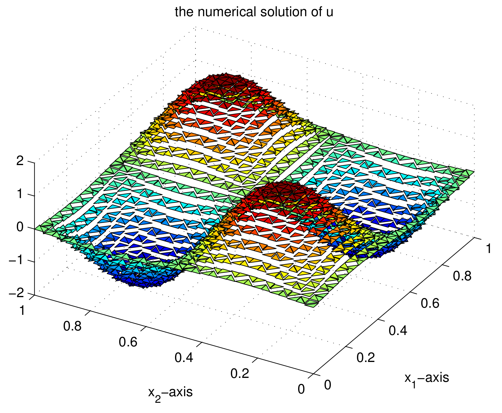
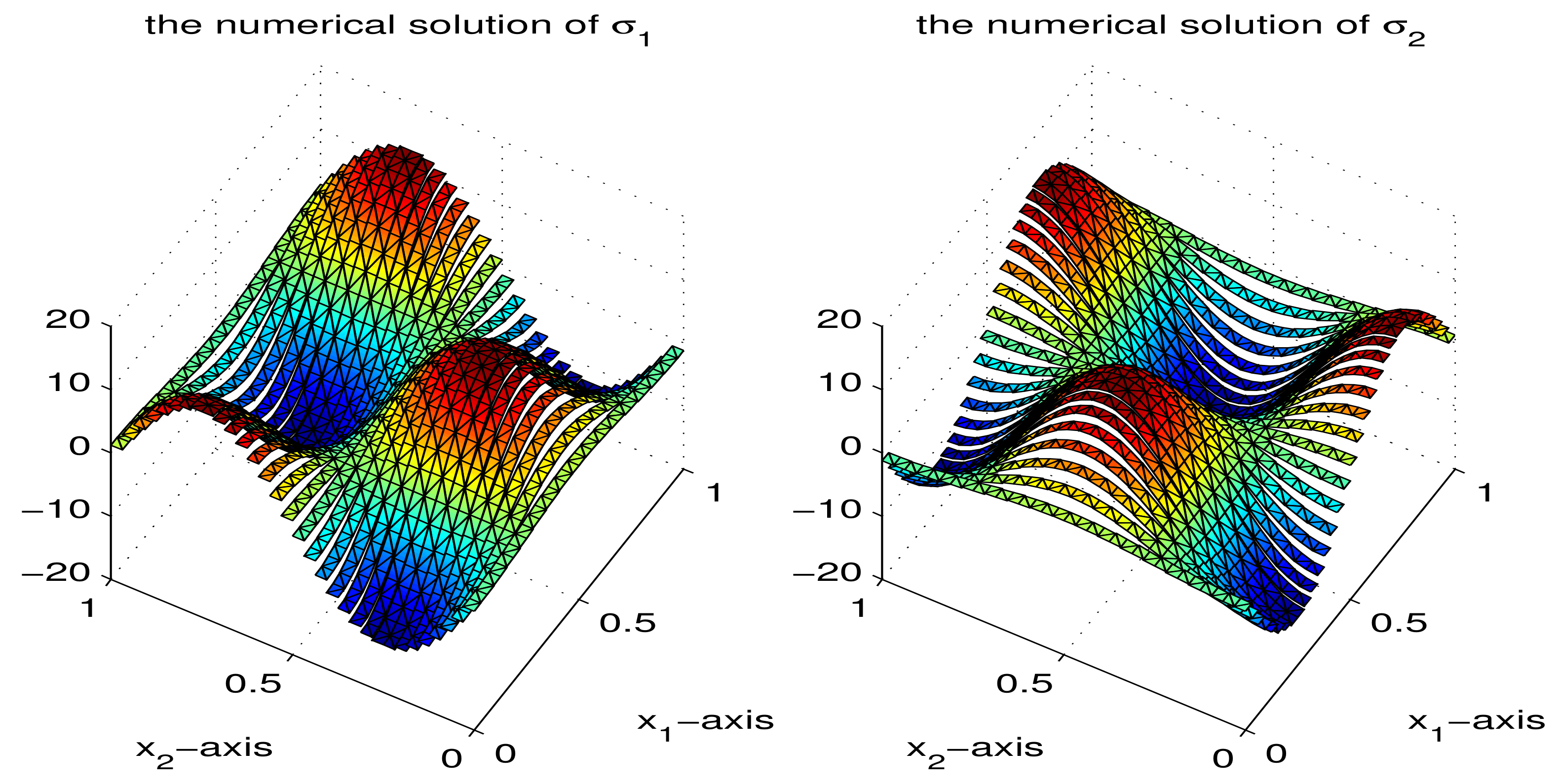
Example 2.

We consider the following time-fractional reaction-diffusion equation in two-dimensional spatial regions

$$\begin{array}{c}\hfill \left\{\begin{array}{cc}{\displaystyle \frac{{\partial }^{\alpha }u(X,t)}{\partial t^{\alpha }}}-\epsilon \Delta u(X,t)+p\left(X\right)u(X,t)=f(X,t),\hfill & (X,t)\in \Omega \times J,\hfill \\ u(X,t)=0,\hfill & (X,t)\in \partial \Omega \times \overline{J},\hfill \\ u(X,0)=sin\left(2\pi x_1\right)sin\left(2\pi x_2\right),\hfill & X=(x_1,x_2)\in \overline{\Omega },\hfill \end{array}\right.\end{array}$$

where $\Omega =(0,1)\times (0,1)$, $J=(0,1]$, $\epsilon =1$, $p\left(X\right)=1+x_1^2+x_2^2$, and the source function $f(X,t)=(\frac{2}{\Gamma (3-\alpha )}{t}^{2-\alpha }+8{\pi }^2(1+t^2)+(1+x_1^2+x_2^2)(1+t^2))sin\left(2\pi x_1\right)sin\left(2\pi x_2\right)$. Then, we can obtain the exact solutions

$$\begin{array}{c}u(X,t)=(1+t^2)sin\left(2\pi x_1\right)sin\left(2\pi x_2\right),\hfill \\ \mathbf{\sigma }(X,t)=(-2\pi (1+t^2)cos\left(2\pi x_1\right)sin\left(2\pi x_2\right),-2\pi (1+t^2)sin\left(2\pi x_1\right)cos\left(2\pi x_2\right)).\hfill \end{array}$$

In this example, we do some numerical experiments with different parameter $\alpha$ and mesh size $h=\sqrt{2}\tau$, and apply the fifth-order Gauss integral formula in triangular regions to calculate the errors of u (in $L^{\infty }\left(L^2(\Omega )\right)$-norm) and $\mathbf{\sigma }$ (in $L^{\infty }({\mathbf{L}}^2(\Omega )$-norm and $L^{\infty }\left(\mathit{H}(\mathrm{div},\Omega )\right)$-norm, where ${\mathbf{L}}^2(\Omega )={\left(L^2(\Omega )\right)}^2$). The numerical results show that the orders of convergence are approximate to 1. The numerical simulation results are given in

Table 7. Error results with $\alpha =0.1$ and $h=\sqrt{2}\tau$ for Example 2.

$\mathit{\tau },\mathit{h}$	${\parallel \mathit{u}-\mathit{U}\parallel }_{{\mathit{L}}^{\mathit{\infty }}\left({\mathit{L}}^2\right)}$	Order	${\parallel \mathit{\sigma }-\mathit{Z}\parallel }_{{\mathit{L}}^{\mathit{\infty }}\left({\mathit{L}}^2\right)}$	Order	${\parallel \mathit{\sigma }-\mathit{Z}\parallel }_{{\mathit{L}}^{\mathit{\infty }}\left(\mathit{H}\right(\mathrm{div}\left)\right)}$	Order
$1/10,\sqrt{2}/10$	$2.5821\times {10}^{-1}$		2.0257		$2.0380\times {10}^1$
$1/20,\sqrt{2}/20$	$1.3045\times {10}^{-1}$	0.9850	1.0089	1.0057	$1.0335\times {10}^1$	0.9796
$1/40,\sqrt{2}/40$	$6.5394\times {10}^{-2}$	0.9963	$5.0386\times {10}^{-1}$	1.0017	5.1860	0.9949
$1/80,\sqrt{2}/80$	$3.2718\times {10}^{-2}$	0.9991	$2.5185\times {10}^{-1}$	1.0004	2.5953	0.9987

with parameter $\alpha =0.1$ and mesh sizes $h=\sqrt{2}\tau =\frac{\sqrt{2}}{10},\frac{\sqrt{2}}{20},\frac{\sqrt{2}}{40},\frac{\sqrt{2}}{80}$, and the other results with different parameter $\alpha$ are similar. The graphs of numerical solutions for variables u and $\mathbf{\sigma }$ at time parameter $t=1$ with a space mesh size $h=\sqrt{2}\tau =\frac{\sqrt{2}}{40}$ are given in Figure 2 and Figure 3, respectively. Because the trial function spaces $L_h$ (defined in (6)) and ${\mathit{H}}_h$ (defined in (5)) are not continuous function spaces, the surfaces in Figure 2 and Figure 3 agree with the properties of the trial function spaces. The figures and numerical results show that the proposed MFVE method for the time-fractional reaction-diffusion equations in two-dimensional spatial regions is feasible and effective.

Remark 2.

When the diffusion coefficient ε in Examples 1 and 2 is chosen to be $1/100$, we do some numerical experiments with parameter $\alpha =0.1,0.3,0.5,0.7,0.9$. The numerical results show that the orders of convergence are similar to that of $\epsilon =1$. The numerical results with $\epsilon =1/100$ in Example 1 ($\alpha =0.1,0.3$) and Example 2 ($\alpha =0.1$) are given in

Table 8. Error results with $\alpha =0.1$ and h = 1$\times {10}^{-4}$ for Example 1 ($\epsilon =1/100$).

$\mathit{\tau }$	${\parallel \mathit{u}-\mathit{U}\parallel }_{{\mathit{L}}^{\mathit{\infty }}\left({\mathit{L}}^2\right)}$	Order	${\parallel \mathit{\sigma }-\mathit{Z}\parallel }_{{\mathit{L}}^{\mathit{\infty }}\left({\mathit{L}}^2\right)}$	Order	${\parallel \mathit{\sigma }-\mathit{Z}\parallel }_{{\mathit{L}}^{\mathit{\infty }}\left({\mathit{H}}^1\right)}$	Order
1/10	$3.2777\times {10}^{-4}$		$2.0606\times {10}^{-3}$		$1.3174\times {10}^{-2}$
1/20	$9.5057\times {10}^{-5}$	1.7858	$5.9811\times {10}^{-4}$	1.7846	$3.8224\times {10}^{-3}$	1.7852
1/40	$2.7240\times {10}^{-5}$	1.8031	$1.7192\times {10}^{-4}$	1.7987	$1.0971\times {10}^{-3}$	1.8008
1/80	$7.7041\times {10}^{-6}$	1.8220	$4.9147\times {10}^{-5}$	1.8066	$3.1205\times {10}^{-4}$	1.8139

,

Table 9. Error results with $\alpha =0.3$ and h = 1$\times {10}^{-4}$ for Example 1 ($\epsilon =1/100$).

$\mathit{\tau }$	${\parallel \mathit{u}-\mathit{U}\parallel }_{{\mathit{L}}^{\mathit{\infty }}\left({\mathit{L}}^2\right)}$	Order	${\parallel \mathit{\sigma }-\mathit{Z}\parallel }_{{\mathit{L}}^{\mathit{\infty }}\left({\mathit{L}}^2\right)}$	Order	${\parallel \mathit{\sigma }-\mathit{Z}\parallel }_{{\mathit{L}}^{\mathit{\infty }}\left({\mathit{H}}^1\right)}$	Order
1/10	$1.6068\times {10}^{-3}$		$1.0098\times {10}^{-2}$		$6.4601\times {10}^{-2}$
1/20	$5.1406\times {10}^{-4}$	1.6442	$3.2311\times {10}^{-3}$	1.6439	$2.0670\times {10}^{-2}$	1.6440
1/40	$1.6304\times {10}^{-4}$	1.6567	$1.0253\times {10}^{-3}$	1.6560	$6.5577\times {10}^{-3}$	1.6563
1/80	$5.1350\times {10}^{-5}$	1.6668	$3.2341\times {10}^{-4}$	1.6646	$2.0670\times {10}^{-3}$	1.6656

and

Table 10. Error results with $\alpha =0.1$ and $h=\sqrt{2}\tau$ for Example 2 ($\epsilon =1/100$).

$\mathit{\tau },\mathit{h}$	${\parallel \mathit{u}-\mathit{U}\parallel }_{{\mathit{L}}^{\mathit{\infty }}\left({\mathit{L}}^2\right)}$	Order	${\parallel \mathit{\sigma }-\mathit{Z}\parallel }_{{\mathit{L}}^{\mathit{\infty }}\left({\mathit{L}}^2\right)}$	Order	${\parallel \mathit{\sigma }-\mathit{Z}\parallel }_{{\mathit{L}}^{\mathit{\infty }}\left(\mathit{H}\left(\mathbf{div}\right)\right)}$	Order
$1/10,\sqrt{2}/10$	$2.5704\times {10}^{-1}$		2.0136		$2.0549\times {10}^1$
$1/20,\sqrt{2}/20$	$1.3029\times {10}^{-1}$	0.9803	1.0081	0.9982	$1.0348\times {10}^1$	0.9897
$1/40,\sqrt{2}/40$	$6.5373\times {10}^{-2}$	0.9949	$5.0378\times {10}^{-1}$	1.0007	5.1874	0.9963
$1/80,\sqrt{2}/80$	$3.2715\times {10}^{-2}$	0.9987	$2.5184\times {10}^{-1}$	1.0003	2.5955	0.9990

, the other results with different parameter α are not a repeat description.

7. Conclusions

We apply the MFVE method to treat the time-fractional reaction-diffusion equations. By introducing the auxiliary variable $\mathbf{\sigma }$ and applying the $L1$-formula, we construct the MFVE scheme, prove the existence and uniqueness of the proposed scheme, and obtain the stability results which only depend on the source term function $f(X,t)$. We also obtain a priori error estimates for the variable u (in $L^2(\Omega )$-norm) and the auxiliary variable $\mathbf{\sigma }$ (in ${\left(L^2(\Omega )\right)}^2$-norm and $\mathit{H}(\mathrm{div},\Omega )$-norm) by using generalized MFVE projection and the properties of the transfer operator ${\gamma }_h$. Moreover, we briefly describe that the MFVE method can also be constructed in one-dimensional spatial regions, and give two numerical examples to examine the feasibility and effectiveness. In this article, we consider a linear model. In the future, we will try to study some nonlinear fractional models by using our method, which will be a challenge for us from the point of view of numerical analysis.